DOA Estimation Using Triply Primed Arrays Based on
Fourth-Order Statistics
Kai-Chieh Hsu and Jean-Fu Kiang*
Abstract—A triply primed array (TPA) is configured on three mutually primed integers (N1,N2 and N3), which operates with O(N1N2N3) degree-of-freedoms to estimate the direction-of-arrivals (DOAs) of multiple incident quasi-stationary signals. The set of unique and contiguous lags of the proposed TPA is searched and verified. Simulation results verify that the proposed TPA can detect more incident signals with higher accuracy than its compatible counterparts.
1. INTRODUCTION
Direction-of-arrival (DOA) estimation is critical to radars and wireless communication systems. By processing the received signals from an N-element uniform linear array (ULA), subspace-based algorithms such as multiple signal classification (MUSIC) [1] and estimation of signal parameters via rotational invariance techniques (ESPRIT) [2] can be used to estimate at most N −1 sources. A Khatri-Rao (KR) subspace-based algorithm was proposed to increase the degrees-of-freedom (DOF) of an N-element ULA to 2N−2 [3].
Several array configurations with higher DOF have been proposed. In [4], a nested array was proposed to detect O(N2) sources with N sensors. However, the inter-element spacing is so small that mutual coupling effect becomes severe. In [5], a co-prime array was proposed, which is composed of two interleaved ULAs, one with M elements at N-interval spacing and the other with N elements at M-interval spacing, where M and N are mutually primed integers. The number of elements in one constituent array was increased from M to 2M, extending the range of contiguous virtual lags to
−M N ∼ M N [6]. By applying MUSIC algorithm, with the covariance matrix processed by a spatial smoothing technique, the DOF reachesO(M N). In [7], a MUSIC-based method with array interpolation and matrix denoising was proposed to fill the holes in a virtual coarray and reduce the estimation error of covariance matrix due to finite snapshots. In [8], an ESPRIT-based method was proposed to estimate the DOAs without resorting to spatial smoothing, peak search or a predefined grid.
Sparse signal processing techniques, such as compressive sensing (CS), have been used for DOA estimation. In [9], a CS-MUSIC algorithm was proposed on the relation between multiple measurement vectors and the estimated DOAs. In [10], an 1-optimization was proposed for sparse signal recovery, where1norm was imposed to ensure sparsity. In [11], co-prime arrays were generalized to include nested array [4] as a special case. In [12], a nearest grid DOA estimation method, supported by Rife algorithm, was proposed to detect DOAs that were off the grid. In [13], a low-complexity 1-normalization was proposed to merge same or conjugated lags. In general, the CS methods render higher DOF than MUSIC and perform better than the latter. However, the CS methods have difficulties in estimating off-grid DOAs and take heavier computational load.
In the aforementioned algorithms, received signals up to the second-order statistics were used. The performance is expected to improve if higher-order statistics can be used. In [14], MUSIC algorithm
Received 24 January 2018, Accepted 24 March 2018, Scheduled 5 April 2018
* Corresponding author: Jean-Fu Kiang ([email protected]).
was applied to process fourth-order cumulant matrix to mitigate mutual coupling effects. In [15], 1-normalization was applied to a fourth-order difference matrix to increase the range of contiguous lags. In this work, we propose a triply primed array (TPA), which is composed of three arrays specified by three mutually primed integers. By processing fourth-order statistics, higher DOF can be acquired by increasing the numbers of lags and contiguous lags. This paper is organized as follows. The signal model is presented in Section 2, the properties of TPA are analyzed in Section 3, the DOA estimation algorithms and dimension-reduction approach are presented in Section 4, and the simulation results are discussed in Section 5. Finally, some conclusions are drawn in Section 6.
2. SIGNAL MODEL OF TRIPY PRIMED ARRAY
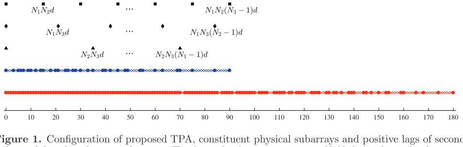
Figure 1 shows the proposed TPA, which is composed of three ULAs, with N1, N2 and N3 sensors, respectively; where N1, N2 and N3 are mutually primed integers. Without loss of generality, assume N1 < N2 < N3 and the unit spacing is d=λ/2. The spacings in the first, second and third ULAs are N2N3d,N1N3dand N1N2d, respectively. The first sensors of the three ULAs are aligned at the origin, leading to a total of N =N1+N2+N3−2 sensors in the TPA. The locations of the physical sensors in these three ULAs are specified in Γ1, Γ2 and Γ3, respectively, with
Γ1={n1N2N3d|0≤n1 ≤N1−1}, Γ2={n2N1N3d|0≤n2 ≤N2−1}, Γ3={n3N1N2d|0≤n3 ≤N3−1}
(1)
Assume that there are M uncorrelated source signals. The DOA of the mth source signal sm is
θm, with 1≤m≤M. The signals received at theth time interval can be represented as
¯
x1[] = ¯A1¯ ·¯s[] + ¯n1[], x2¯ [] = ¯A2¯ ·s¯[] + ¯n2[], x3¯ [] = ¯A3¯ ·¯s[] + ¯n3[] (2)
where ¯s[] is the source signal vector, and ¯A¯α and ¯nα are the steering matrix and noise vector,
respectively, of the αth ULA, withα = 1,2,3. Themth column of each steering matrix is the steering vector associated with themth source signal. Explicitly,
¯
a1(θm) =
1, ejkN2N3dsinθm, . . . , ejkN2N3(N1−1)dsinθm
t
,
¯
a2(θm) =
1, ejkN1N3dsinθm, . . . , ejkN1N3(N2−1)dsinθm
t
,
¯
a3(θm) =
1, ejkN1N2dsinθm
, . . . , ejkN1N2(N3−1)dsinθmt
where k = 2π/λ is the wavenumber. The additive white Gaussian noise vectors ¯n1[], ¯n2[] and ¯n3[] have zero mean and covariance matrices σn2I¯¯N1, σn2I¯¯N2 and σn2I¯¯N3 respectively, where ¯I¯N is an N ×N
0 10 20 30 40 50 60 70 80 90 100 110 120 130 140 150 160 170 180
identity matrix. Each noise vector is assumed to be uncorrelated to the source signals and the other noise vectors. The received signals in (2) are concatenated as
¯
x[] = ¯A¯·s¯[] + ¯n[] (3) where
¯ x[] =
⎡ ⎢ ⎢ ⎢ ⎣ ¯ x1[]
¯ x2[]
¯ x3[]
⎤ ⎥ ⎥ ⎥
⎦, A¯¯= ⎡ ⎢ ⎢ ⎢ ⎢ ⎣ ¯ ¯ A1 ¯ ¯ A2 ¯ ¯ A3 ⎤ ⎥ ⎥ ⎥ ⎥
⎦, n¯[] = ⎡ ⎢ ⎢ ⎢ ⎣ ¯ n1[]
¯ n2[]
¯ n3[]
⎤ ⎥ ⎥ ⎥ ⎦
Assume that the source signals are wide-sense quasi-stationary and are measured over Q non-overlapped time frames, with each time frame containing Ltime intervals [3, 13]. The power of themth source signal in the qth time frame can be represented as
Pqm = E
|sm[]|2
, 1≤q≤Q,(q−1)L≤≤qL−1 (4)
wherePqm with 1≤q≤Q are wide-sense stationary and uncorrelated from each other, namely,
Eq{Pqm}=μm, Eq
(Pqm−μm)2
= ˜σ2m (5)
The covariance matrix of the received signals in theqth time frame can be represented as ¯
¯
Rxxq = E{x¯q[]¯xq†[]}= ¯A¯·D¯¯xxq·A¯¯†+σ2nI¯¯N (6)
where ¯xq[] is the received signal at theqth time frame and ¯D¯xxq = diag{Pq1, Pq2, . . . , PqM}. In practice,
¯ ¯
Rxxq is estimated as
˜ ¯ ¯ Rxxq =
1 L
qL−1
=(q−1)L
¯
xq[]¯xq†[] (7)
All the columns of ¯R¯xxq are concatenated into an N2×1 vector as
¯
yq = vec
¯ ¯ Rxxq
= ¯B¯·P¯q+σn2ν¯N (8)
where ¯Pq = [Pq1, Pq2, . . . , PqM]t, ¯νN = vec{I¯¯N}, and ¯B¯ = ¯A¯∗A¯¯is the second-order difference manifold
matrix, withthe column-wise Kronecker product.
To obtain the fourth-order difference coarray, first take the expectation value of ¯yq to have
¯
yq = E{y¯q}= ¯B¯·P¯q+σn2ν¯N (9)
where ¯Pq = Eq
¯
Pq
= [μ1, μ2, . . . , μM]t Next, subtract (9) from (8) to obtain
¯
yq= ¯yq−y¯q = ¯B¯·
¯
Pq−P¯q
= ¯B¯·P¯q (10)
Thus,Qsignals are derived from the second-order statistics of the original received signals. Similar to (6) and (7), derive the covariance matrix of ¯yq and its estimation as
¯ ¯
Ryy= E{y¯qy¯q†}= ¯B¯·D¯¯yy·B¯¯† (11)
˜ ¯ ¯ Ryy=
1 Q Q q=1 ¯
yqy¯q† (12)
where ¯D¯yy = diag
˜
σ21,σ˜22, . . . ,σ˜M2
. By vectorizing ¯R¯yy, we obtain
¯ z= vec
¯ ¯ Ryy
= ¯C¯·ψ¯ (13)
where ¯ψ=σ˜2
1,σ˜22, . . . ,σ˜M2
t
3. PROPERTIES OF TRIPLY PRIMED ARRAY
3.1. Second-Order Virtual Array
Define self-difference matrices and cross-difference matrices between these three constituent subarrays as
¯ ¯
Rααq = E{x¯qα[]¯xqα†[]}= ¯A¯α·D¯¯xxq·A¯¯†α+σα2I¯¯Nα ¯
¯
Rαβq = E{x¯qα[]¯x q†
β []}= ¯A¯α·D¯¯xxq·A¯¯†β +σ
2
βW¯¯αβ (14)
where 1 ≤α, β ≤3, ¯W¯αβ is an Nα×Nβ matrix with the 00th entry equal to 1 and the other entries
equal to zero. The uvth entry of ¯R12¯ q is
R12q[u, v] =
⎧ ⎪ ⎪ ⎪ ⎪ ⎪ ⎪ ⎪ ⎪ ⎪ ⎪ ⎨ ⎪ ⎪ ⎪ ⎪ ⎪ ⎪ ⎪ ⎪ ⎪ ⎪ ⎩
M
m=1
PqmejkN3(uN2−vN1)dsinθm+σn2,
u=v= 0
M
m=1
PqmejkN3(uN2−vN1)dsinθm,
u= 0 or v= 0
(15)
It is observed that R12q[u, v] andR12q[N1−u, N2 −v] are conjugate to each other with u, v = 0. In
addition, the lags of entries in the first column of ¯R21¯ q overlap with those of some diagonal entries of
¯ ¯
R11q, and the lags of entries in the first row of ¯R21¯ q overlap with those in some diagonal entries of ¯R22¯ q,
which implies that ¯R21¯ q is redundant in counting the number of unique lags. As a result, only ¯R12¯ q,
¯ ¯
R23q and ¯R31¯ q are needed. Thus, all the unique lags of a second-order virtual array are included in the
union of Γ0 ={0} and six disjoint sets,
Γ12={N3(n1N2−n2N1)d|1≤n1≤N1−1,1≤n2 ≤N2−1}, Γ23={N1(n2N3−n3N2)d|1≤n2≤N2−1,1≤n3 ≤N3−1}, Γ31={N2(n3N1−n1N3)d|1≤n1≤N1−1,1≤n3 ≤N3−1},
Γ11={n1N2N3d|1≤ |n1| ≤N1−1}, Γ22={n2N1N3d| 1≤ |n2| ≤N2−1}, Γ33={n3N1N2d|1≤ |n3| ≤N3−1},
(16)
where Γαβ ={p−q |p∈Γα, q∈Γβ, p, q= 0}.
3.2. Fourth-Order Virtual Array
Based on the six sets in Eq. (16), 36 fourth-order difference sets can be derived. Since all the second-order difference sets are symmetric, the derived fourth-second-order difference sets are also symmetric, and Γαβ,αβ = Γαβ,αβ.
The difference lags between Γ11, Γ22, Γ33 and Γ12 are listed below.
Γ11,11={n1N2N3d|1≤ |n1| ≤2N1−2}, Γ22,22={n2N1N3d|1≤ |n2| ≤2N2−2}, Γ33,33={n3N1N2d|1≤ |n3| ≤2N3−2},
Γ12,12={N3(n1N2−n2N1)d|2−N1 ≤n1 ≤N1−2,2−N2 ≤n2≤N2−2}, Γ12,11={N3(n1N2−n2N1)d|2−N1 ≤n1 ≤2N1−2,1≤n2≤N2−1}, Γ12,22={N3(n1N2−n2N1)d|1≤n1≤N1−1,2−N2≤n2 ≤2N2−2},
Γ12,33={(n1N2N3−n2N1N3−n3N1N2)d|1≤n1 ≤N1−1,1≤n2 ≤N2−1,1≤ |n3| ≤N3−1}, Γ11,22={N3(n1N2−n2N1)d|1≤ |n1| ≤N1−1,1≤ |n2| ≤N2−1},
Γ22,33={N1(n2N3−n3N2)d|1≤ |n2| ≤N2−1,1≤ |n3| ≤N3−1}, Γ33,11={N2(n3N1−n1N3)d|1≤ |n1| ≤N1−1,1≤ |n3| ≤N3−1},
It is observed that Γ12,12⊆Γ11,22.
Letμ=N3(n1N2−n2N1)d∈Γ12,11,ν =N3(n1N2−n2N1)d∈Γ11,22 and ξ =n2N1N3d∈Γ22,22. It is observed that
⎧ ⎨ ⎩
μ=ν, (n1, n2) = (n1, n2), 2−N1 ≤n1 ≤N1−1
μ=ν, (n1, n2) = (n1−N1, n2−N2), N1+ 1≤n1≤2N1−2 μ=ξ, n2 =N2−n2, n1=N1
(18)
which implies that Γ12,11 ⊆ (Γ11,22∪Γ22,22). Similarly, Γ12,22 is included in the union of some other sets. As a result, the remaining 7 sets in Eq. (17) are disjoint to one another.
Next, letμ= (n2N1N3−n3N1N2−n1N2N3)d∈Γ23,11 andν = (n1N2N3−n2N1N3−n3N1N2)d∈ Γ12,33. It is observed that
(n1, n2, n3) =
(N1−n1, N2−n2, n3), n1 ≤0
(−n1, N2−n2,−N3+n3), n1 >0 (19)
which implies that Γ23,11 = Γ12,33. Let μ = (n1N2N3 − n2N1N3 + n3N1N2)d ∈ Γ12,23, ν =
(n1N2N3 −n2N1N3 −n3N1N2)d ∈ Γ12,33 and ξ = (n3N1N2 −n1N2N3)d ∈ Γ33,11. It is observed
that
⎧ ⎨ ⎩
μ=ν, (n1, n2, n3) = (n1, n2,−n3), 2≤n2 ≤N2−1
μ=ν, (n1, n2, n3) = (n1, n2−N2,−n3+N3), N2+ 1≤n2 ≤2N2−2 μ=ξ, (n1, n3) = (−n1, n3−N3), n2=N2
(20)
which implies that the lags in Γ12,23 are included in Γ12,33 or Γ33,11. From Eqs. (18)–(20), all the fourth-order difference lags are included in 8 disjoint sets, Γ11,11, Γ22,22, Γ33,33, Γ11,22, Γ22,33, Γ33,11, Γ12,33and Γ0. The number of unique fourth-order difference lags will be equal to the sum of cardinality of these 8 sets.
It is observed that the lags in Γ11,11, Γ22,22, Γ33,33 and Γ12,33 are mutually disjoint. On the other hand, some lags in Γ11,22, Γ22,33 and Γ33,11 are overlapped. Consider μ=N3(n1N2−n2N1)d∈Γ11,22 and ν = N3(n1N2−n2N1)d∈Γ11,22, μ =ν only when (n1, n2) = (n1−N1, n2 −N2) and n1, n2 > 0, leading to 2(N1−1)2(N2−1)−(N1−1)(N2−1) = 3(N1−1)(N2−1) unique lags in Γ11,22. As a result,
the number of unique lags in the fourth-order difference set is
τu = (4N1−4) + (4N2−4) + (4N3−4) + 3(N1−1)(N2−1) + 3(N2−1)(N3−1)
+3(N1−1)(N3−1) + 2(N1−1)(N2−1)(N3−1) + 1
= 2N1N2N3+N1N2+N2N3+N3N1−8 (21)
It is also observed that the contiguous lags in the fourth-order difference set fall in the range [−τc, τc],
with τc =N1N2+N2N3+N3N1−1. Note that lag at N1N2+N2N3+N3N1 does not belong to any
of the 8 sets defined in Section III-B.
4. DOA ESTIMATION ALGORITHMS
Conventional subspace-based algorithms like MUSIC and ESPRIT require the rank of covariance matrix be higher than the number of source signals. As shown in Eq. (13), ¯ψ is a vector, and the covariance matrix ¯R¯zz = ¯zz¯† is of rank one. A spatial-smoothing MUSIC (SS-MUSIC) algorithm can be applied
to a virtual array based on ¯z, with rank significantly higher than one. A CS approach can be applied to solve an 1 optimization problem instead, with no restriction to the rank. These two methods are briefly reviewed in this Section.
4.1. Spatial-smoothing MUSIC Algorithm
The SS-MUSIC algorithm was proposed to increase the rank [6], but it can only be applied to virtual arrays with contiguous lags. To apply SS-MUSIC, non-contiguous lags of ¯z are first removed to form
¯
where ¯C¯c is constructed on a ULA with 2τc+ 1 sensors located from−τcdtoτcd. Next, constructτc+ 1
sub-vectors, each withτc+ 1 elements, as
¯
zcξ = [zc[ξ−τc], zc[ξ−τc+ 1], . . . , zc[ξ−1], zc[ξ]]t, 0≤ξ ≤τc (23)
Then derive a matrix
¯ ¯ Rzz,ss=
1 τc+ 1
τc
ξ=0 ¯
zcξz¯cξ† (24)
of which the rank is τc+ 1. The MUSIC algorithm is then applied to ¯R¯zz,ss to estimate the DOAs.
4.2. Compressive Sensing Algorithm
Before applying the CS approach, first formulate a sensing matrix ¯C¯g composed of G steering vectors
as
¯ ¯
Cg= [¯cg(φ1),c¯g(φ2), . . . ,c¯g(φG)] (25)
where
¯
cg(φα) = [¯a∗(φα)⊗¯a(φα)]⊗[¯a∗(φα)⊗a¯(φα)]
φα=−90◦+ 180◦(α−1)/(G−1), 1≤α≤G
and⊗stands for Kronecker product. Then, Eq. (13) is transformed to an1-norm minimization problem ¯
ψ◦g = arg min
¯
ψg
ψ¯g1 s.t. z¯−C¯¯g·ψ¯g2< (26)
whereis a given error bound, and · p means thep norm. Eq. (26) can be solved by using a software
package CVX [16, 17]. The indices of nonzero entries in ¯ψg◦ are mapped to the estimated DOAs.
4.3. Dimension-Reduced Algorithm
The dimension of ¯C¯ in Eq. (13) is N4 ×G, making the computational load impractical for real-time applications. In this Subsection, a modified version of dimension-reduced approach [13] for coprime arrays is proposed to support the TPA.
The expression in Eq. (15) indicates that some entries of ¯yq in Eq. (8) have the same lag or
conjugated lag, which can be merged to reduce the dimension and increase the accuracy of DOA estimation. Entries with the same lags should have the same value in principle, but they are different in practice due to noise or other errors. Taking the average of different entries associated with a lag results in better accuracy of DOA estimation. To begin with, construct a vector
¯
yααq = [rααq∗ [Nα−1], . . . , rααq∗ [1], rααq[1], . . . , rααq[Nα−1]]t, α= 1,2,3
with
rααq[n] =
1 2(Nα−n)
Nα−1−n
n=0
Rααq[n+n, n] +R∗ααq[n, n+n]
(27)
Then, vectorize ¯R¯12q to obtain ¯y12q, with the uvth entry of ¯R¯12 q defined as
R12q[u, v] =R12q[u+ 1, v+ 1] +R∗12q[N1−1−u, N2−v−1] (28)
Similarly, ¯y23q and ¯y31q are obtained by vectorizing ¯R¯23q and ¯R¯31 q, respectively.
Next, form a dimension-reduced vector ¯yqr as
¯
yqr= [y0q,y¯t11q,y¯22t q,y¯33t q,y¯12t q,y¯23t q,y¯t31q]t= ¯BΦB¯ ·P¯¯q+σn2w,¯ (29)
where
y0q=
1 N
N 1−1
n=0
R11q[n, n] + N2−1
n=1
R22q[n, n] + N3−1
n=1
R33q[n, n]
1000 2000 3000 4000 5000 6000 7000 8000 9000 10000 -5
0 5
1000 2000 3000 4000 5000 6000 7000 8000 9000 10000 -5
0 5
Figure 2. Simulated quasi-stationary signals (——), time frames are bounded by. . ..
¯ ¯
BΦB is a sub-matrix constituted of rows in ¯B¯ which are indexed by ΦB. Each element of ΦB indicates
a unique lag, and ¯wis a vector with first entry equal to one and the others equal to zero. By applying the procedure in Eqs. (8)–(12) to ¯yqr, we have
¯
yqr = ¯yqr−E{y¯qr}= ¯BΦB¯ ·P¯¯q
¯ ¯
Ryyr = E{y¯qry¯†qr}= ¯BΦB¯ ·D¯¯yy·B¯¯ΦB† ˜ ¯ ¯ Ryyr =
1 Q
Q
q=1 ¯
yqry¯†qr (31)
Then, Eq. (13) is modified as
¯ z = vec
¯ ¯ Ryyr
= ¯C¯·ψ¯ (32)
where ¯C¯ = ¯B¯ΦB∗ BΦB¯¯ .
By imposing Eqs. (18)–(20), entries of ¯z with the same or conjugated lag are merged. A dictionary is prepared to record the corresponding lag of each entry in ¯z. By using this dictionary, a dimension-reduced ¯zr is derived as
¯
zr = ¯zΦC = ¯C¯ΦC ·ψ¯ (33) where ΦC is the set of indices corresponding to all the positive lags in the fourth-order difference set,
and |ΦC|= (τu+ 1)/2. Finally, Eq. (26) is reformed as
¯
ψg◦ = arg min
¯
ψg
ψ¯g1 s.t. z¯r−C¯¯
g,ΦC ·ψ¯g2 < , (34)
where ¯C¯g = ¯B¯g,∗ΦB B¯¯g,∗ΦB.
5. SIMULATIONS AND DISCUSSIONS
In this work, TPA(3, 4, 5) and TPA(3, 5, 7) are constructed and compared with CPA(3, 5). TPA(3, 4, 5) and CPA(3, 5) are composed of 10 physical sensors, while TPA(3, 5, 7) is composed of 13 physical sensors. The unit spacing is d = λ/2 in all the three arrays. Without loss of generality, the DOAs of M signal sources are uniformly distributed over [−60,60◦]. Fig. 2 shows two sample segments of quasi-stationary source signals, with stationary intervals randomly chosen from a uniform distribution between [300, 700] samples [3]. The noise is specified in terms of the signal-to-noise ratio (SNR), which is defined as
SNR = 1 T
T
=1 E
A¯¯·¯s[]2
E
n¯[]2
-60 -50 -40 -30 -20 -10 0 10 20 30 40 50 60 0
0.2 0.4 0.6 0.8 1
-60 -50 -40 -30 -20 -10 0 10 20 30 40 50 60 0
0.2 0.4 0.6 0.8 1
(b) (a)
Figure 3. Normalized spectrum of (a) TPA (3, 4, 5) and (b) CPA (3, 5); M = 61, SNR = 5 dB, L = 500, Q = 1,000. ———: estimated power spectrum; ——: actual power spectrum; ——: actual DOAs.
where T =LQ [3]. The grid spacing of sensing matrix is 0.05◦, and is chosen by trial-and-error. In each scenario, 100 Monte-Carlo realizations are simulated.
Figure 3 shows the normalized spectrum of TPA (3, 4, 5) and CPA (3, 5), respectively, where the actual power spectrum is ¯ψ in Eq. (13), and the estimated power spectrum is ¯ψg◦ in Eq. (34). The
spectrum is normalized with respect to the largest entry in the original spectrum. The length of each time frame is fixed at L in the estimation algorithms. In Eq. (34), the vector length, z¯r2, of TPA(3, 4, 5) and CPA(3, 5) is about 6, and the error bound is empirically chosen as = 1. It is observed that all the signal sources are accurately detected by the TPA, but the CPA misses some signal sources and mistakenly detects non-existing signal sources between actual DOAs.
To compare the performance of different methods, a root-mean-square-error (RMSE) of DOA estimation is defined as
RMSE =
1
KM
K
k=1
M
m=1
|θ˜km−θm|2, (36)
where θm and ˜θkm are the actual DOA and the estimated DOA, respectively, of the mth source signal
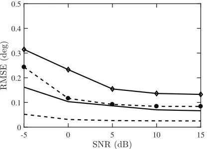
-5 0 5 10 15 0
0.1 0.2 0.3 0.4 0.5
Figure 4. RMSE of DOA estimations under different SNRs; M = 36, L = 500, Q = 1,000. ——: TPA (3, 4, 5), CS;− • −: TPA(3, 4, 5), SS-MUSIC;− −: CPA(3, 5), CS;− − −: TPA(3, 5, 7), CS.
200 400 600 800 1000 0
0.2 0.4 0.6 0.8 1 1.2 1.4
Figure 5. RMSE of DOA estimations with different numbers of frames; M = 36, L = 500, SNR = 0 dB. ——: TPA (3, 4, 5), CS; − • −: TPA (3, 4, 5), SS-MUSIC;− −: CPA (3, 5), CS;
in the kth realization. Fig. 4 shows the RMSE of DOA estimation under different SNRs by using CS approach on TPA and CPA, as well as SS-MUSIC on TPA. In this case, the optimum values of for TPA (3, 4, 5), TPA(3, 5, 7) and CPA, under SNR = [−5,0,5,10,15] dB, are [4.3,2,1.5,1,1], [4,1,0.8,0.8,0.8] and [4,1,0.7,0.6,0.5], respectively. It is observed that the estimation results are less sensitive to the value ofwhen SNR is greater than 0 dB. A larger is suggested when SNR is less than 0 dB. Fig. 4 shows the TPA supported by either SS-MUSIC or CS approach predicts accurate DOAs under all SNRs, especially when SNR<0 dB. The CS approach predicts more accurate DOAs than the SS-MUSIC because the former makes use of all the unique lags, while the latter uses only contiguous lags.
Figure 5 shows the RMSE of DOA estimation with different numbers of frames. In this case, the optimum values of for TPA(3, 4, 5), TPA(3, 5, 7) and CPA, with Q = [200,400,600,800,1000], are [3.5,3,2,2,2], [2,2,2,2,1] and [1.5,1,1,1,1], respectively. The accuracy of DOA estimation is insensitive to when the latter is not far from the optimum value. The TPA supported by CS approach gives more accurate estimation than the other two, and the accuracy degrades smoothly when the number of frames decreases. The SS-MUSIC algorithm is more sensitive to the accuracy ofR˜¯¯yy in Eq. (12), as
compared to the CS approach.
200 300 400 500 600 700 0
0.1 0.2 0.3 0.4 0.5
Figure 6. RMSE of DOA estimations with different lengths of frame; M = 36, Q = 1,000, SNR = 0 dB. ——: TPA (3, 4, 5), CS; − • −: TPA (3, 4, 5), SS-MUSIC; − −: CPA (3, 5), CS; − − −: TPA (3 5, 7), CS.
Figure 6 shows the RMSE of DOA estimation with different lengths of frame. In this case, the optimum values of for TPA(3, 4, 5), TPA(3, 5, 7) and CPA, with L = [200,300,400,500,600,700], are [3,2.5,2.5,2,2,2], [3,2,1.5,1.2,1,1] and [2.5,2,1,1,1,1], respectively. Similar to the previous cases, the accuracy of DOA estimation is insensitive to if the latter is not far from the optimum value. It is observed that TPA supported by CS approach is hardly affected by the change ofLdue to the increased number of DOFs. The RMSE of CPA supported by CS approach and TPA supported by SS-MUSIC algorithm increases whenLdeviates from 500, possibly related to the estimation of power in each time frame.
6. CONCLUSION
A triply primed array (TPA) based on three mutually prime numbers (N1,N2 and N3) is proposed to achieve O(N1N2N3) DOFs in the fourth-order covariance matrices by exploiting the quasi-stationary signals. The properties of the proposed TPA are analyzed, and both SS-MUSIC algorithm and CS approach are applied to estimate the DOAs of signal sources. Simulation results show that the TPA can detect more signal sources with higher resolution than conventional CPA due to higher DOF of the former.
REFERENCES
1. Schmidt, R., “Multiple emitter location and signal parameter estimation,” IEEE Trans. Antennas Propagat., Vol. 34, No. 3, 276–280, 1986.
2. Roy, R. and T. Kailath, “ESPRIT-estimation of signal parameters via rotational invariance techniques,” IEEE Trans. Acous. Speech Signal Process., Vol. 37, No. 7, 984–995, 1989.
3. Mao, W. K., T. H. Hsieh, and C. Y. Chi, “DOA estimation of quasi-stationary signals with less sensors than sources and unknown spatial noise covariance: A Khatri-Rao subspace approach,”
IEEE Trans. Signal Process., Vol. 58, No. 4, 2168–2180, 2010.
4. Pal, P. and P. P. Vaidyanathan, “Nested arrays: A novel approach to array processing with enhanced degrees of freedom,” IEEE Trans. Signal Process., Vol. 58, No. 8, 4167–4181, 2010. 5. Vaidyanathan, P. P. and P. Pal, “Sparse sensing with co-prime samplers and arrays,” IEEE Trans.
Signal Process., Vol. 59, No. 2, 573–586, 2011.
6. Pal, P. and P. P. Vaidyanathan, “Coprime sampling and the MUSIC algorithm,” Proc. IEEE
DSP/SPE Workshop, 289–294, 2011.
7. Guo, M., T. Chen, and B. Wang, “An improved DOA estimation approach using coarray interpolation and matrix denoising,”Sensors, Vol. 17, No. 5, 1140, 2017.
8. Zhou, C. and J. Zhou, “Direction-of-arrival estimation with coarray ESPRIT for coprime array,”
Sensors, Vol. 17, No. 8, 1779, 2017.
9. Kim, J. M., O. K. Lee, and J. C. Ye, “Compressive MUSIC: Revisiting the link between compressive sensing and array signal processing,”IEEE Trans. Info. Theory, Vol. 58, No. 1, 278–301, 2012. 10. Zhang, Y. D., M. G. Amin, and B. Himed, “Sparsity-based DOA estimation using co-prime arrays,”
IEEE Int. Conf. Acous. Speech Signal Process., 3967–3971, 2013.
11. Qin, S., Y. D. Zhang, and M. G. Amin, “Generalized coprime array configurations for direction-of-arrival estimation,” IEEE Trans. Signal Process., Vol. 63, No. 6, 1377–1390, 2015.
12. Xu, L., J. Chen, and Y. Gao, “Off-grid DOA estimation based on sparse representation and rife algorithm,”Prog. Electromag. Res. M, Vol. 59, 193–201, 2017.
13. Shen, Q., W. Liu, W. Cui, S. Wu, Y. D. Zhang, and M. G. Amin, “Low-complexity direction-of-arrival estimation based on wideband co-prime arrays,” IEEE/ACM Trans. Audio Speech Lang. Process., Vol. 23, No. 9, 1445–1456, 2015.
14. Liu, S., J. Zhao, and Z. Xiao, “DOA estimation with sparse array under unknown mutual coupling,”
Prog. Electromag. Res. Lett., Vol. 70, 147–153, 2017.
15. Shen, Q., W. Liu, W. Cui, and S. Wu, “Extension of co-prime arrays based on the fourth-order difference co-array concept,” IEEE Signal Process. Lett., Vol. 23, No. 5, 615–619, 2016.
16. CVX Research Inc., “CVX: Matlab Software for Disciplined Convex Programming, version 2.0 beta,”http://cvxr.com/cvx, 2013.