A Novel of Surface Reflection Method Using Radio-Wave
for Soil Density Estimation
Roslee Mardeni*, Intan S. Shahdan, and Khazaimatol S. Subari
Abstract—Soil density is one of the important parameters to be investigated in civil, geological and agricultural works. Unfortunately, the challenging issue is found on a suitable model in determining accurately the soil density. In this article, a new soil density model based on radio-wave surface reflection method is presented. The development of the model is based on result analysis collected from the experiment. Then, comparisons with related theoretical models, Hallikainen and Topp, are performed. The experiment is performed by using a vector network analyzer (VNA) that generates radar signal and recording return loss (S11) from a horn antenna. In the analysis, two new proposed soil density
models have shown good agreement for soil density from 1.1 g/cm3 to 1.7 g/cm3 for sand and silty sand samples. This is verified when the model able to predict real samples as the one used in the experiment and result shows a very small relative error within 0.05% and 6.87%. Additionally, spectrograms in real time are produced in this study in order to observe more on the soil density. By using the proposed developed models, soil density estimation can be easily determined with minimal data input such as soil type, return loss and reflection coefficient by using regular radio-wave devices.
1. INTRODUCTION
In civil, geological and agricultural works, soil density is one of the important parameters to be investigated [1]. Over the years, many researchers concentrate on geophysical surveys where they need to study and evaluate geological structure non-destructively [2–4]. Geophysical or remote-sensing method is more preferable in recent years. It is able to measure and predict structure condition and parameters such as soil moisture, mineral content, buried target in the ground, cracks in concrete, and pipe leakage in the wall [3, 4]. Besides, reflected wave signals have been explored on other materials such as road pavement and hot-mix asphalt (HMA) using dielectric mixing models [5]. Unfortunately those methods are found complex, expensive and destructive.
In this article, we propose an alternative method without having to make major disturbances to the structure, which has been proven to be quite accurate, much faster and in most cases, much cheaper than the conventional methods. Our proposed soil density model is expected to give a faster density estimation that can benefit agricultural surveyors’ doing their routine soil density test. The models are developed from result analysis produced by conducting radio-wave reflection measurements at microwave frequency from 1.7 GHz to 2.7 GHz. The novelty of the proposed soil density model is that there is no any existing model in terms of soil density specifically. The existing models that have been used are in terms of soil moisture content and require unknown parameters that are not easily accessible by many engineers. In our new proposed soil density models, the input parameters needed are only soil type and return loss values, which can be obtained by simple microwave measurement devices.
Received 18 May 2014, Accepted 29 July 2014, Scheduled 17 August 2014
* Corresponding author: Roslee Mardeni ([email protected]).
permeability and conductivity [6, 7]. Moisture content is one of the popular parameters to be investigated according to [8–10]. This is because the moisture content information is very important in many areas especially in agricultural and civil engineering according to [11]. In relation with density, in this study, moisture content was varied from 0% to 20% for four soil samples of different types from sand to clay. The experiments were done in the laboratory where the samples were placed in a coaxial transmission line, and the complex dielectric permittivity was measured from dry soil up to saturated condition. An empirical model of soil moisture content in terms of dielectric permittivity was introduced and expressed as below:
mv =−5.3×10⁻²+2.92×10⁻²ε−5.5×10⁻⁴ε2+4.3×10⁻⁶ε3 (1)
wheremv is the volumetric soil moisture content in cm3/cm3, andεis the real part of complex relative permittivity of the soil. In a case where soil moisture content is known, the dielectric permittivity of the soil can be obtained by rearranging Equation (1) as:
ε= 3.03 + 9.3mv+ 146.0m2v+ 76.7m3v (2) In the study, soil types have shown dielectric permittivity changes significantly in the lower frequency range particularly between 1.4 GHz to 5 GHz. The improved models by [12] up to 2nd degree polynomial at 1.4 GHz are shown below:
ε=(2.862−0.012S+ 0.001C) + (3.803 + 0.462S−0.341C)mv+ (119.006−0.5S+ 0.633C)m2v (3) ε=(0.356−0.003S−0.008C) + (5.507 + 0.044S−0.002C)mv+ (17.753−0.313S+ 0.206)m2v (4) where ε and ε are the real and imaginary parts of complex dielectric permittivity, respectively. S is the volume fraction of sand and C the volume fraction of clay in the bulk sample.
3. METHODOLOGY
3.1. Soil Samples Preparation
In electromagnetic approach, soil dielectric models are useful to relate the physical characteristics of soil with its electrical properties. Therefore, in this study, the soil physical parameters need to be determined first, before the experiment is done. We classify soil type using sieve test analysis method, as approved by [13]. It uses different screen sizes of sieves during the sieving process, and the particles collected at each sieving stage will be weighed and calculated in percentage of clay and sand. To prepare the samples for laboratory tests in this project, soil must be weighed before and after it has been dried for 24 hours in the oven at 110◦C. After that, the soil is weighed again, and the moisture content and bulk density can be calculated using equations:
mg = wmoist −wovendry
wovendry (5)
ρb = wovendry
Vb (6)
mv = mg×ρb (7)
where mg is the soil gravimetric moisture content, ρb the soil bulk density in (g/cm3), mv the soil volumetric moisture content, andwmoist,wovendryare the weights of moist and oven dry soil, respectively in grams.
3.2. Experimental Setup
Metal sheet
Figure 1. Proposed soil density experimental setup in laboratory.
0.52 m 0.32 m
Figure 2. Antenna physical dimension.
the cable effects and minimize losses at the source. The soil surface also should be leveled uniformly using a leveler to avoid any roughness effect. N-type cable used as connector between horn antenna and VNA also needs to be the shortest possible to reduce internal losses during measurement. The proposed experimental setup is shown in Figure 1. The horn antenna is placed above the glass container with a certain height, dcm.
For the sample, the soil is to be formed into a rectangular test bed, placed in a glass container. To determine d, the distance from antenna to the soil surface and effective sample size, the antenna parameters need to be defined to calculate its effective aperture. The physical aperture of the antenna is shown in Figure 2. As obtained from the manufacturer, the antenna gain is 15 dB. Using the measurement details shown in Figure 1, the antenna aperture, A, can be calculated. Radiating near-field region falls betweenλand 2Dλ2 whereλis wavelength andDthe largest dimension of the antenna in metres [14]. Since the antenna is operating from 1.7 GHz to 2.7 GHz, the wavelength ranges from 0.111 m to 0.1765 m. Therefore, near-field radiating region, d, for the antenna is between 0.1765 m and 3.064 m.
For this experiment, the proposed distance from antenna to soil surface is 0.30 m since it is within the acceptable near-field radiating region. An effective aperture of the antenna, Ae, is calculated as 304.465 cm2 at 2.7 GHz and 779.430 cm2 at 1.7 GHz. In order to minimize invalid data during measurement, the sample size is proposed to be slightly larger than the largest calculated physical aperture of the antenna. This is to make sure that the radiated energy from the antenna is able to be transmitted to the whole soil surface area so that the maximum energy from the soil can be reflected and captured by the antenna. The proposed sample dimension has its height, h, width,w, and length, l, are 5 cm, 60 cm and 40 cm, respectively. The bulk volume of soil, Vb = h×w×l, is calculated as 12,000 cm3, and by weighing the soil mass, the bulk density can be determined using Equation (6). In this lab experiment, soil test bed’s dimension is used in the experiment. A metal sheet acting as a perfect conductor is placed at the bottom of the glass container to ensure maximum reflection during the measurement. This is also to minimize the unwanted reflected signal from the floor and surrounding.
3.3. Soil Density Data
2
After analyzing the difference between measured and simulated data, a new soil density model is proposed for each soil type. To verify the reliability of these new models, another set of soil density data are recorded by performing a new soil density test using other soil samples with different textures. From the newly recorded data, density estimation is performed using the new proposed soil density model. The accuracy of the new model is then verified by calculating its error percentage:
Error(%) =estimated −actual
actual ×100 (9)
4. RESULTS & ANALYSIS
In this work, there are two sample types which are sand and silty sand. The sand consists of 96% of sand and 4% of clay whereas silty sand consists of 60% of sand and 40% of clay according to [13]. As described earlier, the sand and clay percentages are defined by sieve test analysis, and each soil sample is categorized accordingly. The sand particle size is from 0.05 mm to 2.00 mm whereas the clay particle size is about less than 0.002 mm according to BS1377 [13]. The samples were kept in air-tight containers before the experiment to reserve its moisture content. The gravimetric moisture content for both samples was kept constant atmg = 0.2 cm3/cm3, and the soil is placed in the glass container with bulk volume of Vb = 12,000 cm3. Bulk density, ρb, of each soil sample is varied by adding more soil particles into the soil test bed, increasing its bulk weight, Wb, while the bulk volume is maintained by adding pressure to the soil surface every time soil is added.
4.1. Soil Density Using Computational Method
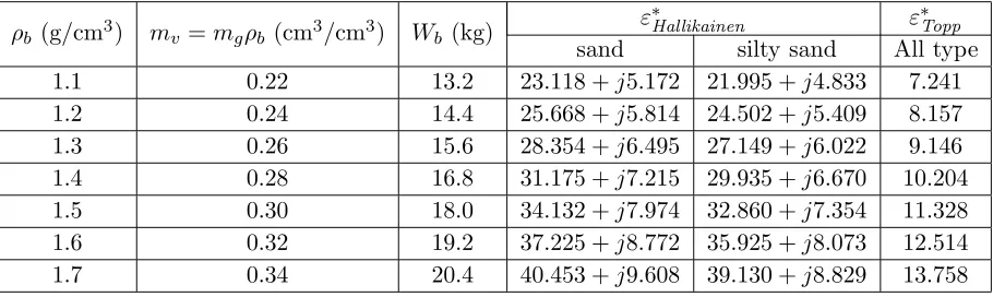
Using the wet soil empirical model given in Equations (2), (3), and (4), the soil dielectric permittivity is calculated for each soil density from 1.1 g/cm3 to 1.7 g/cm3 and presented in Table 1.
In Table 1, the dielectric permittivities for two types of soils are shown. It can be seen that the volumetric moisture content,mv, of soil varies with bulk density while the gravimetric moisture content, mg, remains because there was no water being added to the soil. It can also be observed that as bulk density increases, the permittivity also increases for both types of soil, which shows that as bulk density increases, soil, in general, will be able to absorb more energy that is radiated onto it. Notice that for Hallikainen’s model, sand has a higher permittivity for every soil density than Topp’s model. This defines that solids with larger soil particles in it are able to absorb more energy. Now that the dielectric permittivities are defined, the return loss can be determined by using equations below:
Γ = √
ε2− √ε1
√
ε2+√ε1
(10)
Table 1. Calculated complex dielectric permittivity for each soil type and bulk density.
ρb (g/cm3) mv =mgρb (cm3/cm3) Wb (kg) ε ∗
Hallikainen ε∗Topp
sand silty sand All type
RL(dB) = −20 log|Γ| (11)
where Γ is the reflection coefficient in numerical value; ε1 and ε2 are the real permittivity (dielectric
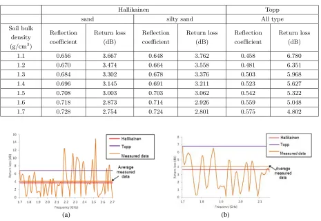
permittivity) of layer 1 and 2 of a structure, respectively;RLis the return loss in dB. The first layer is regarded as air, and the second layer is the soil sample. Given that the permittivity of air is 1 [5] and that the permittivity of soil is obtained from Table 1, the reflection coefficient and return loss values are calculated and tabulated in Table 2, which shows that with the increment of moisture content in soils, dielectric permittivity of the material will also increase as proved by [11, 12].
4.2. Soil Density Experiment Using Radio-Wave Reflection Method
Before starting the experiment, the equipments used were calibrated to check and eliminate possible system losses. Then, the calculated values of return loss using Hallikainen’s and Topp’s soil dielectric models are compared to the normalized measured data of sand at 1.2 g/cm3 as shown in Figure 3(a). It can be observed that the average normalized measured data are close to predicted value using Hallikainen’s model, about 5 dB, while Topp’s model is slightly over predicted at a value near 7 dB. It can also be seen at frequency higher than 2.2 GHz that the relative error between measured data and average measured data is higher. This has also been explained in a study by [15], that the return loss data measured gave lower relative error at 1.7 GHz than at 2.6 GHz. This is because lower frequency range has longer wavelength; therefore, the wave penetration in dielectric material is deeper. For this case, further analysis is done for frequency range from 1.7 GHz to 2.1 GHz, as shown in Figure 3(b). From Figure 3(b), the return loss for sand at 1.2 g/cm3 is regarded as an average of 4.2 dB, and this
Table 2. Reflection coefficient and return loss (dB) simulated using existing soil dielectric models.
Hallikainen Topp
sand silty sand All type
Soil bulk density (g/cm3)
Reflection coefficient
Return loss (dB)
Reflection coefficient
Return loss (dB)
Reflection coefficient
Return loss (dB)
1.1 0.656 3.667 0.648 3.762 0.458 6.780
1.2 0.670 3.474 0.664 3.558 0.481 6.351
1.3 0.684 3.302 0.678 3.376 0.503 5.968
1.4 0.696 3.145 0.691 3.211 0.523 5.627
1.5 0.708 3.003 0.703 3.062 0.542 5.322
1.6 0.718 2.873 0.714 2.926 0.559 5.048
1.7 0.728 2.754 0.724 2.801 0.575 4.802
(a) (b)
(a) (b)
Figure 4. Relationship of signal return loss in dB with soil density for (a) sand, (b) silty sand.
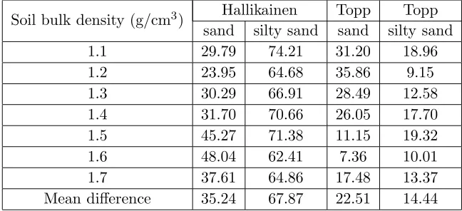
Table 3. Percentage difference between existing soil dielectric models with measured data.
Soil bulk density (g/cm3) Hallikainen Topp Topp sand silty sand sand silty sand
1.1 29.79 74.21 31.20 18.96
1.2 23.95 64.68 35.86 9.15
1.3 30.29 66.91 28.49 12.58
1.4 31.70 70.66 26.05 17.70
1.5 45.27 71.38 11.15 19.32
1.6 48.04 62.41 7.36 10.01
1.7 37.61 64.86 17.48 13.37
Mean difference 35.24 67.87 22.51 14.44
similar method is used for other densities for sand and silty sand from 1.1 g/cm3 to 1.7 g/cm3.
The relationship of return loss and soil density for both soil types is shown in Figure 4. Figure 4(a) and Figure 4(b) show how return loss (dB) of the signal changes with soil bulk density for sand and silty sand, respectively. For both soil types, Topp’s model gives the same decreasing trend as the soil density increases. This is because Topp’s model does not take into account the types of soil. On the other hand, Hallikainen’s model also decreases with density although just a little but gives a much lower value than Topp’s prediction. But it can be observed that the return loss value of silty sand is slightly increased as compared to sand. This is proved by [16] that soil with higher clay particles has lower dielectric permittivity. Therefore, since silty sand contains more clay particles than sand, it is expected to give a higher return loss value. To clearly see the difference, the measured soil return loss is compared to existing soil models, and the percentage differences are shown in Table 3. It can be seen that the calculated return loss using Hallikainen’s model gives smaller difference with the measured data than the ones calculated using Topp’s model. This is probably because the Topp’s equation is designed for all soil in general whereas Hallikainen’s model is more specific to each soil type.
Further in Figure 5, new soil density empirical models in terms of return loss (dB) are developed for each soil type as below.
DSAND = 0.310(RL)2−3,138(RL) + 9.215 (12)
DSilty = 0.034(RL)2−0.683(RL) + 4.404 (13)
(a) (b)
Figure 5. Comparison between predicted and actual soil density using three soil density models for (a) sand and (b) silty sand.
It can be seen in Figure 5(a), Hallikainen’s model gives a lower prediction of sand soil density value whereas Topp’s model over predicts the value, and some values are out of the range between 1.1 g/cm3
and 1.7 g/cm3. However, the new proposed model gives good predictions for every measurement. This
shows that the existing soil dielectric models might not be suitable to predict soil density using return loss approach. Most probably it is because the different method used to obtain the soil dielectric model. Since there is no soil density model being developed up till now, these two existing models are the closest ones to compare with. Even though some of the predicted values are out of the range, it can still be accepted as comparison because of the common parameters involved dielectric permittivity, soil type and moisture content. In Figure 5(b), Topp’s model gives a slightly lower prediction values while Hallikainen’s model still give some out of the range prediction values for silty sand soil density. The new proposed model, on the other hand, gives a very good prediction, closest to the actual value. To understand more the accuracy of the newly developed models, the error percentages for each soil model are shown in Table 4.
Table 4. Relative error of the predicted soil density between three soil models.
Soil density (g/cm3) Hallikainen Topp Novel/New soil density model
SAND Silty SAND SAND Silty SAND SAND Silty SAND
1.1 22.63 76.72 47.36 10.82 15.87 6.84
1.2 29.83 30.80 38.63 13.68 6.83 4.08
1.3 35.47 4.44 34.12 16.80 1.10 0.28
1.4 35.40 27.35 40.12 14.62 7.41 1.99
1.5 39.55 42.70 31.08 14.52 0.61 1.09
1.6 40.97 48.20 27.00 18.48 0.57 3.86
1.7 39.96 59.50 25.85 13.86 2.58 0.50
Mean relative error (%) 34.81 41.37 34.86 14.67 5.01 2.65
By referring to Table 4, it can be observed that Hallikainen’s model’s prediction gives about the same mean relative error as compared to Topp’s model for sand that is of average 34.81%. However, the newly developed soil density model gives the best relative error with an average of 5.01%. This shows that the new proposed soil density model is efficient enough to be used to predict soil density using the proposed technique. On the other hand, Hallikainen’s model gives the highest mean relative error of 41.39% for silty sand while Topp’s model gives a better mean relative error of 14.67%. Again, the new proposed model gives the best prediction with only 2.65% of mean relative error. Thus this strongly shows that the proposed model is indeed suitable for density estimation of soils.
(a) (b) (c)
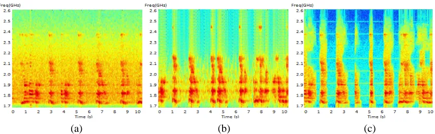
Figure 6. Results in time domain of spectrograms of soil, (a) highest density, (b) medium density, (c) lowest density.
produced in this study since they have been identified as a well-suited tool for observing sample condition. The spectrograms were produced based on the proposed developed models and related with [17]. The soil density estimation needs to be determined first with minimal data input such as soil type, return loss and reflection coefficient values within spectrum of frequencies. A spectrogram is proposed since it is visual representations of the spectrum of frequencies varying with time. It was calculated from the time signal using Equations (12) and (13) by using Matlab software, where this proposed method is a time-frequency distributions. It have been observed with a sweep frequency range from 1.7 GHz to 2.7 GHz. This process is a digital process where the data are digitally sampled in the time domain, then they are broken up into chunks, and to calculate the soil density of the frequency spectrum for each chunk. Each chunk then corresponds to a vertical line in measurement of soil density versus frequency for a specific moment in time.
Figure 6(a) shows the spectrograms of the highest density of soil. Figure 6(b) shows medium density whereas Figure 6(c) shows the lowest density. The spectrums or time plotted are looks laid side by side to form the image and looks slightly overlapped within the frequency range. It can be observed from the figures that the soil particles are highly detected in the low-frequency components, roughly below 2.1 GHz, due to high penetration of low frequency. For the higher frequency, roughly above 2.1 GHz, poor penetration of signal is obtained. The observation is found valid until 10 seconds. These trends are also valid for other soil densities as seen in Figure 6(b) and Figure 6(c). These results are expected to give much quicker soil density condition observation without causing damage to the soil structure and will benefit agricultural surveyors.
5. CONCLUSION
ACKNOWLEDGMENT
This project has been supported by the Graduate Research Assistant (GRA) scheme funded by Multimedia University with grant number IP20100104007, IP20110105021 and IP20120106008.
REFERENCES
1. Daniels, D., D. J. Gunton, and H. F. Scott, “Introduction to subsurface radar, radar and signal processing,” IEEE Proceedings F, Vol. 135, No. 4, 278–320, 1988.
2. Chen, B., Z. Hu, and W. Li, “Using ground penetrating radar to determine water content of rehabilitated coalmine soils treated by different methods,”10th International Conference on GPR, 513–516, 2004.
3. Conyers, B., “Moisture and soil differences as related to the spatial accuracy of ground penetrating radar amplitude maps at two archaeological test sites,” 10th International Conference on GPR, 435–438, 2004.
4. Malicki, M. A., J. Kokot, and W. M. Skierucha, “Determining bulk electrical conductivity of soil from attenuation of electromagnetic pulse,”International Agrophysics, Vol. 12, 181–183, 1998. 5. Daniels, D., Ground Penetrating Radar, 2nd Edition, The Institution of Electrical Engineers, UK,
2004.
6. Jol, H. M., Ground Penetrating Radar: Theory and Applications, Elsevier, Oxford, UK, 2009. 7. Pascale, S., P. Herve, and R. Dominique, “A non-destructive geophysical protocol for estimating
near-surface porosity, water content and water conductivity,” 10th International Conference on GPR, 723–726, 2004.
8. Behari, J., Microwave Dielectric Behaviour of Wet Soils, Anamaya Publishers, New Delhi, India, 2005.
9. O’Neill, N., “Multifrequency microwave radiometer measurements of soil moisture,” IEEE Transactions on Geoscience and Remote Sensing, Vol. 20, No. 4, 468–475, 1982.
10. Njoku, E. G. and D. Entekhabi, “Passive microwave remote sensing of soil moisture,” Journal of Hydrology, Vol. 184, No. 1, 101–130, 1995.
11. Topp, G. C., J. L. Davis, and A. P. Annan, “Electromagnetic determination of soil water content: Measurements in coaxial transmission lines,” Water Resources Research, Vol. 16, No. 3, 574–582, 1980.
12. Hallikainen, M. T., et al., “Microwave dielectric behavior of wet soil — Part 1: Empirical models and experimental observations,” IEEE Transactions on Geoscience and Remote Sensing, Vol. 23, No. 1, 25–34, 1985.
13. British Standard Institution, British Standard Methods of Test for Soils for Civil Engineering Purposes Part 2: Classification Tests,BSI, London, 1990.
14. Skolnik, M., Radar Handbook, 3rd Edition, McGraw Hill, USA, 2008.
15. Raja Abdullah, R. S. A., et al., “Evaluation of road pavement density using ground penetrating radar,”Journal of Environmental Science and Technology, Vol. 2, No. 2, 100–111, 2009.
16. Kutrubes, D. L., “Ground Penetrating Radar, Public Safety, and the FCC,” Symposium for the Applications of Geophysics to Environmental and Engineering Problems, San Antonio, TX, 2003. 17. Rangachari, S. and P. C. Loizou, “A noise-estimation algorithm for highly non-stationary