A Novel Image Formation Method for Electromagnetic Vortex SAR
with Orbital-Angular-Momentum
Yue Fang1, Jie Chen1, Pengbo Wang1, *, Chunsheng Li1, and Wei Liu2
Abstract—Electromagnetic (EM) vortex wave carrying orbital angular momentum (OAM) has
attracted a lot of attention in radar imaging, due to its potential capability of new degree of freedom for information modulation. Most existing OAM-based radar imaging methods require abundant OAM modes to realize the azimuth resolution. Switching between the OAM modes frequently increases the burden of radar antenna and the complexity of beam steering. In this paper, a novel electromagnetic vortex synthetic aperture radar (EMV-SAR) model with equivalent squint imaging is established. The geometrical model and echo signal model are derived correspondingly. By analyzing the echo signal model, amplitude and phase modulation introduced by the OAM affect the azimuth focusing, and traditional imaging algorithms are no longer applicable. Hence, a novel image formation method based on the traditional Chirp-Scaling (CS) algorithm is proposed for the EMV-SAR. The amplitude weighting function and phase modulation function are derived accurately, and high-precision focusing processing is achieved by modified CS algorithm. Point targets simulation results validate that the image focusing performance can be improved significantly using the proposed algorithm.
1. INTRODUCTION
In the past two decades, research on electromagnetic (EM) vortex carrying orbital angular momentum (OAM) has received more and more attention due to its particular physical property [1–4], which possesses helical phase fronts, providing unique methods for information acquisition and modulation. For the time being, EM vortex with OAM has found a wide variety of applications in fields including beam formation [5–8], electromagnetic wave detection [9], and wireless communication [10]. In [3, 10], the ability of enhancing channel capacity and anti-interference by transmitting OAM waves is validated. In [11, 12], the OAM division multiplexing technique information transmission is independently verified by observing a demultiplexing interferometer output ports, verifying that high-capacity and high speed communication are achieved by the OAM.
In recent years, EM vortex has been applied in radar imaging area. As shown in [13], EM vortex has the potential to achieve the azimuth resolution of the radar target. The approximate duality relation between OAM mode number and azimuth angle is firstly analyzed. Subsequently, in [14, 15], the echo signal models of both multiple-in-multiple-out (MIMO) and multiple-in-single-out (MISO) modes are derived based on uniform concentric arrays (UCA), and two-dimensional (2-D) target imaging results are obtained by using fast Fourier transform (FFT) and back-projection (BP) methods. In [16], main-lobe convergence of vortex beam is investigated. Several concentric circular arrays are employed to adjust the directivity of the main-lobe and reduce the high side-lobe levels. A beam steering method is proposed in [17] with UCA, and 2-D target imaging is achieved by an lp regularized least-squares algorithm. In [18], two targets in the same range gate are tracked, and the azimuth and elevation angles are obtained by using three different topological charges.
Received 17 January 2019, Accepted 1 March 2019, Scheduled 28 June 2019
* Corresponding author: Pengbo Wang ([email protected]).
1 School of Electronic and Information Engineering, Beihang University, Beijing 100191, China. 2 Electronic and Electronic
However, the above mentioned imaging methods are all based on a fixed radar system, where the antenna system is static, and a number of OAM modes are needed for its effective operation. In fact, changing the OAM mode number frequently imposes more constraints on the radar antenna system and increases its complexity. The generation of OAM mode number is limited by the number of antenna array elements [19], which may increase the requirement of system design in the case of high resolution. Fortunately, SAR system operation mode makes it possible to possess the azimuth resolution, simply by the relative motion between radar and targets. Moreover, the high capacity of information modulation by the OAM [11, 12] can be introduced into SAR fields, benefiting the information-rich SAR and targets detection. Furthermore, the unique doughnut-like radiation distribution of EM vortex waves can be utilized to enhance the coverage performance of SAR system. Hence, in this paper, the EM vortex waves are introduced into the SAR imaging field, where the radar antenna is moving along the flight direction. The OAM mode is fixed in the whole flight duration, significantly reducing the hardware complexity of the system. The geometric model of SAR carrying OAM is established, and the echo signal model is derived correspondingly. Based on the newly proposed signal model, a novel SAR imaging algorithm with OAM is proposed, following the approach of the traditional Chirp-Scaling (CS) algorithm [20].
The rest of this paper is organized as follows. Section 2 gives the imaging model and echo signal model of the proposed electromagnetic vortex synthetic aperture radar (EMV-SAR). The new imaging algorithm for EMV-SAR is proposed in Section 3. Numerical simulation results are presented in Section 4. Conclusion and discussion are provided in Section 5.
2. IMAGING MODEL AND ECHO SIGNAL MODEL OF EMV-SAR
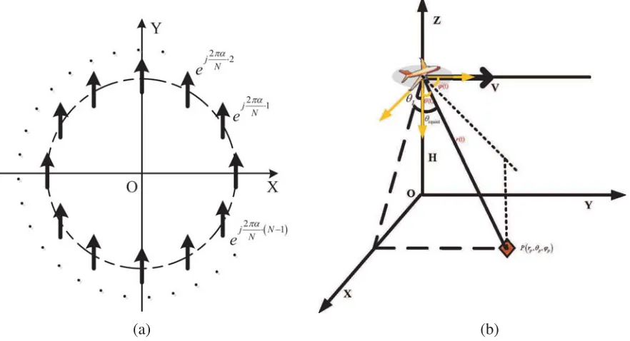
In the proposed EMV-SAR, a single UCA is adopted as the transmit and receive (T/R) antenna to generate EM vortex waves carrying the OAM, as shown in Fig. 1. N omnidirectional antennas are uniformly-spaced around the circle with radius a, each with a phase shift of δΦn = 2πnα/N,
n = 0,1, ..., N −1, where α is the OAM mode number. The geometry of the proposed EMV-SAR is shown in Fig. 1(b). The airplane flies along the Y-axis direction, at a constant height H and velocity
V. Targets on the ground are illuminated by EM vortex waves within the beam-width covered area.
(a) (b)
Figure 1. Geometry of EMV-SAR: (a) the model of the employed UCA based antenna system, and
(a) (b)
Figure 2. Imaging mode of EMV-SAR: (a) sketch of system stripmap mode, and (b) principle of
synthetic aperture.
The imaging mode is illustrated in Fig. 2. EM vortex pulses are transmitted and received at the same pulse repetition interval (PRI), carrying a fixed OAM mode. The range resolution is achieved by transmitting the broadband linear frequency modulated (LFM) signal and using the matched filtering process. According to the principle of synthetic aperture, shown in Fig. 2(b), azimuthal resolution can be realized by accumulating illumination in the azimuthal direction.
According to the geometry of EMV-SAR and characteristics of T/R antennas, for an arbitrary point targetp(rp, θp, ϕp) in the free space, the echo of LFM signal with OAM based on the model shown in Fig. 1(a) is given in Equation (1), modified from [15],
secho(τ, t) = σ
(rp, θp, ϕp)
r2(t) wa(t−tc)wr
τ −2r(t) c
exp
jπKr
τ −2r(t) c
2
·exp
−j2πfc2r(t)
c
J2
α(kasinθ(t)) exp{j2αϕ(t)} (1)
whereσ(rp, θp, ϕp) is the radar cross section (RCS) of the targetp(rp, θp, ϕp), and it is a constant during the whole sythetic aperture, unless the OAM mode is changeable [21]. tc is the moment of the Doppler centroid;fc represents the carrier frequency;cis the speed of light; br is the LFM ratio;wa(·) andwr(·) are the envelopes of azimuth and range; Jα(·) denotes the Bessel function of the first kind, which is shown in a squared form due to the effect of both transmission and reception; k=ω/c represents the wave number; andθ(t) is the elevation angle, which is time-varying due to the relative motion between antenna and target.
The two items Jα2(kasinθ(t)) and exp{j2αϕ(t)} in Equation (1) affect the weighting of antenna pattern and phase modulation, respectively. Their effect on image formation will be analyzed in Section 3. θ(t) is given by,
θ(t) =acos −H
r(t)
(2)
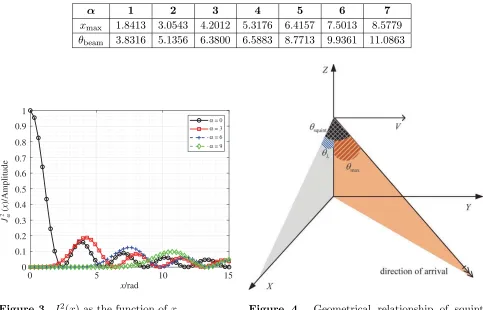
As shown in Fig. 3, the value of Jα2(x) depends on the OAM modeα and x, wherex=kasinθ in our proposed echo signal model, indicating that the elevation angle θcan be linked tox. Whenα= 0, the main-lobe of Jα2(x) is located at x= 0, which is understandable in the traditional SAR operation mode. However, in EMV-SAR, whereα is nonzero, the main-lobe will deviate from the axial direction. So the main-lobe direction does not have the side-looking orientation any more. In the meantime, the beamwidth of the main-lobe also varies via different OAM modes.
Fortunately, the value of OAM mode α here is a constant, and the main-lobe direction and beamwidth can be calculated without difficulty. Table 1 gives the location of main-lobe xmax and its
Table 1. Main-lobe location and beam width for different OAM modes.
α 1 2 3 4 5 6 7
xmax 1.8413 3.0543 4.2012 5.3176 6.4157 7.5013 8.5779
θbeam 3.8316 5.1356 6.3800 6.5883 8.7713 9.9361 11.0863
0 5 10 15
x/rad
1
0.9
0.8
0.7
0.6
0.5
0.4
0.3
0.2
0.1
0
J
(
x
)/Amplitude
2 α
α = 0
α = 3
α = 6
α = 9
Figure 3. Jα2(x) as the function ofx. Figure 4. Geometrical relationship of squint
angle θsquint.
θbeam of main-lobe can be derived as follows,
θmax = arcsin
x
max
ka rad (3)
θbeam = 0.886·arcsin
zrignt−zleft
ka
rad (4)
wherezrignt andzleft denote the right zero point and left zero point of the main-lobe, respectively.
The direction of main-lobe determines the value of antenna squint angle, whose geometrical relationship is illustrated in Fig. 4.
The value of squint angleθsquint can be calculated as,
θsquint= arccos (cosθL·cosθmax) (5)
The target azimuth angleϕin exp{j2αϕ(t)} is also time-varying within the illumination duration, and it is given by
ϕ(t) =atan yp−vt
R2
0−H2
(6)
where yp = rpsinθpcosϕp is the Y-axis coordinate of target. r(t) = R2
0+V2t2 is the slant range
between antenna and target, where R0 =
r2
psin2θpcos2ϕ
p+H2 represents the nearest slant range
between antenna and target, and H is the height of platform.
3. IMAGE FORMATION METHOD FOR EMV-SAR
In this section, the limitation of traditional SAR image formation method is described firstly by analyzing the characteristics of the EMV-SAR echo signal model. A novel image formation method for EMV-SAR based on the traditional Chirp-Scaling algorithm is proposed subsequently.
3.1. Limitation in Traditional Imaging Algorithms
The traditional SAR echo signal model is given as follows
secho tra(τ, t) = σ
(r, θ, ϕ)
r2 wa(t−tc)wr
τ−2r c
exp
jπKr(τ −2r/c)2
·exp
−j2πfc2r
c
(7)
Traditional imaging methods are based on the two-dimensional (2-D) coupling relationship between range cell migration and azimuth exponent phase, given as 2r/c and 4πr(t)/λ, respectively. The newly introduced items by OAM destroy such a relationship. For the additional phase item, exp{j2αϕ(t)}, it appears as a space-variant variable in the azimuthal direction according to Equation (6). Such an OAM phase term will affect the azimuthal compression as a result and invalidate the traditional imaging algorithms. Hence, phase compensation is necessary for the azimuthal compression processing.
Moreover, the additional amplitude modulation on the antenna pattern weighting needs to be considered. According to Fig. 3, the received signal will be weighted by an asymmetric pattern, which leads to the imbalance of azimuthal energy and deterioration of azimuthal focusing. Therefore, amplitude modulation should likewise be corrected in the image formation process.
Based on the above analysis, traditional SAR imaging algorithms cannot be used for EMV-SAR directly. The new items introduced by OAM mainly affect the azimuthal focusing. Meanwhile, considering that targets in the same range direction are weighted by the same antenna pattern and share a common phase history, the correction processing can be performed in the range-Doppler (R-D) domain after range compression.
3.2. Image Formation Method of EMV-SAR
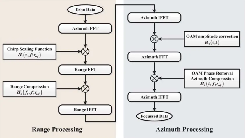
A flowchart of the proposed imaging algorithm for EMV-SAR is shown in Fig. 5. It consists of four main steps: chirp scaling processing, range compression, correction of antenna pattern weighting, i.e., OAM amplitude modulation, and OAM phase modulation removal and azimuth compression.
According to the traditional Chirp-Scaling algorithm [20], in the first step, chirp scaling processing is achieved in the R-D domain, and the echo signal in the R-D domain is multiplied by the function
H1(τ, f;rref), given in Equation (8), normalising range migration for all targets at different ranges and
aligning them to the reference curvature trajectory.
H1(τ, f;rref) = exp
−jπbr(f;rref)Cs(f)[τ−τref(f)]2
(8)
where the derivation of br(f;rref), Cs(f), andτref(f) can be found in [20].
Then, FFT in range direction is applied, and the signal is transformed into the 2-D domain. After that, range cell migration correction (RCMC) and range focus including secondary range compression (SRC) are achieved by H2(fτ, f;rref) in the 2-D domain.
After the two steps, the signal of all targets is rectilinear, with OAM amplitude weighting and phase modulation to be removed in the third step.
The OAM amplitude can be approximated whenx1,J2
α(x) by [15],
J2
α(x)≈ 2
πxcos2
x−απ
2 −
π
4 (9)
which can be further simplified as,
J2
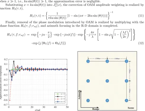
α(x)≈ πx1 [1−sin (απ−2x)] (10) The approximation error introduced in Equation (9) is illustrated in Fig. 6. It can be seen that when x1, i.e., kasin(θ(t))1, the approximation error is negligible.
Substitutingx=kasin(θ(t)) into Jα2(x), the correction of OAM amplitude weighting is realized by functionH3(τ,t),
H3(τ,t) =
1
πkasin (θ(t))[1−sin (απ−2kasin (θ(t)))] −1
(11)
Finally, removal of the phase modulation introduced by OAM is realized by multiplying with the phase function H4(τ, f;rref), and azimuth focusing in the R-D domain is completed.
H4(τ, f;rref) = exp
−jα·π
2
·exp{−jαφ(f)} ·exp ⎧ ⎨ ⎩−j
4π
λ r
⎡
⎣1−sinϕ
1−
λf
2v 2⎤
⎦ ⎫ ⎬ ⎭
·exp{j[Θ1(f) + Θ2(f)]} (12)
0 10 20 30
x/rad
0.2
0.1
0
-0.1
-0.2
-0.3
-0.4
-0.5
-0.6
-0.7
Approximation error/Amplitude
α = 0
α = 3
α = 6
α = 9
40 50
Figure 6. Approximation error in Equation (9). Figure 7. Geometrical layout of the considered
Here,φ(f) is the frequency domain expression of azimuth angleϕ(t), shown in Equation (1), and
Θ1(f) =
4π
c2br(f;rref) [1 +Cs(f)]Cs(f)
r sinϕ
sinϕref −rref 2
(13)
Θ2(f) = 2πrf·cosϕ/v (14)
4. SIMULATION RESULTS AND DISCUSSION
In this section, echo signal simulation and imaging result of point targets are provided. The considered scene is shown in Fig. 7, where nine point targets are distributed as a 3×3 matrix, and targets RCSs are considered as constants. The spacing of adjacent targets is labeled accordingly.
Simulation parameters are listed in Table 2.
Table 2. Simulation parameters.
Parameter Value Unit Antenna center angle 35 deg
OAM mode number 7 -UCA radius 30λ m
Bandwidth 100 MHz Pulse width 10 µs Sampling rate 140 MHz Pulse repetition frequency 2000 Hz
Flight velocity 250 m/s Scene center slant range 30000 m
According to the analysis in Section 2, the elevation angle θmax and 3 dB beamwidth θbeam of
main-lobe can be calculated as
θmax = arc sin
x
max
ka ≈0.2900 rad (15)
θbeam = 0.886·arc sin
zrignt−zleft
ka
≈0.3354 rad (16)
(a) (b)
500 1000 1500 2000 Azimuth/Samples
2500 3000 3500 4000 500 1000 1500 2000
Azimuth/Samples
2500 3000 3500 4000 14
12
10
8
6
4
2
Amplitude Weighting
10
9
8
7
6
5
4
Amplitude Weighting 3
2
1
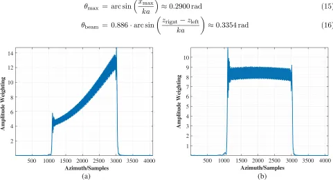
Figure 8. Azimuth antenna pattern weighting before and after the proposed processing: (a) weighting
The value of squint angleθsquint is
θsquint= arccos (cosθL·cosθmax) = 0.6682 rad (17)
It means that EMV-SAR operates at the squint angleθsquint of 0.6682 rad with a beamwidthθbeam
of 0.3354 rad.
Here, the targets numbered 1, 5, and 9 are selected to validate the performance of the proposed method. In order to demonstrate the validity of the proposed amplitude correction method for EMV-SAR, comparisons of azimuth antenna weighting in the scene central range gate before and after the amplitude correction are shown in Fig. 8.
As shown in Fig. 8(a), targets are weighted by an asymmetrical pattern in the azimuthal direction. This irregular weighting pattern will lead to azimuth defocusing and need to be corrected. The result of azimuthal pattern correction is shown in Fig. 8(b), where it can be observed that the amplitude envelope is corrected to be nearly uniform along the azimuthal direction, demonstrating the effectiveness of the proposed amplitude correction processing.
(a)
(b) 200 400 600 800
Range/Samples expanded by 128
1000 1200 1400 1600 1800 2000
Point Target 1
(c)
Range Profile Azimuth Profile
Point Target 5 Range Profile Azimuth Profile
Point Target 9 Range Profile Azimuth Profile
200 400 600 800
Azimuth/Samples expanded by 128
1000 1200 1400 1600 1800 2000 200 400 600 800
Azimuth/Samples expanded by 128
1000 1200 1400 1600 1800 2000 200 400 600 800
Azimuth/Samples expanded by 128
1000 1200 1400 1600 1800 2000
200 400 600 800
Range/Samples expanded by 128
1000 1200 1400 1600 1800 2000
200 400 600 800
Range/Samples expanded by 128
1000 1200 1400 1600 1800 2000
500 1000 1500 2000
Range/Samples expanded by 128
2500 3000 3500 4000
500 1000 1500 2000
Range/Samples expanded by 128
2500 3000 3500 4000
500 1000 1500 2000
Range/Samples expanded by 128
2500 3000 3500 4000 0 -10 -20 -30 -40 -50 -60 Amplitude/dB 0 -10 -20 -30 -40 -50 -60 Amplitude/dB 0 -10 -20 -30 -40 -50 -60 Amplitude/dB
500 1000 1500 2000
Azimuth/Samples expanded by 128
2500 3000 3500 4000
500 1000 1500 2000
Azimuth/Samples expanded by 128
2500 3000 3500 4000
500 1000 1500 2000
Azimuth/Samples expanded by 128
2500 3000 3500 4000 0 -10 -20 -30 -40 -50 -60 Amplitude/dB 0 -10 -20 -30 -40 -50 -60 Amplitude/dB 0 -10 -20 -30 -40 -50 -60 Amplitude/dB
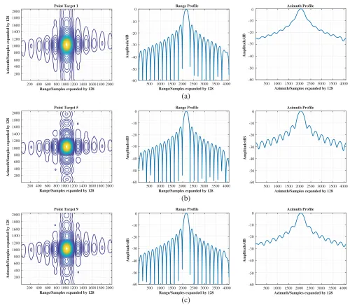
Figure 9. Imaging result of targets 1, 5, and 9, based on the traditional algorithm. (a) Point Target
Figure 9 shows the imaging results of the traditional chirp scaling algorithm, which does not consider the OAM effect. The corresponding results by the proposed algorithm are shown in Fig. 10.
(a)
(b)
Point Target 1
(c)
Range Profile Azimuth Profile
Point Target 5 Range Profile Azimuth Profile
Point Target 9 Range Profile Azimuth Profile
200 400 600 800
Range/Samples expanded by 128
1000 1200 1400 1600 1800 2000
200 400 600 800
Range/Samples expanded by 128
1000 1200 1400 1600 1800 2000
200 400 600 800
Range/Samples expanded by 128
1000 1200 1400 1600 1800 2000 200
400 600 800
Azimuth/Samples expanded by 128
1000 1200 1400 1600 1800 2000 200 400 600 800
Azimuth/Samples expanded by 128
1000 1200 1400 1600 1800 2000 200 400 600 800
Azimuth/Samples expanded by 128
1000 1200 1400 1600 1800 2000
500 1000 1500 2000
Range/Samples expanded by 128
2500 3000 3500 4000 0 -10 -20 -30 -40 -50 -60 Amplitude/dB
500 1000 1500 2000
Azimuth/Samples expanded by 128
2500 3000 3500 4000
0 -10 -20 -30 -40 -50 -60 Amplitude/dB 0 -10 -20 -30 -40 -50 -60 Amplitude/dB 0 -10 -20 -30 -40 -50 -60 Amplitude/dB 0 -10 -20 -30 -40 -50 -60 Amplitude/dB 0 -10 -20 -30 -40 -50 -60 Amplitude/dB
500 1000 1500 2000
Range/Samples expanded by 128
2500 3000 3500 4000 500 1000 1500 2000
Azimuth/Samples expanded by 128
2500 3000 3500 4000
500 1000 1500 2000
Range/Samples expanded by 128
2500 3000 3500 4000 500 1000 1500 2000
Azimuth/Samples expanded by 128
2500 3000 3500 4000
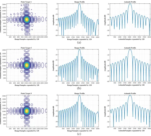
Figure 10. Imaging result of targets 1, 5, and 9, based on the proposed algorithm. (a) Point Target 1.
(b) Point Target 5. (c) Point Target 9.
According to Fig. 9, the focus in azimuth is not satisfactory. Azimuth side-lobes are elevated entirely, and the target in the near range is worse than that at the far range, while for the proposed method, as shown in Fig. 10, it is capable of effective 2-D focusing of the whole scene. All of targets are well focused, and 2-D side-lobes are decreased.
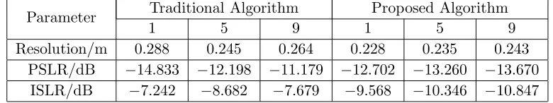
Table 3 gives the performance comparison of the azimuthal impulse response, including resolution, peak side-lobe ratio (PSLR), and integrated side-lobe ratio (ISLR).
It can be seen that the azimuth resolution of proposed method, 0.235 m, is superior to the result of the traditional chirp scaling algorithm, 0.245 m, and not only the near range target is well focused, but also the far range one. For the center point, target number 5, the PSLR and ISLR stay below
Table 3. Comparison of imaging performance.
Parameter Traditional Algorithm Proposed Algorithm
1 5 9 1 5 9
Resolution/m 0.288 0.245 0.264 0.228 0.235 0.243 PSLR/dB −14.833 −12.198 −11.179 −12.702 −13.260 −13.670
ISLR/dB −7.242 −8.682 −7.679 −9.568 −10.346 −10.847
−8.682 dB, respectively.
Based on the results in Table 3, we can say that focusing of the whole scene of EMV-SAR has been achieved by the proposed algorithm successfully, while the traditional chirp scaling algorithm is not applicable. The amplitude weighting and phase modulation of OAM mainly affect the azimuth phases of targets, which would make a direct contribution to the azimuth defocusing, especially for the PSLR and ISLR. The proposed imaging formation method tackles these problems. The asymmetrical amplitude weighting is corrected well, and the 2-D compressing results validate that the influence of OAM formulation is removed. Given the above, our proposed imaging method is capable of EMV-SAR echo imaging processing.
5. CONCLUSIONS
A novel SAR imaging model based on EM vortex waves has been proposed, which employs a single UCA to generate the required EM vortex waves. The broadband LFM signal is transmitted and received to acquire the wide bandwidth in the range direction and realize the range resolution, while the azimuth resolution is obtained by transmitting the equally spaced pulses at a certain PRI and accumulating illumination in the azimuthal direction. The corresponding geometrical structure and echo signal model are established. As shown, the introduction of OAM leads to azimuthal antenna pattern weighting and phase modulation, which mainly affect the azimuthal compression processing. A 2-D target imaging algorithm is derived based on principle of the traditional Chirp-Scaling algorithm, with amplitude correction and phase compensation taken into account. As demonstrated by simulation results, EM vortex waves with OAM can be utilized to achieve a well-focused image for the whole scene, with significantly improved azimuthal focussing effects.
However, further research is needed on two issues. Since the amplitude weighting of the Bessel function is independent of target slant range, it will bring in additional weighting in the range direction, leading to asymmetric side-lobe of the range profile. Another issue is the existence of zero-zone in the range weighting when the width is large enough, which will limit the range width of the scene.
ACKNOWLEDGMENT
This work was supported by the National Natural Science Foundation of China (Grant No. 61628101) and the Innovation Foundation of Aerospace Science and Technology of Shanghai (Grant No. SAST2016029).
REFERENCES
1. Wang, J., J. Y. Yang, I. M. Fazal, N. Ahmed, Y. Yan, H. Huang, Y. Ren, Y. Yue, S. Dolinar, and M. Tur, “Terabit free-space data transmission employing orbital angular momentum multiplexing,” Nature Photonics, Vol. 6, No. 7, 488–496, 2012.
3. Mahmouli, F. E. and S. D. Walker, “4-Gbps uncompressed video transmission over a 60-GHz orbital angular momentum wireless channel,”IEEE Wireless Communications Letters, Vol. 2, No. 2, 223– 226, 2013.
4. Mohammadi, S., L. K. Daldorff, J. E. Bergman, R. L. Karlsson, B. Thid´e, K. Forozesh, T. D. Carozzi, and B. Isham, “Orbital angular momentum in radio — A system study,” IEEE Transactions on Antennas and Propagation, Vol. 58, No. 3, 565–572, 2010.
5. Bai, Q., A. Tennant, and B. Allen, “Experimental circular phased array for generating OAM radio beams,”Electronics Letters, Vol. 50, No. 20, 1414–1415, 2014.
6. Barbuto, M., F. Trotta, F. Bilotti, and A. Toscano, “Circular polarized patch antenna generating orbital angular momentum,”Progress In Electromagnetics Research, Vol. 148, 23–30, 2014. 7. Mao, F., T. Li, Y. Shao, J. Yang, and M. Huang, “Orbital angular momentum radiation from
circular patches,” Progress In Electromagnetics Research Letters, Vol. 61, 13–18, 2016.
8. Mao, F., M. Huang, T. Li, J. Zhang, and C. Yang, “Broadband generation of orbital angular momentum carrying beams in RF regimes,” Progress In Electromagnetics Research, Vol. 160, 19– 27, 2017.
9. Cano, E., B. Allen, Q. Bai, and A. Tennant, “Generation and detection of OAM signals for radio communications,”Antennas and Propagation Conference (LAPC), 637–640, 2014.
10. Tamburini, F., E. Mari, A. Sponselli, B. Thid´e, A. Bianchini, and F. Romanato, “Encoding many channels in the same frequency through radio vorticity: First experimental test,” New Journal of Physics, Vol. 14, No. 3, 033001, 2011.
11. Gibson, G., J. Courtial, M. J. Padgett, M. Vasnetsov, V. Pas’ko, S. M. Barnett, and S. Franke-Arnold, “Free-space information transfer using light beams carrying orbital angular momentum,” Optics Express, Vol. 12, No. 22, 5448–5456, 2004.
12. Gatto, A., M. Tacca, P. Martelli, P. Boffi, and M. Martinelli, “Free-space orbital angular momentum division multiplexing with Bessel beams,” Journal of Optics, Vol. 13, No. 6, 064018, 2011.
13. Guo, G., W. Hu, and X. Du, “Electromagnetic vortex based radar target imaging,” Journal of National University of Defense Technology, Vol. 35, No. 6, 2013.
14. Liu, K., Y. Cheng, Z. Yang, H. Wang, Y. Qin, and X. Li, “Orbital-angular-momentum-based electromagnetic vortex imaging,” IEEE Antennas and Wireless Propagation Letters, Vol. 14, 711– 714, 2015.
15. Liu, K., Y. Cheng, X. Li, H. Wang, Y. Qin, and Y. Jiang, “Study on the theory and method of vortex-electromagnetic-wave-based radar imaging,” IET Microwaves Antennas and Propagation, Vol. 10, No. 9, 961–968, 2016.
16. Yuan, T., H. Wang, Y. Qin, and Y. Cheng, “Electromagnetic vortex imaging using uniform concentric circular arrays,”IEEE Antennas and Wireless Propagation Letters, Vol. 15, 1024–1027, 2016.
17. Yuan, T., Y. Cheng, H. Wang, and Y. Qin, “Beam steering for electromagnetic vortex imaging using uniform circular arrays,”IEEE Antennas and Wireless Propagation Letters, Vol. 16, 704–707, 2017. 18. Tang, B., J. Bai, and K.-Y. Guo, “Bi-target tracking based on vortex wave with orbital angular
momentum,” Progress In Electromagnetics Research C, Vol. 74, 123–129, 2017.
19. Thid´e, B., H. Then, J. Sj¨oholm, K. Palmer, J. Bergman, T. Carozzi, Y. N. Istomin, N. Ibragimov, and R. Khamitova, “Utilization of photon orbital angular momentum in the low-frequency radio domain,” Physical Review Letters, Vol. 99, No. 8, 087701, 2007.
20. Raney, R. K., H. Runge, R. Bamler, I. G. Cumming, and F. H. Wong, “Precision SAR processing using chirp scaling,” IEEE Transactions on Geoscience and Remote Sensing, Vol. 32, No. 4, 786– 799, 1994.