_____________________________________________________________________________________________________
www.sciencedomain.org
On Which Variable(s) Should We Condition to
Remove Confounding Bias?
Eyal Shahar
1*and Doron J. Shahar
21
Department of Epidemiology and Biostatistics, Mel and Enid Zuckerman College of Public Health, University of Arizona, USA. 2
Department of Mathematics, College of Science, University of Arizona, USA.
Authors’ contributions
This work was carried out in collaboration between the two authors, which included many discussions and the drawing of causal diagrams. Author ES wrote the first draft of the manuscript. Author DJS offered critical revisions. Both authors read and approved the final manuscript.
Article Information
DOI: 10.9734/BJMMR/2015/19751 Editor(s): (1) Crispim Cerutti Junior, Department of Social Medicine, Federal University of Espirito Santo, Brazil. Reviewers: (1) A. Papazafiropoulou, Department of Internal Medicine and Diabetes Center, Tzaneio General Hospital of Piraeus, Greece. (2)F. E. Okwaraji, University of Nigeria, Nigeria. (3) Behnam Sharif, Department of Community Health Sciences, University of Calgary, Canada. Complete Peer review History:http://sciencedomain.org/review-history/10476
Received 25th June 2015 Accepted 21st July 2015 Published 11th August 2015
ABSTRACT
Using causal diagrams and an axiomatization of causality, we examined the well-known claim that conditioning on confounders (“adjustment” for confounders) is sufficient to remove confounding bias. We show that this advice is poorly stated and is incomplete. To remove confounding bias, it is necessary to condition on three types of variables, none of which is a confounder. Conditioning on one of them, however, leads to an interesting form of colliding bias, which in turn, can be removed by conditioning on two other types of variables.
Keywords: Causal diagrams; axioms of causality; confounding bias; colliding bias; conditioning.
1. INTRODUCTION
By definition, a confounder (C) is any shared cause of the exposure (E) and the disease (D),
path ED alone, but also from the confounding path ECD – an open (associational) path between the exposure and the disease.
It is widely believed that conditioning on C (“adjustment” for C) is sufficient to remove confounding bias due to C. We examined the validity of this claim under axioms of causality.
2. RELEVANT AXIOMS
Scientific inference, like any kind of inference, must rely on axioms – a set of primary premises that cannot be derived from other premises. Surprisingly, the voluminous literature in philosophy of science does not contain an elaborated axiomatization of causality, except for the well-known clash between determinism and indeterminism [2].
We previously proposed a set of axioms about indeterministic causation [3], four of which are relevant here:
All causation operates between time point variables: a variable at one time (e.g., A0) affects a variable at a later time (e.g., Y1).
If AY, then AiYj for any i and j where j>i
A direct effect exists only on the dt scale of time, where dt is an infinitesimal time interval (as in Newton’s calculus): A0Y0+dt;A0A0+dt. Informally: there is no “time travel” of an effect.
A variable at one time (e.g., A0) affects that variable at any future time (e.g., A1): A0 A0+dt…A1-dtA1
Notice two important derivations: First, any arrow between two time point variables is just a convenient abbreviation for causal paths on the dt scale of time. Second, the effect of A on Y
should be estimated for a specified time interval between the two variables.
3. BLOCKING CONFOUNDING PATHS
In light of the axioms, the causal structure in Fig. 1 is an oversimplification. There are no generic variables such as C, E, and D – only time point variables, each taking the value of some property at a distinct time. Given the causal ordering of C, E, and D (C is a cause of E; E is a cause of D), a sequential subscript may denote a time point for each variable: C0, E1, D2. Without losing generality, we assume throughout that the subscript “0” denotes a property at its inception.
To estimate the effect E1D2 and remove confounding bias, we may block the path E1C0D2 by conditioning on C0 (Fig. 2).
Conditioning, denoted by a box, dissociates a variable from all other variables, as denoted by crossing lines over surrounding arrows. After conditioning on C0, the (conditional) association between E1 and D2 does not include the unwanted contribution of the confounding path.
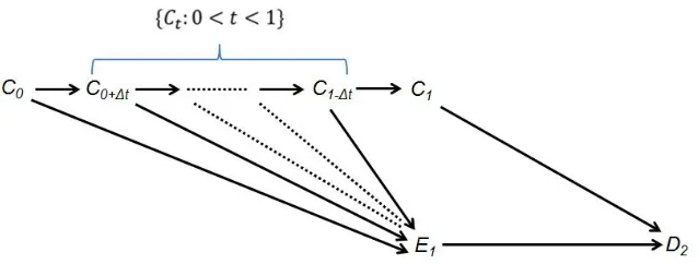
C0, however, indicates the C-property at just one time point before E1. Between t=0 and t=1, there are an infinite number of interim Ct variables (0<t<1), as shown in Fig. 3. Two C-variables that are close to C0and C1 are labeled, respectively, C0+Δt and C1-Δt.
In accord with the axioms of causality, the set of interim Ct form a causal path between C0 and C1 (C0C0+Δt…C1-ΔtC1), and each of these variables is also a cause of E1. Therefore, there is a continuum of Ct, each of which creates a unique confounding path: E1CtC1D2 (Fig. 3). The so-called confounder C is actually a set of an infinite number of confounders.
Fig. 2. Blocking the confounding path
Fig. 4 shows what happens after conditioning on C0. One confounding path is indeed blocked, as we already saw in Fig. 2, but an infinite number of paths, E1CtC1D2, remain open.
Fig. 4 leads to another conclusion: let Cj be a member of {Ct: 0<t<1}. Then, the shorter the time interval between Cj and C1, the smaller the set of confounding paths that remain open after conditioning on Cj. Therefore, if we have to choose between conditioning on Ciand Cj (i<j<1), it is better to condition on Cj (less bias will remain).
Most important, however, is the following conclusion:
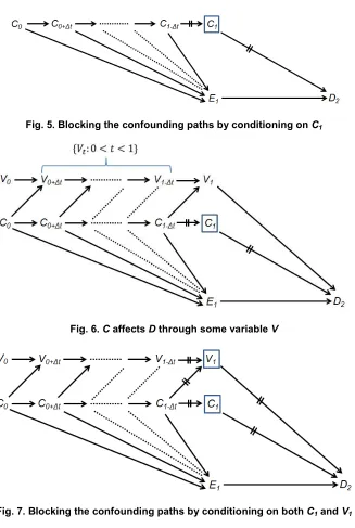
Rather than conditioning on C0 or any other confounder, Cj (j<1), we should condition on C1 – the variable that coincides with the exposure variable E1 (Fig. 5). Since C1 is located on all preceding confounding paths, conditioning on this variable will block them all. But C1 is not a confounder! It is not a cause of E1.
Conditioning on C1 will not suffice, however, if C0 affects D2 not only through subsequent C -variables, but also through other -variables, such as V (Fig. 6). In that case, an infinite number of confounding paths, E1Ct1Vt2V1D2, where 0<t1<t2<1, still remain open. To remove all confounding due to C-variables, we have to condition on V1 as well (Fig. 7). Notice that V1 is not a confounder, either. It is a cause of D2, but not a cause of E1.
Fig. 3. An infinite number of confounding paths due to C-variables
Fig. 5. Blocking the confounding paths by conditioning on C1
Fig. 6. C affects D through some variable V
Fig. 7. Blocking the confounding paths by conditioning on both C1 and V1
4. CONFOUNDING BY PREVIOUS
EXPOSURE VARIABLES
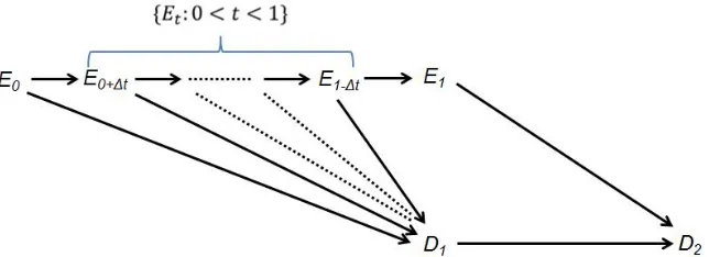
Although not widely recognized, E-variables before E1 are confounders too. Unless the effect of E on D is precisely null, each of them is not only a cause of E1, but also a cause of D2 through D1 (Fig. 8). Just like Ct and Vt, the Et variables collectively create an infinite number of confounding paths (E1EtD1D2), which make an unwanted contribution to the association between E1and D2.
How can we block these paths?
Obviously, we cannot follow the method for C and V; we cannot condition on E1, the exposure variable itself. At most, we may condition on some prior E, say Ej(j<1).
between E1 and D2 will gradually increase: We have to pay in increased variance for reduced bias – another example of the bias-variance tradeoff. And if prior, measured, E-variables happen to be identical to measured E1 as of some time point k, we cannot condition on any E -variable in the interval [k,1].
Another solution, however, is available. Instead of conditioning on Ej, we may condition on D1 (Fig. 9), an intermediary on all confounding paths due to previous E-variables. Again, the variable on which we condition to remove confounding bias is not a confounder.
5. HOW TO CONDITION ON D1
Conditioning on D1 is routinely performed in cohort studies, albeit for poorly stated reasons. Prevailing dogma calls for excluding prevalent disease (D1=”diseased”) by design or analysis and estimating the effect of baseline exposure on incident disease.
Fig. 9 sheds new light on this practice. First, the diagram does not show any variable that is called incident disease – and rightly so. Neither incident disease status nor recurrent disease status are time point properties of any person; they are derived from the person’s disease status at different time points. Second, we do not estimate
the exposure effect on incident (or recurrent) disease at t=2, but rather the exposure effect on D2. That effect is estimated by the association between E1 and D2 conditionalon D1. It is not just a matter of wording, because derived variables, such as “incident disease status”, have neither causes nor effects [4]. They are mathematical entities, not natural properties of objects.
When D is binary, the conditional association between E1 and D2 may take two forms: conditional on D1=”diseased” and conditional on D1=”disease-free”. If D1 is a significant modifier of the effect E1D2, two stratum-specific estimates should be reported. Otherwise, we may compute a weighted average of two estimates of the effect E1D2 (for example, by a “main effects” regression model). In either case, there is no reason to ignore the stratum D1=”diseased”, other than sparse, or poor quality, data.
6. COLLIDING BIAS: THE
CONSEQU-ENCE OF CONDITIONING ON D1
Unfortunately, conditioning on D1 does not settle the matter either [5]. Another kind of bias might be created: colliding bias [6]. The bias arises when two causes modify each other’s effect on some variable and we condition on that variable (a shared effect).
Fig. 8. An infinite number of confounding paths due to previous E-variables
In certain circumstances conditioning on a shared effect (a collider) will create, or alter, an association between its causes (colliding variables).
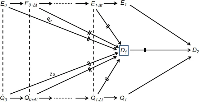
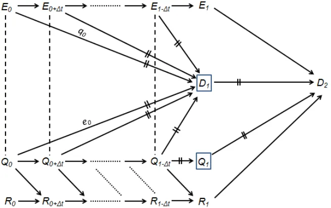
Fig. 10 depicts the situation. Q is a cause of D, though not a confounder, and E and Q modify each other’s effects on D (denoted by a lower case letter above the modified arrow to indicate dependency on the modifier’s value).
Following conditioning on D1, a new association is created between E and Q at each time point (denoted by a dash line). As a result, we observe an infinite number of open induced paths that contribute to the conditional association between E1 and D2 – for example, E1E0--Q0Q1D2.
That unwanted contribution is called colliding bias.
Fig. 11 shows the obvious solution. Conditioning on Q1 will block the induced paths and remove colliding bias. Again, the variable on which we condition is not a confounder.
One last problem still remains: there may be open induced paths through intermediaries between Q and D, such as R (Fig. 12). We have to condition on intermediary variables between the modifier and the disease (Fig. 13), just as we had to condition on intermediary variables between the confounder and the disease (Fig. 7). Again, the variable on which we condition, R1, coincides with the exposure, E1, and is not a confounder (Fig. 13).
Fig. 10. An infinite number of open induced paths following conditioning on D1
Fig. 12. An infinite number of open induced paths due to R-variables
Fig. 13. Blocking the induced paths by conditioning on R1
7. SUMMARY
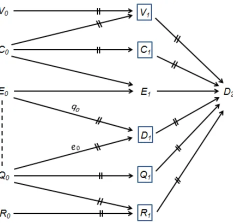
Fig. 14 summarizes the five types of variables on which we should condition to remove confounding bias, and some consequential colliding bias. To remove confounding bias, we should condition on three types of variables: two kinds of intermediaries on causal paths from the confounder to D2 (C1, V1); and disease status (D1). Since conditioning on D1 may result in colliding bias, we should also condition on two
kinds of intermediaries on causal paths from a modifier to D2 (Q1, R1).
8. DISCUSSION
Fig. 14. Five types of variables for conditioning
An obvious counter-argument takes the following form: Even if the building blocks of causal reality are time point variables, many variables do not change over time. It makes no difference, for instance, whether we condition on C1 or on C0, or on any Ct. They are essentially the same variable.
We offer the following answers:
First, in contemporary practice, many variables are clearly time dependent: smoking, drinking, weight, drug use, mental states, and so on. In those cases, conditioning on a variable at one time point is not always equivalent to conditioning on a variable at a different time point.
Second, in an indeterministic universe no variable is endowed with guaranteed stability over time. Those who think otherwise should recall our genes, time-stable variables a century ago, which turned into not-so-stable variables with contemporary gene therapy, and might become classic time-varying variables in another century. Sound methodology, on the other hand, provides for time-stable reasoning.
Third, methodological arguments prescribe a logical course of action and should not be mixed with practical considerations. In practice, we never condition on the variables that are shown in Figs. 1-14. We always
condition on an imputed version of the variable of interest (e.g., CIMPUTED) – the variable that exists in our computer when we run the analysis software [4]. That variable might differ from the variable of interest and from any variable along the measurement process.
Furthermore, which variable is replaced by CIMPUTED is a matter of interpretation, because valid substitution requires only some form of association between the variable of interest and its substitute [4]. For instance, CIMPUTED may substitute for C0 when the latterwas measured, because the two are associated through a causal path (C0CMEASUREDCIMPUTED). But it is equally valid to say that CIMPUTED substitutes for C1 – even if C0 was measured – because CIMPUTED and C1 are associated through an open path (C1C0CMEASUREDCIMPUTED). In both cases the imputed variable provides information on the values of a variable of interest. Information bias aside, it does not matter which causal structure accounts for the association between the variable of interest and its substitute. Moreover, if the effect of C0 on C1 is so strong that the two variables practically take the same value, then CIMPUTED would be a good imputation for C1 when C0 was measured. In this sense C is sometimes called a “time-stable” variable (even though its value is not inherently fixed over time).
should be considered when removing confounding bias. The conclusion that was reached here stands in sharp contrast to what is widely assumed. Of course, a different conclusion may be reached on the basis of a different axiomatization of causality, provided that coherent axioms are explicitly stated. It is crucial, however, to keep in mind the sharp distinction between an axiom of causality [3] and a definition of causality [7]: the former makes a bold claim about the way causality works; the latter trivially replaces some long phrase with a short phrase [8]. Axioms are essential for logical inference; definitions are not.
CONSENT
It is not applicable.
ETHICAL APPROVAL
It is not applicable.
COMPETING INTERESTS
Authors have declared that no competing interests exist.
REFERENCES
1. Williamson EJ, Aitken Z, Lawrie J, Dharmage SC, Burgess JA, Forbes AB.
Introduction to causal diagrams for confounder selection. Respirology 2014; 19:303-11.
2. Popper KR. The open universe: an argument for indeterminism. London, Routledge; 1988.
3. Shahar E, Shahar DJ. Marginal structural models: Much ado about (almost) nothing. Journal of Evaluation in Clinical Practice. 2013;19:214-22
4. Shahar E, Shahar DJ. Causal diagrams, information bias, and thought bias. Pragmatic and Observational Research. 2010;1:33-47.
5. Shahar E, Shahar DJ. More on selection bias. Epidemiology. 2010;21:429-30. 6. Shahar E, Shahar DJ. Causal diagrams
and three pairs of biases. In: Epidemiology – Current Perspectives on Research and Practice (Lunet N, Editor). 2012;31-62. Available:http://www.intechopen.com/book s/epidemiology-current-perspectives-on-research-and-practice
7. Hernan MA. A definition of causal effect for epidemiological research. Journal of Epidemiology and Community Health. 2004;58:265‐271.
8. Popper KR. The open society and its enemies. Princeton, Princeton University Press. 1971;2.
© 2015 Shahar and Shahar; This is an Open Access article distributed under the terms of the Creative Commons Attribution License (http://creativecommons.org/licenses/by/4.0), which permits unrestricted use, distribution, and reproduction in any medium, provided the original work is properly cited.
Peer-review history: