Benjamin Edward Krikler1,∗, Olivier Davignon1, Lukasz Kreczko1, Jacob Linacre2,
Emmanuel OlatunjiOlaiya2, andTaiSakuma1 1University of Bristol
2Rutherford Appleton Laboratory
Abstract.Binned data frames are a generalisation of multi-dimensional his-tograms, represented in a tabular format with one category per row containing the labels, bin contents, uncertainties and so on. Pandas is an industry-standard tool, which provides a data frame implementation complete with routines for data frame manipultion, persistency, visualisation, and easy access to “big data” scientific libraries and machine learning tools. FAST (the Faster Analysis Soft-ware Taskforce) has developed a generic approach for typical binned HEP anal-yses, driving the summary of ROOT Trees to multiple binned DataFrames with a yaml-based analysis description. Using Continuous Integration to run sub-sets of the analysis, we can monitor and test changes to the analysis itself, and deploy documentation automatically. This report describes this approach using examples from a public CMS tutorial and details the benefit over traditional methods.
1 Introduction
The Faster Analysis Software Taskforce (FAST) was set up in May 2017. As a group of parti-cle physicists, the initial goal was to investigate ways to address the growing data processing requirements from current and future HEP projects (e.g. at HL-LHC) against a back-drop of decelerating increases in processing power technology, similar to the HEP Software Founda-tion, whose community white paper was published around the same time [1].
FAST’s objectives include: establishing a set of best practices for analysis tooling; sharing these as feedback to developers and helping to educate peers and other users; and to contribute to existing tools or, where felt necessary, develop our own to close gaps in the HEP analysis software ecosystem. To meet these goals, FAST has met for regular hacking workshops to experiment with new ideas and techniques.
This paper describes one of our primary focuses so far, namely how an analysis whose result is produced by comparison of binned distributions can adapt to using the Pandas li-brary’s data frame implementation for internal persistency and manipulation. Such analyses are common within CMS and other experiments [2]. In this paper, analysis refers to the final stages of data processing, after event reconstruction.
This paper documents the prototype approach we have developed. Updates and devel-opments will be announced via our homepage: http://fast-hep.web.cern.ch/fast-hep/public/. Since CHEP2018, many of the packages that grew out of this prototype have now been doc-umented and added to PyPI, which can be found via the homepage.
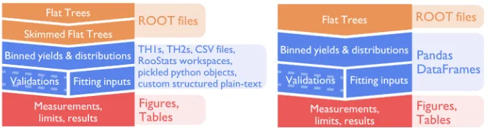
Figure 1: Overviews of a typical CMS analysis (Left) versus the approach proposed here (Right). The FAST approach is more streamlined and exploits the versatility, performance, and functionality provided by the Pandas data analysis package.
2 The FAST approach
Fig. 1 compares a typical structure for analysis code with the FAST approach.
Input files in most HEP analyses will have a ROOT-based format [3]. It is commonplace to pre-process these input files to reduce their size, either by removing events that will defi-nitely fail a later selection (a “skim”) or by removing variables that are not of use (a “slim”). Since the processing time in a typical analysis chain can be slow, this preprocessing is helpful when repeated iterations are needed as the analysis is refined to produce the final result. This is the first change in the FAST approach—remove this step completely by making sure the subsequent steps run quickly. As a result there is little-to-no need to pre-process data, making it easier to rerun as new data becomes available.
The next overall change is to simplify the internals of the analysis framework by using a single data format, the Pandas DataFrame [4], to persist data. An early step in many analyses is to produce a large numbers of ROOT histograms, where additional information will be stored in the name of the histogram in some structured way. Additional information might be persisted in other formats, such as distributions for event weighting (e.g. CSV or Python pickles), which run and event numbers to look at (e.g. JSON), how to combine the distribu-tions to fit the final result (e.g. RooStats workspaces). Pandas DataFrames are able to cover
all of these use cases, such that it is easier to manage the different data sources coherently.
Simplifying the analysis chain and homogenizing the internal data formats has two ad-ditional advantages. Firstly, it becomes easier to adapt the analysis, since their are fewer steps to consider and because the data frame approach allows the binning dimensions to be changed. Secondly, it is much easier for a newcomer to learn how to run the code, given that each internal step is more similar to the others, and because the data format can be inspected and interpreted with less knowledge of how the analysis code itself will look at it.
In order to produce the binned Pandas DataFrames, FAST has used AlphaTwirl [5], which had already been developed by Tai Sakuma, a member of FAST. AlphaTwirl is a Python-based tool which ingests event-level data and produces binned columnar data.
3 Pandas dataframes as multi-dimensional histograms
Pandas [4] is a common data-analysis toolkit written for Python, but with C++optimisations
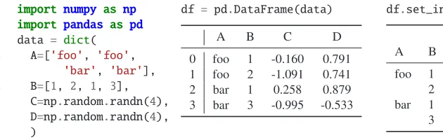
behind the scenes. The primary data format within Pandas is the DataFrame, a programmatic interface to manipulate tabular data. Within industry applications, a DataFrame is often used to represent time-series data with a fixed number of columns—similar to a ROOT TTree whose events contain only scalars and fixed-length lists. However, Pandas provides for ad-vanced labelling for its rows and columns, such as multi-indexing i.e. nested labelling. A
Listing 1: A DataFrame made from random data. Pandas makes the original row index by
using the row number. With theset_indexmethod, however, we create a DataFrame with
two data columns, indexed by two variables, which allows a DataFrame to act as a multi-dimensional histogram.
DataFrame can therefore be treated very naturally as a multi-dimensional histogram, where one row is one bin. The methods to interact with bin labelling are highly generalised, giving us the flexibility to manipulate the binned data in a consistent way regardless of the number of dimensions. Listing 1 shows an example DataFrame and how it looks once converted to a multi-index format similar to how our binned data looks.
Using Pandas in this way gives greater consistency, fewer lines of code, and direct inter-faces to other industry-standard tools, such as numpy, or machine-learning packages, such as sklearn, TensorFlow, etc.
4 Summarising ROOT trees
The first stage in the analysis pipeline is to produce the binned data frames from ROOT TTrees. To demonstrate how the FAST approach tackles this, we use the CMS HEP
tuto-rial [6], which provides real and simulated sample data sets and a set of ROOT-based C++
analysis scripts for comparisons.
4.1 The config file
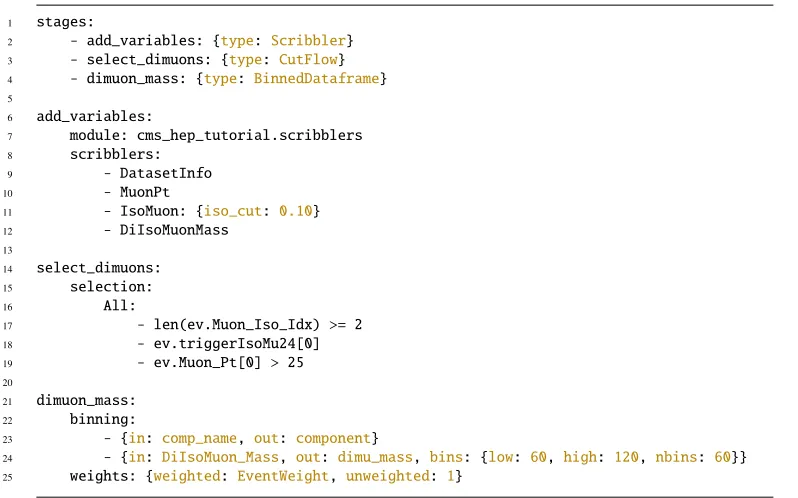
To run this step, FAST uses the AlphaTwirl package, but wraps the interface with a con-figuration file, based on YAML [7]. This concon-figuration file reduces the amount of code and isolates analysis-specific decisions and details. This, in turn, allows the code’s performance to be improved without changing the analysis itself.
An example of the configuration file is shown in Listing 2. The first section, underneath
the keystages, defines how data will be processed. There are three types of stages
avail-able at this point:CutFlows (to select events), aBinnedDataFrames (to produce summary
histograms), andScribblers (to insert variables into the event). Once the processing chain
is defined, each stage is given a complete description in the other top-level sections, whose names correspond to the stage names.
4.2 Event selection
Lines 21 to 26 of Listing 2 show how an event selection can be configured. In this example
events are selected where there are more than two isolated muons, the flagtriggerIsoMu24
is enabled, and the first muon (ordered by transverse momentum in this data) is greater than
25 GeV. These three cuts are combined with a booleanANDoperation, which is indicated by
1 stages:
2 - add_variables: {type: Scribbler}
3 - select_dimuons: {type: CutFlow}
4 - dimuon_mass: {type: BinnedDataframe}
5
6 add_variables:
7 module: cms_hep_tutorial.scribblers
8 scribblers:
9 - DatasetInfo
10 - MuonPt
11 - IsoMuon: {iso_cut: 0.10}
12 - DiIsoMuonMass
13
14 select_dimuons:
15 selection:
16 All:
17 - len(ev.Muon_Iso_Idx) >= 2
18 - ev.triggerIsoMu24[0]
19 - ev.Muon_Pt[0] > 25
20
21 dimuon_mass:
22 binning:
23 - {in: comp_name, out: component}
24 - {in: DiIsoMuon_Mass, out: dimu_mass, bins: {low: 60, high: 120, nbins: 60}}
25 weights: {weighted: EventWeight, unweighted: 1}
Listing 2: Example configuration to summarize the input ROOT trees. First we add several new variables, then we select events, and lastly we build a binned data frame.
could be replaced withAny, which would result in the cuts being combined with a boolean OR. Cuts can be nested, by putting anAnyorAlldictionary as the value of any cut.
Table 1 shows the output of this stage: a description of the number of events passing each cut for each input data set. While only unweighted counts are shown, this can be easily reconfigured to produce a weighted count. From this output, it is only a few steps to produce publication-quality reports of the cut-flow efficiencies, a common requirement in allowing results to be easily re-interpreted. In fact, the FAST approach and code has already been used to do exactly this [2].
4.3 Event distributions
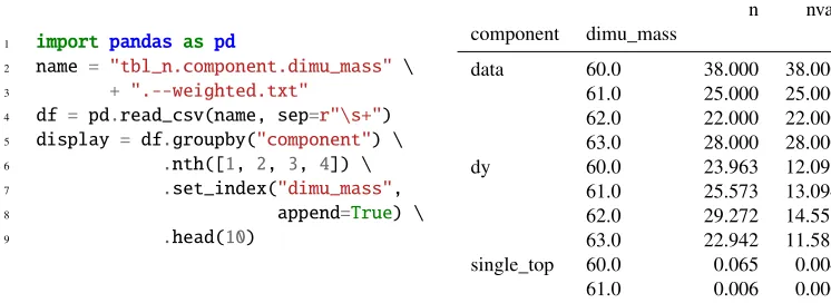
Thedimuon_massstage of the configuration in Listing 2 will produce a binned data frame containing the distribution of the dimuon mass. Only events passing the preceding event selection will be included in this stage’s output. Table 2 shows the outputs of this stage. See section 4 for how this output can be easily turned into plots.
11 - IsoMuon: {iso_cut: 0.10}
12 - DiIsoMuonMass
13
14 select_dimuons:
15 selection:
16 All:
17 - len(ev.Muon_Iso_Idx) >= 2
18 - ev.triggerIsoMu24[0]
19 - ev.Muon_Pt[0] > 25
20
21 dimuon_mass:
22 binning:
23 - {in: comp_name, out: component}
24 - {in: DiIsoMuon_Mass, out: dimu_mass, bins: {low: 60, high: 120, nbins: 60}}
25 weights: {weighted: EventWeight, unweighted: 1}
Listing 2: Example configuration to summarize the input ROOT trees. First we add several new variables, then we select events, and lastly we build a binned data frame.
could be replaced withAny, which would result in the cuts being combined with a boolean OR. Cuts can be nested, by putting anAnyorAlldictionary as the value of any cut.
Table 1 shows the output of this stage: a description of the number of events passing each cut for each input data set. While only unweighted counts are shown, this can be easily reconfigured to produce a weighted count. From this output, it is only a few steps to produce publication-quality reports of the cut-flow efficiencies, a common requirement in allowing results to be easily re-interpreted. In fact, the FAST approach and code has already been used to do exactly this [2].
4.3 Event distributions
Thedimuon_massstage of the configuration in Listing 2 will produce a binned data frame containing the distribution of the dimuon mass. Only events passing the preceding event selection will be included in this stage’s output. Table 2 shows the outputs of this stage. See section 4 for how this output can be easily turned into plots.
It can be seen how easy it is to configure such stages from the configuration file and how extra binning dimensions can be added in a generalised manner. Each binned data frame requires a list of dimensions to define how it should be binned. If a dimension is categorical, i.e. already discrete, no binning scheme is necessary; we only specify which variable to use (theinfield) and, optionally, what to call the corresponding column in the output (out). If the variable is continuous, however, a binning scheme must be provided, either as a range and the number of bins to divide this into or as a list of bin edges. Finally, a list of variables to use as events weights can also be given; for each of these, a separate DataFrame will be produced.
single_top 1 LambdaStr ev: len(ev.Muon_Iso_Idx)>=2 111 5684
LambdaStr ev: ev.triggerIsoMu24[0] 111 111
LambdaStr ev: ev.Muon_Pt[0]>25 110 111 ttbar 1 LambdaStr ev: len(ev.Muon_Iso_Idx)>=2 226 36941
Table 1: The first 10 rows of the DataFrame produced by theselect_dimuons stage in Listing 2.
4.4 New variables and custom processing steps
Custom-made stages can also be included, such as ones which calculate new variables, as shown in lines 7 to 13 of Listing 2. This allow users to write analysis-specific stages in Python, but provide key parameters from the config file.
5 Manipulating dataframes
The Pandas library allows the binned data frames from the various stages to be manipulated easily. For example, line 2 of Listing 3 shows how easy it is to add a new column to the data frame loaded in for Table 2. It next shows a more elaborate set of operations: the original “long form” data frame, where the data set is indicated in thecomponentcolumn, is converted to a “wide form” where each data set has a separate set of count and error columns. The label ordering is then changed, in order to match that from the original tutorial.
1 import pandas as pd
2 name = "tbl_n.component.dimu_mass" \ 3 + ".--weighted.txt"
4 df = pd.read_csv(name, sep=r"\s+") 5 display = df.groupby("component") \ 6 .nth([1, 2, 3, 4]) \
7 .set_index("dimu_mass",
8 append=True) \
9 .head(10)
n nvar
component dimu_mass
data 60.0 38.000 38.000
61.0 25.000 25.000
62.0 22.000 22.000
63.0 28.000 28.000
dy 60.0 23.963 12.091
61.0 25.573 13.094
62.0 29.272 14.551
63.0 22.942 11.585
single_top 60.0 0.065 0.004
61.0 0.006 0.000
10 # Convert variance --> error 11 df["err"] = np.sqrt(df.nvar) 12
13 # Switch to long-form
14 df2 = df.pivot_table(
15 index="dimu_mass",
16 columns="component",
17 values=["n", "err"])
18 df2 = df2.sort_index(axis=1,
19 ascending=False)
20
21 # Sort components to match tutorial 22 order = ["data", "ttbar", "wjets", 23 "dy", "ww", "wz", "zz", 24 "qcd", "single_top"]
25 df2 = df2.reindex(order, axis=1,
26 level="component")
n err
component data ttbar dy data ttbar dy dimu_mass
-inf 993.00 11.39 655.57 31.51 1.75 31.90 60.0 38.00 0.84 23.96 6.16 0.49 3.48 61.0 25.00 0.32 25.57 5.00 0.28 3.62 62.0 22.00 0.27 29.27 4.69 0.27 3.81 63.0 28.00 0.00 22.94 5.29 0.00 3.40 64.0 29.00 0.85 20.53 5.39 0.49 3.17 65.0 17.00 0.35 29.46 4.12 0.28 3.85 66.0 37.00 0.57 27.86 6.08 0.40 3.73 67.0 34.00 0.82 34.17 5.83 0.48 4.15 68.0 31.00 0.75 26.97 5.57 0.44 3.64 69.0 39.00 0.00 32.57 6.24 0.00 4.09 70.0 35.00 0.58 34.23 5.92 0.41 4.19 71.0 41.00 0.29 40.59 6.40 0.29 4.49
Listing 3: Left: Python code (continuing from Table 2) to convert data frame to long-form and re-order the columns, and Right: the resulting data frame.
5.1 Making plots
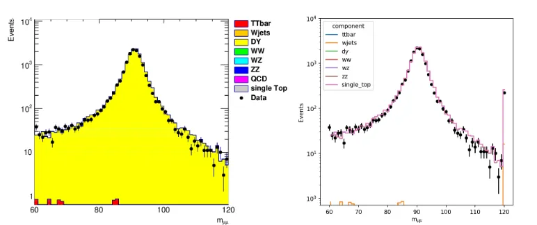
Pandas has built in support for plotting which can convert the binned data frames to figures that would be familiar to most particle physicists. Listing 4 continues from Listing 3 and demonstrates the code used to reproduce the dimuon mass distribution, and the resulting plot is shown in Fig. 2. Compared to the version produced using the CMS HEP example’s ROOT-based code, the Pandas DataFrame approach shows the same contents, although the overflow bin is shown by default, unlike ROOT. Whilst the aesthetics of the plot are different, one can reproduce the ROOT style with only an additional few lines, if really wanted.
5.2 Running a fit from binned dataframes
It is very common in the final stages of such an analysis to fit predictions to the observed data in order to extract the parameters of interest. FAST has also worked on how Pandas DataFrames can be plugged into existing tools, particularly in the case of the CMS exper-iment. Using another YAML-based config file containing details of the fit parameters and systematics, the data frames from the steps described above are converted to the necessary inputs to perform such a fit.
27 import matplotlib.pyplot as plt 28
29 data = df2.xs("data", level=1, axis=1).reset_index()
30 sims = df2.drop("data", axis=1, level=1).n
31
32 ax = plt.subplot(111)
33 sims.plot.line(linestyle="steps-mid", stacked=True, ax=ax, zorder=-1, logy=True)
34 data.plot.scatter(x="dimu_mass", y="n", yerr="err", color="k", label="data", ax=ax) 35
36 plt.ylim([0.7, 1e4]); plt.xlabel(r"m$_{\mu\mu}$"); plt.ylabel("Events"); plt.legend()
20
21 # Sort components to match tutorial 22 order = ["data", "ttbar", "wjets", 23 "dy", "ww", "wz", "zz", 24 "qcd", "single_top"] 25 df2 = df2.reindex(order, axis=1, 26 level="component")
65.0 17.00 0.35 29.46 4.12 0.28 3.85
66.0 37.00 0.57 27.86 6.08 0.40 3.73
67.0 34.00 0.82 34.17 5.83 0.48 4.15
68.0 31.00 0.75 26.97 5.57 0.44 3.64
69.0 39.00 0.00 32.57 6.24 0.00 4.09
70.0 35.00 0.58 34.23 5.92 0.41 4.19
71.0 41.00 0.29 40.59 6.40 0.29 4.49
Listing 3: Left: Python code (continuing from Table 2) to convert data frame to long-form and re-order the columns, and Right: the resulting data frame.
5.1 Making plots
Pandas has built in support for plotting which can convert the binned data frames to figures that would be familiar to most particle physicists. Listing 4 continues from Listing 3 and demonstrates the code used to reproduce the dimuon mass distribution, and the resulting plot is shown in Fig. 2. Compared to the version produced using the CMS HEP example’s ROOT-based code, the Pandas DataFrame approach shows the same contents, although the overflow
bin is shown by default, unlike ROOT. Whilst the aesthetics of the plot are different, one can
reproduce the ROOT style with only an additional few lines, if really wanted.
5.2 Running a fit from binned dataframes
It is very common in the final stages of such an analysis to fit predictions to the observed data in order to extract the parameters of interest. FAST has also worked on how Pandas DataFrames can be plugged into existing tools, particularly in the case of the CMS exper-iment. Using another YAML-based config file containing details of the fit parameters and systematics, the data frames from the steps described above are converted to the necessary inputs to perform such a fit.
27 import matplotlib.pyplot as plt 28
29 data = df2.xs("data", level=1, axis=1).reset_index() 30 sims = df2.drop("data", axis=1, level=1).n
31
32 ax = plt.subplot(111)
33 sims.plot.line(linestyle="steps-mid", stacked=True, ax=ax, zorder=-1, logy=True) 34 data.plot.scatter(x="dimu_mass", y="n", yerr="err", color="k", label="data", ax=ax) 35
36 plt.ylim([0.7, 1e4]); plt.xlabel(r"m$_{\mu\mu}$"); plt.ylabel("Events"); plt.legend()
Listing 4: Continuing from Listing 3, we build the plot shown in the right of Fig. 2 from the wide form data frame.
Figure 2: The dimuon mass distribution in data and from the predicted simulated events, Left: The plot produced using the HEP tutorial’s code using ROOT, and Right: The equivalent plot using the FAST approach.
6 Continuous integration for analysis
Continuous Integration (CI) has become a mainstay of any modern development environ-ment. In addition to using modern tools within the analysis, FAST checks the analysis using CI. The pipeline currently used to test FAST code runs: static code checks and style compli-ance, unit tests, integrations tests, and automated documentation generation when the master branch is updated. The static code checks ensure that the code remains at a high quality (i.e. PEP8 using Flake8 [8]). Unit tests (written with Pytest [9]) run individual functions and classes through specific checks to pinpoint when an interface has unexpectedly changed, and catch common bugs early. Integration tests, on the other hand, run the whole chain of the analysis on a small testing sample of the data, and compare the outputs for each stage against what is expected. The tools to run these steps were written by FAST, and allows a gen-eral overview of when an analysis has changed and by how much. Future versions will also check the analysis’ computing performance such as time per event, memory requirements, etc. Finally, the last stage in the CI pipeline generates documentation (using Sphinx [10]), such as examples and a cross-linked API reference, which can be deployed automatically.
Overall, using CI significantly reduces the effort to maintain a consistent, functioning, and
documented analysis chain.
7 Comparisons to traditional approaches
There are many differences between the analysis approach described here compared to a more
to help produce new variables and plot the distributions. Future versions of the FAST code-base will improve the ability to plot binned data frames by adding general functions to assist this, further simplifying the code needed for each analysis. By comparison, the equivalent code in the CMS public analysis (which can be found in the tar-ball in [6]), implemented in C++and using ROOT, contains more than 600 lines of code. Whilst it is hard to make an “apples to apples” comparison between a Python-based tool and an analysis code written in C++, this nevertheless demonstrates how the FAST approach is able to compress analysis decisions into fewer lines of code, whilst retaining the expressiveness needed to be generic.
Another key metric for comparison is the speed of execution. Here the C++-based anal-ysis code performs better than the current implementation of the FAST approach, taking roughly 4 seconds to execute compared to the FAST code’s 60 seconds. Whilst this is a big difference in performance, the fact that this analysis is controlled through the configura-tion file allows the code to be optimised behind the scenes. AlphaTwirl uses a Python-based event-loop, and preliminary studies suggest that adapting this to a chunked and vectorised alternative using uproot [11], can achieve around factor 30 increases in run-times, i.e. equiv-alent or better than the C++example.
8 Conclusion
The FAST approach has the goals of building a more modular, flexible, and concise way to run a binned particle physics analysis. The generic configuration files that describe each step make it easier to reproduce and share a given analysis, as well as providing a separation between code and analysis details. In addition they allow the underlying code to be optimised behind-the-scenes. Using Pandas DataFrames as the sole means to transfer data between the various analysis stages reduces the complexity and helps adapt the data for use in other industry-standard tools such as Jupyter notebooks.
Although what has been presented here is being used on the CMS experiment already, FAST intends to bring this approach to maturity by modularising the code-base further to provide a series of PyPI-served packages. In addition, the overall performance is being improved, in particular to make use of the packages coming from the scikit-HEP project, including uproot and awkward-array.
References
[1] A.A. Alves, Jr et al. (2017),1712.06982
[2] CMS Collaboration, Journal of High Energy Physics2018, 25 (2018)
[3] I. Antcheva, M. Ballintijn, B. Bellenot et al., Comp. Phys. Comm.180, 2499 (2009) [4] W. McKinney,Data Structures for Statistical Computing in Python, inProceedings of
the 9th Python in Science Conference(2010), pp. 51 – 56
[5] T. Sakuma,AlphaTwirl: A Python library for summarizing event data into multivariate categorical data, inCHEP 2018(2019),1905.06609
[6] CMS HEP Tutorial, http://opendata.cern.ch/record/50 and http://ippog.org/resources/ 2012/cms-hep-tutorial, accessed: 2018-10-04
[7] Yaml website, http://yaml.org/, accessed: 2018-10-04
[8] Flake8 website, https://gitlab.com/pycqa/flake8, accessed: 2019-07-03
[9] H. Krekel et al.,pytest 3.10(2004),https://github.com/pytest-dev/pytest
[10] Sphinx website,http://sphinx-doc.org/, accessed: 2019-07-03