QCD@Work 2018
The Light CP-Even Higgs Boson Mass of the MSSM at
Three-Loop Accuracy
Edilson A.Reyes Rojas1,∗and A. RaffaeleFazio1,∗∗
1Departamento de Fisica, UNAL, Bogotá, Colombia
Abstract.In this paper we are going to discuss the relevant aspects related to the calculation of the higher order corrections to the lightest CP-even Higgs bo-son mass of the minimal supersymmetric standard model with real parameters (rMSSM). We have computed these corrections using the Feynman diagram-matic approach with a precision of three-loop in the SUSYQCD sector. The renormalization scheme adopted in this work is based on a variant of dimen-sional regularization where the so called dimendimen-sional reduction is performed in order to preserve supersymmetry to all perturbative orders. The calculation will extend the region of validity of previous studies to the whole parameters space. The emerging loop integrals have been computed by exploiting new pro-posed approaches based on the dispersion relation techniques for the numerical calculation of three-loop vacuum integrals with arbitrary mass scales.
1 Introduction
The analysis of the scale dependent properties of the Higgs sector in the Standard Model (SM) and beyond the SM scenarios (BSM) have been discussed by several authors for the last decade. The currently accepted analysis in the SM was presented in a completely way up to two-loop order in the references [1] and [2]. In these works the triviality, the vacuum stability problem and the hierarchy problem were studied by assuming that no new physics appears up to the Planck scale (ΛP) and therefore by assuming an unnatural amount of fine-tuning
(1034) for the squared Higgs boson mass at the electroweak (EW) scale. In this approach the
near-criticality of the Higgs quartic coupling (λ) and its beta-function is used as a guideline to go beyond the SM. However, there are strong physical arguments to believe that the SM is an effective field theory valid in a limited energy range belowΛP. These include the dark matter
observations, the baryon asymmetry in the universe, the neutrino oscillations, the Yukawa hierarchies in flavour physics, etc. If one insists that the naturalness argument is valid and would represent a real problem of the theory, then one has to conclude that physics beyond the SM has to appear at the TeV scale in the next runs of the LHC or in the coming experi-ments at future colliders like the ILC. One way to test that is through the comparison between the experimental observations and the theoretical predictions in order to confirm whether the Higgs boson is actually the predicted particle by the SM or is part of an extended model. Any deviation of the experimental results from the SM predictions would suppose a signal of new physics beyond the SM.
QCD@Work 2018
The most popular BSM scenario that may describe these new phenomena is formulated as a supersymmetric extension of the SM, the minimal supersymmetric standard model (MSSM). The MSSM can provide for a solution to the fine-tuning and the hierarchy problem by the existence of new bosonic degrees of freedom that cancel the loop contributions with the un-wanted quadratic divergences. Moreover, similar contributions render the effective potential
stable, thus the MSSM simultaneously cures the vacuum stability problem. In most of the benchmark scenarios of the MSSM the Higgs boson found at LHC corresponds to the light-est CP-even Higgs boson with a massMhwhich is not a free input parameter but a prediction
coming from the parameters of the theory. The upper bound on its predicted mass at leading order (LO) is given by the Z gauge boson mass, MZ = 91.2 GeV, leading to the exclusion
of the MSSM at current collider experiments. However, higher order quantum corrections to the MSSM Higgs boson mass lead to a considerably large shift in the upper limit towards
Mh ≤135 GeV. Additionally, the expected experimental uncertainty associated to the Higgs
boson mass is of the order of 100-200 MeV at the LHC [3] and this value could go even down at the future ILC reaching a roughly value of 50 MeV [4]. At two-loop order the theoretical uncertainty has been estimated to 3-5 GeV [5] and as a consequence, it is mandatory to per-form calculations at next-to-next-to-next to leading order (NNNLO) to reduce the theoretical uncertainty to the same order as the experimental accuracy expected at the LHC and ILC colliders. Our goal in this article is take you through the details of the computation of the radiative corrections toMhin the rMSSM at this level of accuracy.
2 Radiative Corrections to
M
hin the MSSM
The Higgs sector of the MSSM have five physical Higgs bosons, three of them are neutral, the others two are charged. In lowest order these are the lightest (h) and heavy (H) CP-even Higgs bosons, the CP-odd Higgs boson (A), and the two charged Higgs bosons (H±). At tree level, the Higgs sector can be parametrized in terms of the gauge boson masses (MWandMZ),
the mass of the CP-odd Higgs boson (MA) andtanβ = v2/v1, which is the ratio of the two
vacuum expectation values. The masses of the five Higgs boson particles follow as predic-tions. For the MSSM the status of higher-order corrections to the masses and mixing angles in the neutral Higgs sector is quite advanced and widely studied due to radiative corrections can give large contributions to the values of these parameters. Regarding the corrections to the lightest Higgs boson mass the state of the art is as follows. At one-loop level the full corrections are found in reference [6] with real parameters. The detailed results of a Feyn-man diagrammatic (FD) calculation of the leading two-loop QCD corrections at order O(ααs)
can be found in [7], in particular the O(αbαs) [8] and O(αtαs) [9] contributions using the FD
approach are known in the limit where the external momentum vanishes and in the MSSM version with complex parameters. In this limit there is an alternative procedure to compute the above corrections, the Effective Potential (EP) approach. The analytical expressions for
the two-loop leading-log neutral Higgs boson masses using the MSSM effective potential can
be found in [10] and the references therein. A comparison of the corresponding two-loop results in the FD and EP approaches of the mass of the lightest CP-even Higgs boson in the MSSM at O(ααs) can be found in [11]. The FD approach has the advantage that it can allow
for non-vanishing external momentum, in contrast to the EP method where all contributions are evaluated at zero external momentum. An evaluation of the momentum dependence of the two-loop corrections, including all the terms involving the QCD couplings, in the modi-fied dimensional reduction scheme (DR) was presented in [12]. The renormalization scheme
QCD@Work 2018
A0 T3 U4 U5 U6
Figure 1:Basis of three-loop vacuum integrals obtained from the IBP reduction with Reduze.
space. This regularization procedure is performed in order to preserve supersymmetry to all perturbative orders. The latest status of the momentum-dependent two-loop corrections was discusses recently in [15, 16] using a hybrid on-shell-DRscheme, whereMAand the tadpoles
are renormalized on-shell, whereas the Higgs boson fields andtanβare renormalizedDRand including corrections ofO(p2α
tαs).
3 Higgs Boson Mass at Three-loop Accuracy
In this section we are going to discuss our diagrammatic computation of the corrections toMh
at three-loop accuracy. We restrict the calculation to the supersymmetric quantum chromo-dynamics (SUSYQCD) sector where the Higgs couples to the top quark or its super-partner. In the perturbative expansion of the Higgs mass, these are the terms of orderα2sαt, whereαs
is the square of the strong coupling constant andαtdenotes the coupling of the Higgs to the
top quark. This is not the first computation ofMhat this order, there is already the
diagram-matic computation performed by Harlander et al. [17], whereMhwas computed at O(αtα2s).
Their results were expressed in terms ofDRparameters for the quark and squark masses and implemented in the computer program H3m for Mathematica. However, the contributions obtained in this work have exploited the methods of asymptotic expansion in order to pro-vide precise approximations in some relevant mass hierarchies. We have gone beyond these approximations and therefore we have avoided perform asymptotic expansions at the integral level in order to obtain a general expression valid for any election of the input masses. Taking in mind the above statement we have organized our computation as follows. The three-loop radiative correction toMhis obtained by evaluating the neutral Higgs boson
self-energies () and the tadpoles (T) for the fieldsh,HandAaccording with the equation
ˆ
(3)
hh =
(3)
hh −Re
(3)
AA sαsβ+cαcβ
2 −
e
2sWMW
Th(3) √
2C1+
T(3)H √
2C2
, (1)
where the letter sigma with a hat represents the three-loop renormalized correction to Mh,
whileandT are three-loop unrenormalized quantities evaluated at zero external momen-tum. The coefficientsC1 andC2are functions of the mixing anglesαandβwhich are
re-sponsible for the diagonalization of the bilinear part of the Higgs potential. All the necessary Feynman diagrams and their corresponding amplitudes are generated with FeynArts [18]. In total there are 7738 self-energies and 7180 tadpoles to be evaluated. The generated ampli-tudes with FeynArts are not regularized. With the help of the Mathematica package FeynCalc [19] we have written a routine that implements the regularization of Feynman integrals by di-mensional reduction. Thus, we performed the Dirac and Lorentz algebra over numerators of the integrals in the Q4S space. It is worth to mention that the Q4S algebra for diagrams which contain the cubic vertex quark-squark-gluino requires a special treatment. This vertex introduces theγ5matrix in the Dirac traces. We have dealtγ5as an anti-commuting object,
which is allowed in our computation because traces with an odd number ofγ5always contain
QCD@Work 2018
0 500 1000 1500 2000
123 124 125 126 127 128 129 130
Μr Mh
GeV
Ge
V
(a)At=1500 GeV
tanβ=10
2000 1000 0 1000 2000 100
105 110 115 120 125 130
At Mh
GeV
Ge
V
(b)µr=200 GeV
tanβ=10
0 10 20 30 40
120 122 124 126 128 130
tanΒ
Mh GeV
(c)At=1500 GeV
µr=250 GeV
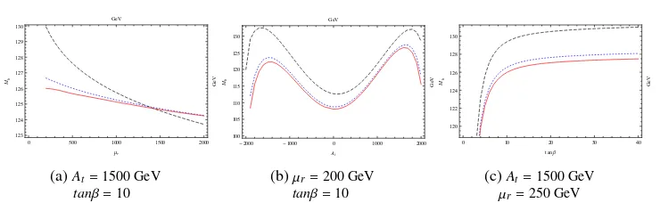
Figure 2:Dependence ofMhon (a)µr; (b)Atand (c)tanβ. Black dashed and blue dotted lines are the
one- and two-loop predictions of FeynHiggs. The red solid line depicts our three-loop predictions.
algebra of numerators, each amplitude can be expressed as a superposition of a set of scalar integrals which can contain irreducible numerators. We have classified and listed all different
scalar integrals that we need in our calculation, in total there are 3525 scalar integrals that we must evaluate. This set of scalar integrals are not independent of each other but related by the integration by parts (IBP) and Lorentz invariance (LI) identities. We have used the IBPs to generate a homogeneous system of linear equations where the scalar integrals are the unknowns. The system can be reduced to a small set of irreducible integrals, the so called Master Integrals. This is something that cannot be done by hand, because there are thou-sand of equations. Thus, we have used the program Reduze [20], an implementation of the Laporta algorithm, in order to reduce the set of scalar integrals to a superposition of a small set of master integrals. We have found the basis of six master integrals depicted in Figure 1, where each topology can contain at most four different mass scales. The functions A0 and T3
have very well known analytical solutions for any configuration of masses, while the three-loop functions U4, U5 and U6 have an analytical solution just for the cases where there are one or two independent mass scales but when there are three or four independent scales a numerical evaluation of the three-loop vacuum integrals is required.
The analysis of convergence and the numerical evaluation of the integrals which are unknown analytically was performed with the help of the program TVID developed by A. Freitas [21]. TVID uses the discontinuities coming from the one-loop self-energy and the one-loop ver-tex in four dimensions to produce dispersion relations that are useful in the evaluation of the three-loop vacuum integrals in terms of one- and two-dimensional integral representa-tions. In all cases we have been able to get analytical expressions for the divergent part of the master integrals while the finite part could be numerically evaluated with up to 10 digits of accuracy. It is possible to reach this precision because the numerical integrations are at most 2-dimensional and therefore there is a controlled treatment of any singularities. It is also necessary an additional sub-renormalization procedure due to the presence of non-local divergences in the unrenormalized Higgs self-energies as well as in the Higgs tadpoles. As a consequence, we have to include also diagrams with counter-term insertions in order to remove sub-divergences. At three-loop level we need the renormalization of the gluino mass, the squark masses, the stop mixing angle and the top quark mass at the one-loop order. In addition we need the two-loop counterterms for the stop mixing angle, the stop quark masses and the top quark mass. The necessary expressions for these counterterms can be consulted in the review [22] and references therein.
Once the UV divergences and sub-divergences are renormalized we get a finite correction to
Mh. Using this contribution we have studied the dependence of the Higgs boson massMh
on the renormalization scaleµr (Fig. 2a), the soft-breaking parameterAt (Fig. 2b) and the
input parametertanβ(Fig. 2c). In Figure 2 we show these dependences for a benchmark
QCD@Work 2018
0 500 1000 1500 2000
123 124 125 126 127 128 129 130 Μr Mh GeV Ge V
(a)At=1500 GeV
tanβ=10
2000 1000 0 1000 2000 100 105 110 115 120 125 130 At Mh GeV Ge V
(b)µr=200 GeV
tanβ=10
0 10 20 30 40
120 122 124 126 128 130 tanΒ
Mh GeV
(c)At=1500 GeV
µr=250 GeV
Figure 2:Dependence ofMhon (a)µr; (b)Atand (c)tanβ. Black dashed and blue dotted lines are the
one- and two-loop predictions of FeynHiggs. The red solid line depicts our three-loop predictions.
algebra of numerators, each amplitude can be expressed as a superposition of a set of scalar integrals which can contain irreducible numerators. We have classified and listed all different
scalar integrals that we need in our calculation, in total there are 3525 scalar integrals that we must evaluate. This set of scalar integrals are not independent of each other but related by the integration by parts (IBP) and Lorentz invariance (LI) identities. We have used the IBPs to generate a homogeneous system of linear equations where the scalar integrals are the unknowns. The system can be reduced to a small set of irreducible integrals, the so called Master Integrals. This is something that cannot be done by hand, because there are thou-sand of equations. Thus, we have used the program Reduze [20], an implementation of the Laporta algorithm, in order to reduce the set of scalar integrals to a superposition of a small set of master integrals. We have found the basis of six master integrals depicted in Figure 1, where each topology can contain at most four different mass scales. The functions A0 and T3
have very well known analytical solutions for any configuration of masses, while the three-loop functions U4, U5 and U6 have an analytical solution just for the cases where there are one or two independent mass scales but when there are three or four independent scales a numerical evaluation of the three-loop vacuum integrals is required.
The analysis of convergence and the numerical evaluation of the integrals which are unknown analytically was performed with the help of the program TVID developed by A. Freitas [21]. TVID uses the discontinuities coming from the one-loop self-energy and the one-loop ver-tex in four dimensions to produce dispersion relations that are useful in the evaluation of the three-loop vacuum integrals in terms of one- and two-dimensional integral representa-tions. In all cases we have been able to get analytical expressions for the divergent part of the master integrals while the finite part could be numerically evaluated with up to 10 digits of accuracy. It is possible to reach this precision because the numerical integrations are at most 2-dimensional and therefore there is a controlled treatment of any singularities. It is also necessary an additional sub-renormalization procedure due to the presence of non-local divergences in the unrenormalized Higgs self-energies as well as in the Higgs tadpoles. As a consequence, we have to include also diagrams with counter-term insertions in order to remove sub-divergences. At three-loop level we need the renormalization of the gluino mass, the squark masses, the stop mixing angle and the top quark mass at the one-loop order. In addition we need the two-loop counterterms for the stop mixing angle, the stop quark masses and the top quark mass. The necessary expressions for these counterterms can be consulted in the review [22] and references therein.
Once the UV divergences and sub-divergences are renormalized we get a finite correction to
Mh. Using this contribution we have studied the dependence of the Higgs boson mass Mh
on the renormalization scaleµr (Fig. 2a), the soft-breaking parameterAt (Fig. 2b) and the
input parametertanβ(Fig. 2c). In Figure 2 we show these dependences for a benchmark
scenario where all the squark masses, except the stop mass, have the same value defined to
be MS US Y = 1000 GeV, while we have chosen a value of Mg˜ = 1500 GeV for the gluino
mass andMt=173.3 GeV for the top quark mass. To generate the MSSM Higgs predictions
at one and two -loop level we have used the code FeynHiggs [23]. These contributions are represented in the plots of Fig. 2 with the black dashed and blue dotted curves, respectively. Besides, the red solid line represents our three-loop prediction. The three-loop corrections are quite sizeable, amounting a size of about 1 TeV and with negative sign for our election of input parameters. It leads to a more stable dependence ofMhwith the renormalization scale
µrand have a strong dependence ontanβfor small values close totanβ=5, while for large
values abovetanβ=20 the variation ofMhis marginal.
4 Conclusion
Following the Feynman diagrammatic procedure described in the above section, we have obtained a finite expression for the renormalized three-loop correction to the lightest Higgs boson mass. Taking in mind that nowadays in the MSSM is no clear at priori what the hierarchies of the masses will turn out to be, we have avoided the application of asymptotic expansions and we have obtained the correction in terms of a set of three-loop master integrals whose numerical evaluation is possible thanks to the dispersion relation techniques for any arbitrary mass hierarchy. A complete phenomenological analysis of our numerical results will be presented in future works.
Acknowledgements. This work is partially financially supported by the research grant N. 34729, Minimal Supersymmetric Standard Model Higgs Boson Masses to High Accu-racy of the callCONVOCATORIA NACIONAL DE PROYECTOS PARA EL FORTALECIMIENTO DE LA INVESTIGACIÓN, CREACIÓN E INNOVACIÓN DE LA UNIVERSIDAD NACIONAL DE COLOMBIA 2016-2018.
References
[1] Buttazzo D., Degrassi G., Giardino P.P., Giudice G., Sala F., Salvio A. and Strumia, A., JHEP,1312, 089 (2013). [2] B. A. Kniehl, A. F. Pikelner and O. L. Veretin, Nucl. Phys. B896, 19 (2015).
[3] CERN Report No. CERN-LHCC-2006-021; CMS-TDR- 008-2, (2006), http://cmsdoc.cern.ch/cms/cpt/tdr/.
[4] J. A. Aguilar-Saavedra et al. [ECFA/DESY LC Physics Working Group] (2001) [arXiv:hep-ph/0106315].
[5] B. C. Allanach, A. Djouadi, J. L. Kneur, W. Porod and P. Slavich, JHEP0409, 044 (2004). [6] A. Dabelstein, Nucl. Phys. B456, 25 (1995).
[7] S. Heinemeyer, W. Hollik and G. Weiglein, Eur. Phys. J. C9, 343 (1999).
[8] S. Heinemeyer, W. Hollik, H. Rzehak and G. Weiglein, Eur. Phys. J. C39, 465 (2005). [9] S. Heinemeyer, W. Hollik, H. Rzehak, G. Weiglein, Phys. Lett. B652, 300 (2007). [10] M. Carena, M. Quiros and C. Wagner, Nucl. Phys. B461, 407 (1996).
[11] M. Carena, H. Haber, S. Heinemeyer, W. Hollik, C. Wagner, and G. Weiglein, Phys. B580, 29 (2000). [12] S. Martin, Phys. Rev. D71, 016012 (2005).
[13] I. Jack et al., Phys. Rev. D50, 5481 (1994). W. Siegel, Phys. Lett. B84, 193 (1979). [14] D. Stockinger, JHEP0503, 076 (2005).
[15] S. Borowka, T. Hahn, S. Heinemeyer, G. Heinrich and W. Hollik, Eur. Phys. J. C74, 8, 2994 (2014). [16] G. Degrassi, S. Di Vita and P. Slavich, Eur. Phys. J. C75, 2, 61 (2015).
[17] R. Harlander, P. Kant, L. Mihaila and M. Steinhauser, JHEP1008, 104 (2010). [18] T. Hahn, Comput. Phys. Commun.140, 418 (2001).
[19] V. Shtabovenko, R. Mertig, F. Orellana, Comput. Phys. Commun.207, 432 (2016). [20] C. Studerus, Comput. Phys. Commun.181, 1293 (2010).
[21] A. Freitas, JHEP1611, 145 (2016) [arXiv:1609.09159 [hep-ph]]. [22] L. Mihaila, Adv. High Energy Phys.2013, 607807 (2013).