ANALYSIS OF RADIATION CHARACTERISTICS OF A PROBE-EXCITED RECTANGULAR RING ANTENNA BY THE DYADIC GREEN’S FUNCTION APPROACH S. Lamultree, C. Phongcharoenpanich, S. Kosulvit
and M. Krairiksh Faculty of Engineering
King Mongkut’s Institute of Technology Ladkrabang Bangkok 10520, Thailand
Abstract—Radiation characteristics of a probe-excited rectangular ring antenna are investigated by using the dyadic Green’s function approach. The radiation characteristics, such as radiation pattern, beam-peak direction, half-power beamwidth and directivity, are analyzed. For the specified operating frequency, the ring width and ring height are selected as the same cross-sectional dimension of rectangular waveguide operated at the dominant mode. The effects of the excited probe and rectangular ring to the modal distributions are described. For the desired modal distribution, the directivity primarily depends on the ring lengths. For compact size of the proposed antenna, the ring length of 0.4λis chosen to provide a bidirectional pattern with the calculated half-power beamwidth in E-plane and H-plane of 100 and 69 degrees respectively, and directivity of 4.43 dBi. Furthermore, the prototype antenna was fabricated and measured. The coincided results between the theory and the experiment are obtained.
1. INTRODUCTION
been extensively conducted as reviewed in literature [6–11]. From the aforementioned researches, it is evident that development of a bidirectional antenna that has suitable characteristics for a particular application is desired. Moreover, the low cost must be considered since the number of cell is very large. The bidirectional antennas using a linear probe excited circular ring was proposed [12–14] to serve these demands. Although the circular ring provides the slightly higher gain than the rectangular ring, its beamwidth cannot be easily adjusted due to the symmetrical structure. The rectangular ring antenna is very attractive to adjust the beamwidth following the applications by changing the ring width and ring height. Furthermore, the desired directivity is easily obtained by varying the ring length. This paper presents the radiation characteristic investigations of a bidirectional antenna using a probe-excited rectangular ring. The analysis includes the equivalent electric and magnetic current densities. In addition, the position of an excited probe that involves the modal distribution is comprised. Theoretically, there are many techniques to analyze the radiation from the aperture fed by probe in open literature [15– 23]. Each method possesses its advantages and disadvantages. In this paper, the dyadic Green’s function approach [22–30] is used to analyze the radiation characteristics of the proposed antenna since it is straightforward, and the closed form with physical insight is obtained. The rigorous analysis is expressed in detail.
This paper is organized as follows. Section 2presents the theory of the antenna including the antenna structure and the derivation expressions. In Section 3, the normalized magnitude of the equivalent electric and magnetic current densities for various modal distributions are shown. The radiation characteristics as the function of antenna parameters are studied. Then, the antenna fabrication and measurement are performed. The experimental results are illustrated in Section 4. Finally, the conclusions are presented in Section 5.
2. THEORY
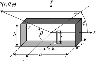
The proposed antenna consists of a linear electric probe of length l
aligned along y direction at the position (x = s, y = −b/2, z = 0). The probe is surrounded by rectangular ring of width a, height b and lengthc, respectively. There are two apertures at the planesz= +c/2 and z=−c/2respectively, as shown in Fig. 1.
s P(r,θ,φ)
c b
l
z
y
x
r φ
θ
a Figure 1. Antenna structure.
direction is assumed. In addition, the time convention e−jωt is used and suppressed, where ω = 2πf and f is the frequency. The scalar wave function solved by the method of separation of variables is [24]
ψe±z
omn(kz) =
Cx Cy Sx Sy
e∓jkzz, m= 1,2,3, . . .
n= 0,1,2, . . . (1)
where
Sx = sin
kx
x+a
2
, Cx = cos
kx
x+ a
2
,
Sy = sin
ky
y+b 2
, Cy = cos
ky
y+b 2
,
kx = mπ
a , ky = nπ
b , kc =k 2
x+ky2, kz =
k2−(k2 x+k2y), k=ω√µ0ε0, µ0 = 4π×10−7H/m, ε0 = 8.854×10⁻¹²F/m.
The superscript ±z denotes the field radiations in +z and −z
directions, respectively. The subscript e and o are an abbreviation for the even and odd functions, respectively.
The vector wave functions, Memn and Nomn, satisfy the vector
Dirichlet boundary condition at the conducting wall (an×Memn= 0
and an×Nomn = 0), wherean is the normal unit vector. The vector
wave functions Memn and Nomn represent the electric field of TEmn
and TMmn modes, respectively. In the same manner, Momn and Nemn are the vector wave functions that satisfy the vector Neumann
boundary condition an ×
∇ ×Momn
∇ ×Nemn
= 0. Hence, they can be
written as
Me
omn(kz) =∇ × azψeomn(kz)
and
Ne
omn(kz) =
1
k∇ × ∇ × azψeomn(kz)
. (3)
Following the method of magnetic dyadic Green’s function and applying the Ohm-Rayleigh method, the magnetic dyadic Green’s function due to an electric source (GHJ(R, R)) that satisfies the dyadic differential equation is
∇ × ∇ ×GHJ
R, R−k2GHJ
R, R=∇ × IδR−R. (4)
δR−R denotes the Dirac delta function, which is equal to
δ(x−x)δ(y−y)δ(z−z) in the Cartesian coordinate. I is the unit dyadic. The primed variables (x, y, z) and unprimed variables (x, y, z) are the source point and the observation point, respectively. The relationship in (4) is defined in the domain −a2 ≤ x ≤ a2,
−b
2 ≤y ≤ b
2,−∞ ≤z≤ ∞, and the Neumann boundary condition
an× ∇ ×GHJR, R= 0, (5)
atx=−a/2anda/2,y=−b/2andb/2. The eigenfunction expansion ofGHJ in term of the rectangular vector wave functions is given by [24]
GHJ
R, R = ∞
−∞
dkz jk ab
m,n
(2−δ0)κ πabk2
c (κ2−k2)
Nemn(kz)Memn(−kz)
+Momn(kz)Nomn(−kz)
(6)
where, κ2 =mπa 2+nπb 2+kz2 =k2c +kz2,δ0 denotes the Kronecker
delta function defined as
δ0=
1 m orn= 0
0 m and n= 0 (7)
By applying the contour integration, (6) becomes
G±HJz R, R=
−jk ab
m, n
2−δ0 k2
ckz
Nemn(+kz)Memn(−kz)
+Momn(+kz)Nomn(−kz)
; z > z
+jk
ab
m, n
2−δ0 k2
ckz
Nemn(−kz)Memn(+kz)
+Momn(−kz)Nomn(+kz)
; z < z.
The electric dyadic Green’s function due to an electric source
GEJ(R, R) is obtained from the relationship
∇ ×GHJ
R, R=IδR−R+k2GEJ
R, R. (9)
Then, we obtain
G±EJzR, R=−azaz 1 k2δ
R−R
+
−j
ab
∞
m=1
∞
n=0
2−δ0 k2
ckz
Memn(+kz)Memn(−kz)
+Nomn(+kz)Nomn(−kz)
; z > z
+j
ab
∞
m=1
∞
n=0
2−δ0 k2
ckz
Memn(−kz)Memn(+kz)
+Nomn(−kz)Nomn(+kz)
; z < z,
(10)
M±emnz (kz) = (−axkyCxSy+aykxSxCy)e∓jkzz, (11)
N±omnz (kz) =
1
κ(∓axjkzkxCxSy∓ayjkzkySxCy
+azkc2SxSye∓jkzz, (12)
M±omnz (kz) = (axkySxCy−aykxCxSy)e∓jkzz (13)
and
N±emnz (kz) =
1
k
±axjkzkxSxCy±ayjkzkyCxSy+azk2cCxCy
e∓jkzz.
(14)
The electric fieldERinside the ring with the probe excitation is determined by using
E±zR=∓jωµ0
V
G±EJR, R·JRdV, (15)
where G±EJ(R, R) is obtained from (10) and J(R) is the electric current distribution along the probe. In this paper, the linear probe directed in y direction has a small diameter compared to the wavelength and the sinusoidal distribution is reasonably assumed as
JR =ayIm d sink
l−y−b
2
whereImis the maximum current that is normalized to be unity andd
is the diameter of the probe. Since the probe is oriented inydirection, hence onlyGxyEJ,GyyEJ, andGzyEJ can contribute to the electric field. All of these components are derived and shown as
Gxy,EJ±z =
− j ab ∞ m=1 ∞ n=0
2−δ0 k2
ckz
−kxkyCxSySxC
+ 1
κ2k 2
zkxkyCxSySxCy
e−jkz(z−z); z > z
j ab ∞ m=1 ∞ n=0
2−δ0 k2
ckz
−kxkyCxSySxCy
+ 1
κ2k 2
zkxkyCxSySxCy
e+jkz(z−z); z < z,
(17)
Gyy,EJ±z =
− j ab ∞ m=1 ∞ n=0
2−δ0 k2
ckz
k2xSxCySxCy
+ 1
κ2k 2
zky2SxCySxCy
e−jkz(z−z); z > z
j ab ∞ m=1 ∞ n=0
2−δ0 k2
ckz
kx2SxCySxCy
+ 1
κ2k 2
zky2SxCySxCy
e+jkz(z−z); z < z
(18)
and
Gzy,EJ±z=
− j ab ∞ m=1 ∞ n=0
2−δ0 k2
ckz j κ2k
2
ckzkySxSySxCye−jkz(z−z
)
;
z > z j ab ∞ m=1 ∞ n=0
2−δ0 k2 ckz − j κ2
k2ckzkySxSySxCye+jkz(z
−z)
;
z < z.
(19)
Consequently, the electric field in x,y, andz components are
Ex±z = −ωµ0Im
abd ∞ m=1 ∞ n=0
2−δ0 k2
ckz
(−k) sin
kx
s+a
2
×
cos(kyl)−cos(kl)
k2 y −k2
−kxky+k
2 zkxky κ2 ×cos kx x+a
2 sin ky y+b
2
e−jkzz
Ey±z = −ωµ0Im abd ∞ m=1 ∞ n=0
2−δ0 k2
ckz
(−k) sin
kx
s+a
2
×
cos(kyl)−cos(kl) k2
y −k2
kx2+k
2 zk2y κ2 ×sin kx x+a
2 cos ky y+b
2
e−jkzz
(21)
and
Ez±z = −jωµ0Im abd ∞ m=1 ∞ n=0
2−δ0
κ2 (−k) sin
kx
s+a 2
×
cos(kyl)−cos(kl) k2
y −k2
kysin
kx
x+a
2 ×sin ky y+b
2
e−jkzz
. (22)
The equivalent magnetic current densities (Ms) at the two apertures
are obtained from
M±szR= E±zR
z=±c/2×(±az) (23)
The resultant equivalent magnetic current densities are
M±szR = −ωµ0Im
abd ∞ m=1 ∞ n=0
2−δ0 k2
ckz
(−k) sin
kx
s+a
2
×
cos(kyl)−cos(kl) k2
y −k2
e−jkzz
±ax
kx2+k
2 zk2y κ2 ×sin kx x+a
2 cos ky y+b
2
∓ay
−kxky+k
2 zkxky
κ2 ×cos kx x+a
2 sin ky y+ b
2
. (24)
By following the same fashion, the magnetic field HR can be found from
HR=
V
GHJ
where GHJ, after some mathematical manipulations, can be derived
as
Gxy,HJ±z = k
ab ∞ m=1 ∞ n=0
(2−δ0) k2
cκ
SxCySxC
× kx2+k2y
e−jkz(z−z); z > z
−k2 x−k2y
e+jkz(z−z); z < z, (26)
Gyy,HJ±z = 0 (27)
and
Gzy,HJ±z =
−jk ab ∞ m=1 ∞ n=0
(2−δ0) k2
ckzκ
kc2kxCxSySxSye−jkz(z−z
)
; z > z
jk ab ∞ m=1 ∞ n=0
(2−δ0)
k2 ckzκ
k2ckxCxSySxSye+jkz(z−z); z < z.
(28)
The magnetic field components are
Hx±z = ±kIm
abd ∞ m=1 ∞ n=0
(2−δ0) κk2
c
(−k) sin
kx
s+a
2
×
cos(kyl)−cos(kl)
k2
y−k2
e−jkzzk2
x+ky2
×sin
kx
x+a
2 cos ky y+b
2
, (29)
Hy±z = 0 (30)
and
Hz±z = ∓jkIm abd ∞ m=1 ∞ n=0
(2−δ0) κk2
c
(−k) sin
kx
s+a
2
×
cos(kyl)−cos(kl)
k2
y −k2
e−jkzz
×kxk2c kz
cos
kx
x+a
2 cos ky y+b
2
. (31)
Similarly, the equivalent electric current densitiesJs
are
and
J±szR = kIm
abd
∞
m=1
∞
n=0
2−δ0 k2
cκ
(−k) sin
kx
s+a
2
×
cos(kyl)−cos(kl) k2
y −k2
kx2+ky2e−jkzz
×
±aysin
kx
x+ a
2
cos
ky
y+ b
2
.(33)
After the equivalent magnetic and electric current densities are readily obtained, the far-zone radiated field from a probe-excited rectangular ring antenna can be subsequently found by using radiation parameters from [31]. By neglecting mutual coupling and reflection at the edge of the ring and assuming that there is no reflection from the opposite aperture, a superposition of the fields from the two apertures can be applied. The fields radiated from the two apertures are combined with the same phase but in opposite directions. The resultant field can be written as follows
Eθ±z(r, θ, φ) −jke
−jk(r∓c
2cosθ)
4πr
L±φz+ηNθ±z
, (34)
Eφ±z(r, θ, φ) +jke
−jk(r∓c2cosθ) 4πr
L±θz−ηNφ±z
(35)
and
|ET otal(r, θ, φ)| =
Eθ+z(r, θ, φ) +Eθ−z(r, θ, φ)2
+
Eφ+z(r, θ, φ) +Eφ−z(r, θ, φ)
21/2
, (36)
where
Nθ±z = ±kIm
abd
∞
m=1
∞
n=0
2−δ0 k2
cκ ab
4j (−k) sin
kx
s+ a 2
×
cos (kyl)−cos (kl) k2
y−k2
e−jkzz±k2
x+k2y
cosθsinφ
Nφ±z = ±kIm abd ∞ m=1 ∞ n=0
2−δ0 k2
cκ ab
4j(−k) sin
kx
s+a 2
×
cos (kyl)−cos (kl) k2
y−k2
e−jkzz±k2
x+ky2
cosφ
×SA−SA SB+SB, (38)
L±θz = −ωµ0Im
abd ∞ m=1 ∞ n=0
2−δ0 k2
ckg ab
4j(−k) sin
kx
s+ a 2
×
cos (kyl)−cos (kl) k2
y−k2
e−jkzz
±
kx2+k
2 zky2 κ2
cosθcosφ
×SA−SA SB+SB∓
−kxky + k2
zkxky κ2
×cosθsinφSA+SA SB−SB (39)
and
L±φz = −ωµ0Im
abd ∞ m=1 ∞ n=0
2−δ0 k2
ckg ab
4j (−k)
×sin
kx
s+a
2
cos (kyl)−cos (kl) k2
y−k2
e−jkzz
×
∓
kx2+k
2 zk2y κ2
sinφSA−SA SB+SB
∓
−kxky+ kz2kxky
κ2
cosφSA+SA SB−SB.(40)
where
SA = sin [(a/2 ) (ksinθcosφ+kx)]
a/2 (ksinθcosφ+kx) e
jkxa/2,
SA = sin [(a/2 ) (ksinθcosφ−kx)]
a/2 (ksinθcosφ−kx)
e−jkxa/2,
SB = sin [(b/2 ) (ksinθsinφ+ky)]
b/2 (ksinθsinφ+ky)
ejkyb/2
and SB = sin [(b/2 ) (ksinθsinφ−ky)]
b/2 (ksinθsinφ−ky)
e−jkyb/2.
3. RADIATION CHARACTERISTICS
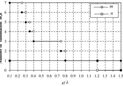
The total electric field is obtained from the summation of electric field distribution of a probe excited rectangular ring antenna as written in (20)–(22), (29)–(31) and (36). It should be pointed that considering the minimum number of summation terms of m and n, that provide efficiently accurate results for minimizing the running time of the computed results, is important. Therefore, the appropriate number ofm andnfor the numerical convergence should be obtained. Fig. 2shows the number of summation m and n for various c. The criterion of convergence consideration is that the deviation of half-power beamwidth of the antenna is less than 0.5 degree. Apparently, the number of summationmandnshould be larger (m= 7 andn= 1) for the shorterc, due to the influence of the higher order modes. The number of summationmandnwill be decreased to 1 and 0 respectively, for the larger c because the higher order modes are reduced rapidly. For the dominant mode (m = 1 and n= 0) the magnitude of current densities keeps almost constant (see Fig. 3). Thus, it is obvious that
m= 7 andn= 1 will be used for all ring lengths. These values are used to obtain the characteristics of the antenna that are explicitly expressed hereafter. From the total fields of the antenna as shown in (36), it is obvious that the radiation characteristics of the antenna depend on the following parameters, i.e., probe position (s), probe length (l), ring width (a), ring height (b) and ring length (c). In this paper, the initial probe length is 0.25λfor the reason of good impedance matching. Since the cross-section of the antenna is the same as a rectangular waveguide, in this circumstance the ring width and ring height are chosen to be the dimension of a standard waveguide operating at the dominant mode.
0 1 2 3 4 5 6 7
0.1 0.2 0.3 0.4 0.5 0.6 0.7 0.8 0.9 1.0 1.1 1.2 1.3 1.4 1.5
c/λ
Number of
summation
m,
n
m n
TE10
TE11
TE30
TE31
TM11
TM31
Normalized maximum magnitude
|
M
s
/
M
s
-T
E10
|
0 0.001 0.010 0.100 1.000
probe position ring length in +z direction (zs/λ)
0 0.050.10 0.150.200.25 0.300.350.40 0.450.50 0.550.600.650.70 0.75
probe position ring length in +z direction (zs/λ)
0 0.050.10 0.150.200.25 0.300.350.40 0.45 0.50 0.550.60 0.650.70 0.75
TE10
TE11
TE30
TE31
TM11
TM31
0
/
NNormalized maximum magnitude
|
η
Js
Ms
-T
E10
|
0.001 0.010 0.100 1.000
(a)
(b)
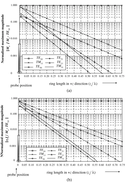
Figure 3. Normalized magnitude of Ms and ηJs for various aperture
distanceszs (where probe is located at (x=s= 0,y=−b/2,z= 0)):
(a)Ms, (b)ηJs.
Thus, the ring width of a, and ring height of b = a/R are selected, where R is the ratio of a/b and R ≥ 1; in this paper R = 2is used. The cut-off wavelength is obtained from [32]
λc = 2π
mπ a
2
+
nπ
b
Thus, a choice of TE10 mode is restricted in the range of λ2 < a < λ.
It is noted that a should be far away from the upper range to avoid higher modes. Thenceforth,a= 0.70λandb= 0.35λare selected, and these values are fixed throughout this paper. Accordingly, the antenna characteristics depend on the ring length.
Following (20)–(22) and (29)–(31), the equivalent current densities of the antenna are determined. It is revealed that a short ring length contains several modes in the vicinity of the probe and the evanescent waves of the higher order modes near the probe still have a considerable level at the aperture as shown in Fig. 3. Furthermore, the TE10 mode
keeps the constant value for any zs (where zs is the distance of c/2
away from the probe position), whereas the higher order modes are lower as the further distance to the aperture. They reduce rapidly whenzs= 0.75λ. In addition, it is found that some modes do not exist
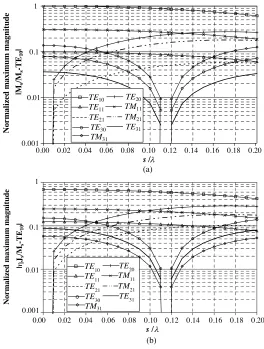
especially the modes with even m, that is different from those in the rectangular waveguide. However, the modes with evenm are induced and strengthen when probe is shifted from the center (x = s = 0,
y = −b/2, z = 0) whereas modes with odd m are decreased as shown in Fig. 4. The dominant mode TE10 is still stronger than the
others. It should be noted that modal distribution inside a probe-excited rectangular ring antenna also has strong effect to the input impedance of the proposed antenna that is left for further study.
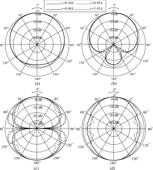
According to (34)–(40) in Section 2, the electric fields are plotted. Fig. 5 shows the radiation pattern of the antenna as a function of c. The radiation pattern of a single aperture in +z and −z directions at
zs = ±c/2is shown for the condition of the field that only radiates
toward +z and −z directions and there is no coupling between the apertures. Then, radiation pattern from two apertures is displayed from the combination of a single aperture in +z and −z directions. It should be noted that the dummy load is terminated at the aperture of
−z and +z directions for considering radiation pattern radiated from the aperture of +z and −z directions, respectively. The bidirectional pattern can be produced. It is observed that for the c shorter than 0.1λ, the radiated field is same as the pattern of a dipole antenna, viz., the E-plane pattern (φ = 90◦) approaches figure of eight and almost omnidirectional pattern in H-plane (φ= 0◦). Moreover, by increasing
c, the pattern in E-plane is wider and then split. Then it becomes a bidirectional pattern with side lobes. The H-plane pattern has wider beam for the shorter c because the aperture separation affects the radiation patterns. In addition, theE-plane pattern has null and the
directions to form bidirectional pattern.
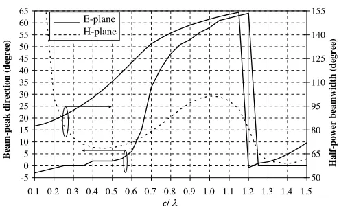
In addition, the beam-peak direction of E-plane will be slightly tilted from z axis (θ = 0◦ and θ = 180◦) due to the influence of asymmetrical probe position at the upper and lower side (i.e., it is located at the lower side) as shown in Fig. 6. It is found that a bidirectional pattern is obtained at c ≤ 0.6λ and will occur again with existed side lobe atc≥1.25λ(for the beam peak directs +5 and
−5 degrees tilted fromz axis). Furthermore, in Fig. 6, the half-power beamwidth in the E-plane and the H-plane have the opposite curve, viz., a wider beamwidth and a narrower beamwidth inE-plane andH
-0.001 0.01 0.1
1
0.00 0.02 0.04 0.06 0.08 0.10 0.12 0.14 0.16 0.18 0.20 s /λ
Normal
ized
m
aximum magnitude
|M
s
/M
s
-TE
10
|
TE10 TE11
TE21
TE30
TM31 TE20 TM11
TM21 TE31
0.001 0.01 0.1 1
0.00 0.02 0.04 0.06 0.08 0.10 0.12 0.14 0.16 0.18 0.20 s /λ
Normalized maximum magn
it
ude
|
η
Js
/M
s
-T
E10
|
TE10 TE11 TE21 TE30 TM31
TE20 TM11 TM21 TE31
(a)
(b)
Figure 4. Normalized magnitude of Ms and ηJs for variouss(where
plane respectively, as the longer ring length except atc≥1.3λ. These result to the directivity of the antenna that will be then described. Note that the narrow beamwidth is required for the high directivity.
The directivity is a figure of merit that quantifies the antenna directive properties comparing with an isotropic antenna. The maximum directivity is defined as the maximum radiation intensity of that antenna (Umax) over the radiation intensity of isotropic radiator (Prad/4π). The high radiation intensity with the low radiated power is required to enhance directivity. The maximum radiation intensity is obtained from combining of the maximum amplitude of electric field
60 90 30 0 30 60 90 120 150 180 150 120 -30 dB -20 dB -10 dB 0 dB θ (c) (d) 60 90 0 0 30 60 90 120 150 180 150 120 -30 dB -20 dB -10 dB 0 dB θ 60 90 30 0 30 60 90 120 150 180 150 120 -30 dB -20 dB -10 dB 0 dB θ 60 90 30 0 30 60 90 120 150 180 150 120 -30 dB -20 dB -10 dB 0 dB θ
c=0.10λ
c=0.40λ
c=0.95λ
c=1.45λ
(a) (b) o o o o o o o o o o o o o o o o o o o o o o o o o o o o o o o o o o o o o o o o o o o o o o o o
-5 0 5 10 15 20 25 30 35 40 45 50 55 60 65
0.1 0.2 0.3 0.4 0.5 0.6 0.7 0.8 0.9 1.0 1.1 1.2 1.3 1.4 1.5 c/λ
Beam-peak direction (degree)
50 65 80 95 110 125 140 155
Half-power beamwidth (degree)
E-plane H-plane
Figure 6. Beam-peak direction and half-power beamwidth for various ring lengths.
that radiates from +zand −z apertures as
E2 =|Eθ,+z+Eθ,−z|2+|Eφ,+z+Eφ,−z|2
=
|Eθ,+z|2+|Eθ,−z|2+ 2|Eθ,+z| |Eθ,−z|cos (ξθ,+z−ξθ,−z)
+
|Eφ,+z|2+|Eφ,−z|2+2|Eφ,+z||Eφ,−z|cos (ξφ,+z−ξφ,−z)
.(42)
The optimum ring length that provides the maximum directivity must be clarified. Fig. 7 shows the maximum directivity as a function of ring length when l= 0.25λ, a= 0.70λand b= 0.35λ. In Fig. 7(a), it can be seen that the maximum radiation intensity can be found at θ = 0◦ and φ = 90◦ by combining the square of magnitude of electric field aperture at +z (|Eθ,+z|2) and −z directions (|Eθ,−z|2)
respectively, with the term of phase difference (ξ+z −ξ−z) between
+zand−zapertures, as defined by subscript +zand−z, respectively. Equation (42) shows thatEφhas null in this direction. Therefore, only a component ofEθ is shown in Fig. 7(a). The term of phase difference
the narrower beamwidth with existed side lobe. However, for the bidirectional pattern with no side lobe, the appropriated ring length of 0.4λ provides the directivity of 4.43 dBi. For the compact size of antenna, the ring length of 0.4λis chosen.
0.1 0.3 0.4 0.5 0.6 0.7 0.8 0.9 1.0 1.1 1.2 1.3 1.4 1.5
|E
|
2 (V/m
)
2
c/λ
9
3.5 10×
9
3.0 10×
9
2.5 10×
9
2.0 10×
9
1.5 10×
9
1.0 10×
8
5.0 10×
8
0.5 10
− ×
9
1.0 10
− ×
0
|Eθ, +z|2
|Eθ, -z|2
2|Eθ, +z||Eθ, -z|cos(ξθ.+z)cos(ξσ.+z)
|E|2
c/λ
Dire
ct
iv
it
y
(dBi
)
Prad (W)&
Umax
(W/steradian)
Directivity
Prad
Umax
0.0 0.5 1.0
1.5 2.0 2.5 3.0 3.5 4.0 4.5 5.0
0.0
10
1.6 10×
10
1.4 10×
10
1.2 10×
10
1.0 10×
9
0.8 10×
9
0.6 10×
9
0.4 10×
9
0.2 10×
0.1 0.2 0.3 0.4 0.5 0.6 0.7 0.8 0.9 1.0 1.1 1.2 1.3 1.4 1.5
(a)
(b)
0.2
Figure 7. Directivity, radiated power and radiation intensity for various ring lengths: (a) Magnitude of radiated field. (b) Directivity,
4. EXPERIMENTS
To verify the calculated results by using the dyadic Green’s function approach, the numerical results from Method of Moments (MoM) with the Rao-Wilton-Glisson (RWG) basis functions [33] and measured results are compared. It is noted that using RWG-MoM, the mutual coupling and reflection from the edges of ring is taken into account. However, the computation time for RWG-MoM is results, 4.47 times longer than that from the dyadic Green’s function approach. One reason is that the closed form is not available for RWG-MoM. For the experiment, a prototype antenna was fabricated with the designed parameters as pointed in the previous section to operate at the operating frequency of 1.9 GHz. The ring was made of brass of 1 mm thickness with the dimension of the ring height equals 5.5 cm and the ring width equals 11.0 cm. The ring length is 6.3 cm. This structure was excited by a linear electric probe made of copper rod with the diameter of 2mm. The probe length was 4.3 cm and was located at (x=s= 0.4 cm,y=−b/2,z= 0) for impedance matching. This probe was connected to a transmission line via an N type connector. The photograph of the fabricated antenna is shown in Fig. 8. The radiation patterns of the antenna were measured by using an HP8720C Network Analyzer.
Figure 8. Photograph of the prototype antenna.
60°
90° 30°
0°
30°
60°
90°
120°
150°
180°
150° 120° -30 dB
-20 dB -10 dB 0 dB Τ
60°
90° 30°
0°
30°
60°
90°
120°
150°
180°
150° 120° -30 dB
-20 dB -10 dB 0 dB Τ MoM with RWG
Dyadic Green's function
Measurement
Figure 9. Measured and calculated results of radiation pattern for
c= 0.4λ: (a)E-plane, (b) H-plane.
-30 -25 -20 -15 -10 -5 0
0.90 0.92 0.94 0.96 0.98 1.00 1.02 1.04 1.06 1.08 1.11
f/fo
|S11
|
(dB)
Figure 10. Measured|S11|of the antenna.
from dyadic Green’s function approach compared with the measured half-power beamwidth in E-plane and H-plane of 90 and 67 degrees respectively. The simulation from RWG-MoM provides half-power beamwidth inE-plane andH-plane of 106 and 70 degrees, respectively. Furthermore, it is found that at (θ= 0◦, φ= 90◦) the gains of 4.43 dBi, 4.72dBi and 4.40 dBi are yielded from the dyadic Green’s function approach, RWG-MoM and measurement, respectively.
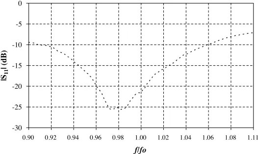
It should be noted that the impedance characteristic is not aimed in this paper; however, the|S11|of the antenna was measured to clarify the matching condition as shown in Fig. 10. It is found that |S11|
is −21.5 dB (lower than −10 dB) at the operating frequency. The measured bandwidth (|S11|<−10 dB) and gain are 16% and 4.40 dBi,
respectively.
5. CONCLUSIONS
This paper presents the investigations of a bidirectional antenna using a probe-excited rectangular ring by using the dyadic Green’s function approach. The antenna characteristics depend on the probe length, ring width, ring height and ring length. In addition, the bidirectional patterns without side lobes are obtained for the appropriated ring lengthcfrom 0.10λto 0.65λ. The side lobe is occurred whenc≥1.25λ. Furthermore, the beam-peak direction in E-plane is slightly tilted from z-axis because the probe position is not symmetry between the upper and lower sides of the ring. For H-plane pattern, the beam directs in +z and −z directions for any ring length of interest because of the symmetrical geometry in its plane. For the specified cross-sectional dimensions, the ring length is selected to achieve the optimum radiation pattern. Furthermore, the experiment was set up to verify the theoretical predictions. Apparently, the measured radiation pattern coincided with the calculated result except at around
θ = 90◦ due to the edge effect. The computed directivity of 4.43 dBi and measured gain of 4.40 dBi are obtained. The polarization of this antenna at the directions along the street cell (+zand−zdirections) is linear because there is only one component of electric field. Although the sinusoidal current distributions, disregarded mutual coupling and omitted reflection at the edge of the ring is assumed, the experimental results provide the validity of the theoretical predictions.
ACKNOWLEDGMENT
REFERENCES
1. Huang, C.-W. P., A. Z. Elsherbeni, J. J. Chen, and C. E. Smith, “FDTD characterization of meander line antennas for RF and wireless communications,”Progress In Electromagnetics Research, PIER 24, 185–199, 1999.
2. Wang, Y. J. and C. K. Lee, “Design of dual-frequency microstrip patch antennas and application for IMT-2000 mobile handsets,”
Progress In Electromagnetics Research, PIER 36, 265–278, 2002. 3. Eldek, A. A., A. Z. Elsherbeni, and C. E. Smith,
“Dual-wideband square slot antenna with a U-shaped printed tuning stub for personal wireless communication systems,” Progress In Electromagnetics Research, PIER 53, 319–333, 2005.
4. Song, Y., Y.-C. Jiao, G. Zhao, and F.-S. Zhang, “Multiband CPW-FED triangle-shaped monopole antenna for wireless applications,” Progress In Electromagnetics Research, PIER 70, 329–336, 2007.
5. Si, L.-M. and X. Lv, “CPW-FED multi-band omni-directional pla-nar microstrip antenna using composite metamaterial resonators for wireless communications,” Progress In Electromagnetics Re-search, PIER 83, 33–146, 2008.
6. Cho, K., T. Hori, H. Tozawa, and S. Kiya, “Bidirectional rod antennas comprising collinear antenna and parasitic elements,”
IEICE Transactions on Communications, No. 6, 1255–1260, 1998. 7. Cho, K., T. Hori, and K. Kagoshima, “Bidirectional rod antennas comprising a narrow patch and parasitic elements,” IEICE Transactions on Communications, No. 9, 2482–2489, 2001. 8. Arai, H. and K. Cho, “Cellular and PHS base station antenna
systems,” IEICE Transactions on Communications, No. 9, 980– 992, 2003.
9. Lamultree, S., C. Phongcharoenpanich, S. Kosulvit, and M. Krairiksh, “An equivalent circuit of a bidirectional antenna using a probe excited rectangular ring,” The Proceedings of the 2004 IEEE International Symposium on Antennas and
Propagation and USNC/URSI National Radio Science Meeting,
Vol. 2, 1672–1675, 2004.
10. Lamultree, S., C. Phongcharoenpanich, S. Kosulvit, and M. Krairiksh, “Investigations of a bidirectional antenna using a probe excited rectangular ring,” The Proceedings of Asia-Pacific Microwave Conference 2005, Vol. 5, 2943–2946, 2005.
application,” International Journal of Infrared and Millimeter Waves, Vol. 28, No. 1, 25–31, 2007.
12. Kosulvit, S., M. Krairiksh, C. Phongcharoenpanich, and T. Wakabayashi, “A simple and cost-effective bidirectional antenna using a probe excited circular ring,”IEICE Transactions on Electronics, Vol. E84-C, No. 4, 443–450, 2001.
13. Phongcharoenpanich, C., T. Sroysuwan, P. Wounchoum, S. Ko-sulvit, and M. Krairiksh, “An array of a probe excited circular ring radiating bidirectional pattern,”The Proceedings of the 2002 IEEE International Symposium on Antennas and Propagation and
USNC/URSI National Radio Science Meeting, Vol. 2, 292–294,
2002.
14. Kosulvit, S., M. Krairiksh, C. Phongcharoenpanich, and T. Wakabayashi, “A bidirectional antenna using a probe excited circular ring,” The Proceedings of the 2001 Progress in Electromagnetics Research Symposium, 423, 2001.
15. Risser, J. R.,Microwave Antenna Theory and Design, Mc-Graw-Hill, 1949.
16. Yaghjian, A., “Approximate formulas for the far field and gain of open-ended rectangular waveguide,” IEEE Transactions on Antennas and Propagations, Vol. 32, No. 4, 378–384, 1984. 17. Jia, H., K. Yoshitomi, and K. Yasumoto, “Rigorous analysis of
rectangular waveguide junctions by fourier transform technique,”
Progress In Electromagnetics Research, PIER 20, 263–282, 1998. 18. Jia, H., K. Yoshitomi, and K. Yasumoto, “Rigorous analysis
of E-/H-plane junctions in rectangular waveguides using fourier transform technique,” Progress In Electromagnetics Research, PIER 21, 273–292, 1999.
19. El Sabbagh, M. and K. Zaki, “Modeling of rectangular waveguide junctions containing cylindrical posts,” Progress In Electromagnetics Research, PIER 33, 299–331, 2001.
20. Li, L.-W., T.-X. Zhao, M.-S. Leong, and T.-S. Yeo, “A spatial-domain method of moments analysis of a cylindrical-rectangular chirostrip,”Progress In Electromagnetics Research, PIER 35, 165– 182, 2002.
21. Booty, M. R. and G. A. Kriegsmann, “Reflection and transmission from a thin inhomogeneous cylinder in a rectangular TE10
waveguide,” Progress In Electromagnetics Research, PIER 47, 263–296, 2004.
Microwave Theory and Techniques, Vol. 40, No. 12, 2172–2180, 1992.
23. Yao, H.-W. and K. A. Zaki, “Modeling of generalized coaxial probes in rectangular waveguides,” IEEE Transactions on Microwave Theory and Techniques, Vol. 43, No. 12, 2805–2811, 1995.
24. Tai, C. T., Dyadic Green’s Functions in Electromagnetic Theory, 2nd ed., IEEE Press, 1994.
25. Tai, C. T. “On the eigenfunction expansion of dyadic Green’s function,” The Proceedings of IEEE, Vol. 61, 480–481, 1973. 26. Moroney, D. T. and P. J. Cullen, “The Green’s function
perturbation method for solution of electromagnetic scattering problems,”Progress In Electromagnetics Research, PIER 15, 221– 252, 1997.
27. Li, L.-W., M.-S. Leong, P.-S. Kooi, T.-S. Yeo, and K. H. Tan, “An analytic representation of dyadic Green’s functions for a rectangular chirowaveguide: Part I — Theory,” IEEE Transactions on Microwave Theory and Techniques, Vol. 47, No. 1, 67–73, 1999.
28. Leong, M., K. H. Tan, L.-W. Li, P.-S. Kooi, and T.-S. Yeo, “An analytic representation of dyadic Green’s functions for a rectangular chirowaveguide: Part II — Results,” IEEE Transactions on Microwave Theory and Techniques, Vol. 47, No. 1, 74–81, 1999.
29. Liu, S., L. W. Li, M. S. Leong, and T. S. Yeo, “Rectangular conducting waveguide filled with uniaxial anisotropic media: A modal analysis and dyadic Green’s function,” Progress In Electromagnetics Research, PIER 25, 111–129, 2000.
30. Marliani, F. and A. Ciccolella, “Computationally efficient expressions of the dyadic Green’s function for rectangular enclosures,” Progress In Electromagnetics Research, PIER 31, 195–223, 2001.
31. Balanis, C. A.,Antenna Theory Analysis and Design, John Wiley & Sons, 1997.
32. Balanis, C. A., Advanced Engineering Electromagnetics, John Wiley & Sons, 1989.