SOL: Segmentation with Overlapping Labels

(1)

Western University Western University

Scholarship@Western

Electronic Thesis and Dissertation Repository

1-22-2018 10:00 AM

SOL: Segmentation with Overlapping Labels

Karin Ng

The University of Western Ontario

Supervisor Boykov, Yuri Y.

The University of Western Ontario Graduate Program in Computer Science

A thesis submitted in partial fulfillment of the requirements for the degree in Master of Science © Karin Ng 2018

Follow this and additional works at: https://ir.lib.uwo.ca/etd

Part of the Computer Sciences Commons

Recommended Citation Recommended Citation

Ng, Karin, "SOL: Segmentation with Overlapping Labels" (2018). Electronic Thesis and Dissertation Repository. 5185.

https://ir.lib.uwo.ca/etd/5185

This Dissertation/Thesis is brought to you for free and open access by Scholarship@Western. It has been accepted for inclusion in Electronic Thesis and Dissertation Repository by an authorized administrator of

(2)

Image segmentation is a fundamental problem in Computer Vision which involves seg-menting an image into two or more segments. These segments usually correspond to objects of interest in the image, i.e. liver, kidney’s etc. The classic approach to this problem segments the image into mutually exclusive segments. However, this approach is not well-suited when segmenting overlapping objects, e.g. cells, or when segmenting a single object into multiple parts that are not necessarily mutually exclusive. Moreover, we show that optimization methods for multi-part object segmentation with different priors/constraints may better avoid local minima in case of a relaxation allowing parts to overlap.

We propose a novel segmentation model, i.e. Segmentation with Overlapping Labels (SOL), which allows for the objects’ multiple parts to overlap. This aids in overcom-ing the aforementioned issue of local minima with standard optimization approaches. We prove that SOL is an NP-hard problem, as well as introduce a novel move-making optimization framework to find an approximate solution to SOL. Our qualitative and quantitative results show that our proposed method outperforms state-of-the-art algo-rithms for multi-part segmentation.

Keywords: Computer vision, image segmentation, discrete optimization, graph cuts, shape priors

(3)

Acknowlegements

This work was partially supported by NIH grants R01-EB004640, P50-CA174521, and R01-CA167632. We thank Drs. S. O’Dorisio and Y. Menda for providing the liver data (NIH grant U01-CA140206). This work was also supported by NSERC Discovery and RTI grants (Canada) for Y. Boykov and O. Veksler.

(4)

Abstract ii

Acknowledgements iii

List of Figures vi

List of Tables x

1 Introduction 1

1.1 Image Segmentation . . . 2

1.2 Binary Segmentation . . . 3

1.2.1 Energy . . . 3

1.2.2 Optimization via Graph Cuts . . . 5

1.2.3 Submodularity . . . 8

1.3 Multi-Label Segmentation . . . 8

1.3.1 Energy . . . 8

1.3.2 Optimization via

α

-Expansion . . . 9

1.3.3 Optimizable Energies via

α

-Expansion . . . 10

1.4 Second-Order Shape Priors . . . 11

1.4.1 Hedgehog Shape Prior . . . 12

1.5 Prior Work Limitations . . . 14

1.6 Thesis Contributions . . . 15

1.7 Thesis Outline . . . 15

2 SOL: Segmentation with Overlapping Labels 16 2.1 Overview and Motivation . . . 17

2.2 SOL Energy . . . 20

2.3 SOL Optimization . . . 22

2.4 Binary Optimization Moves . . . 23

2.4.1

α

-Expansion Move: . . . 24

(5)

Submodularity . . . 25

2.4.2

α

-Contraction Move: . . . 26

Submodularity . . . 28

2.5 NP-Hardness Proof . . . 29

3 Experiments 31 3.1 Synthetic Example . . . 32

3.2 Liver Segmentation . . . 34

4 Future Work and Conclusion 45

Bibliography 47

Curriculum Vitae 49

(6)

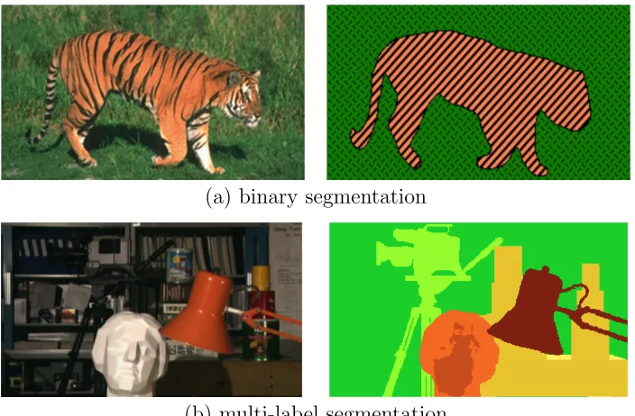
1.1 Classical image segmentation. (a) depicts a binary segmentation of a tiger from its background and (b) depicts multiple objects segmented from the background. . . 2

1.2 Example of graph-cut segmentation. From left to right: (a) base image, (b) only using the data term, (c) data and smoothness term. . . 4

1.3 An example of a graph construction and segmentation. (a) shows the graph nodes. (b) and (c) show the edges corresponding to the unary and pairwise potentials of energy (1.1), respectively. The fully constructed graph G is shown in (d). (e) shows a possible s/t-cut and the severed edges by thes/t-cut are shown in grey. (f) shows the corresponding pixel labeling of the s/t-cut in (e). . . 6

1.4 Example of a graph with a path from the source s to the sink t. . . 7

1.5 Image restoration usingα-expansion [4]. The noisy image (b) is taken in as the input, and α-expansion returns an estimated image (c) as the output. 10

1.6 (a) shows an example of a shape that is star-convex w.r.t. the centercand (b) is an example of a shape that is not star-convex. Note that in (b), the pixelq is on the line between cand p but does not lie inside the shape. . 11

1.7 Hedgehog constraints [18] for segmentS. (a) user-seed defines a signed dis-tance mapd. (b) surface normals ¯nS

p ofS are constrained by∠(¯npS,∇dp)≤θ. 12

1.8 shows how to approximate hedgehog constraint at pixel p. Cone Cθ(p) of

the allowed surface normals (blue) is enforced by ensuring that all the neighbouring pixels in the corresponding polar cone Cbθ(p) (red) lie inside

S if p∈S. . . 13 1.9 (a) synthetic example with a complex seed (red). (b) non-smooth vector

field that leads to conflicting hedgehog constraints (highlighted by the red lines). Note that due to over-constraints, no segmentation can pass through the red lines on (b) leading to (c) incorrect segmentation of [18]. 14

(7)

2.1 illustrates the negative effect of using complex seeds [18, 16]. (a) the image to be segmented and the foreground seeds (shown in red), (b) distance map of the seeds, (c) the non-smooth gradient of the distance map, and (d) segmentation result of [18]. The segmentation artifacts in (d) are due to conflicting hedgehog constraints caused by the non-smooth vector field (c). . . 17

2.2 top row shows how we split the complex seed in Fig. 2.1 into three simple ones. Middle row shows the distance map for each seed. Bottom row shows the field of gradients for the distance maps. Notice these distance maps and vector fields are smooth. . . 18

2.3 (b) shows the three different local minima found by α-expansion with the Hedgehog constraint when enforcing mutually exclusive foreground labels. Note the over-segmentation of the first expansion and under-segmentation of subsequent expansions. (d) shows the three different local minima of our proposed method (allowing foreground labels to overlap) with the Hedge-hog constraint. . . 19

2.4 depicts a possible segmentation with three foreground labels (F1, F2, F3)

and one background label B, represented by fk

p for each pixel p.

Further-more, the hatched area corresponds to the foreground segment and the dotted area corresponds to the background, represented by fp. . . 20

2.5 (a) shows a sample of a current segmentation. (b) shows a feasible ex-pansion for label F1. Notice how F1 expands while F2 and F3 remain

unaffected. . . 24

2.6 (a) shows a sample of a current segmentation. (b) shows a feasible con-traction for label F1. Notice how F1 loses pixel support while F2 and F3

remain unaffected. . . 26

2.7 (a) the hatched area shows the pixels that may change their data term in a contraction (i.e. switch from foreground to background). Pixel p is a part of this set and pixel q is not. (b) shows an example of a feasible contraction. Notice that for pixelp, the data term changed to background while pixel q remained foreground. . . 27

3.1 (a) depicts our original synthetic image while (b) displays the ground-truth segmentation. . . 32

(8)

work. The first two rows correspond to classical segmentation while the last two correspond to SOL. Columns 2-4 corresponds to different local minima by varying the order of expanding labels, if applicable. Note that the first row only has one segmentation because binary segmentation can be globally optimized. As you can see, our approach EC-moves achieves the best results. . . 33

3.3 (a) is the input image. (b) shows the output of the Canny-edges algo-rithm [6], the set of edge pixels, E, is shown in white. . . 35 3.4 Experiment results for subject 1. (a) depicts the seeds where the teal

circles are background seeds and the lines correspond to the separate fore-ground seeds. (b) shows the results of α-expansion [A1], (c) shows the results ofα-expansion using the hedgehog shape prior [A2], and (d) shows the results of our approach [A3]. Finally, (e) is the ground truth. . . 36

3.5 Experiment results for subject 2. (a) depicts the seeds where the teal circles are background seeds and the lines correspond to the separate fore-ground seeds. (b) shows the results of α-expansion [A1], (c) shows the results ofα-expansion using the hedgehog shape prior [A2], and (d) shows the results of our approach [A3]. Finally, (e) is the ground truth. . . 37

(9)

3.9 Experiments results for subject 6. (a) depicts the seeds where the teal circles are background seeds and the lines correspond to the separate fore-ground seeds. (b) shows the results of α-expansion [A1], (c) shows the results ofα-expansion using the hedgehog shape prior [A2], and (d) shows the results of our approach [A3]. Finally, (e) is the ground truth. . . 41 3.10 Graphical representation of precision vs. recall values for the three

ap-proaches (A1 - A3). . . 43

4.1 (a) depicts an image of cells that may benefit from SOL over mutually exclusive labels. (b) shows an expected SOL segmentation. . . 46

(10)

3.1 Precision and Recall values for the various subjects (subjects 1 - 6) and approaches (A1 - A3). . . 42 3.2 F1 Score for the various subjects (subjects 1 - 6) and approaches (A1 - A3). 44

(11)

Chapter 1 Introduction

(12)

1.1 Image Segmentation

A fundamental problem in Computer Vision is image segmentation. Classical image segmentation is the process of taking in an image as an input and segmenting the image into two or more non-overlapping segments, see Fig. 1.1. Each segment/label corresponds to an object of interest in the image. The simplest form of image segmentation is binary segmentation. This involves segmenting the image into a foreground (usually representing some object) and a background (representing every other part of the image that is not the object).

(a) binary segmentation

(b) multi-label segmentation

Figure 1.1: Classical image segmentation. (a) depicts a binary segmentation of a tiger from its background and (b) depicts multiple objects segmented from the background.

There are many applications of binary segmentation. For example, segmenting body parts (e.g. kidney) in a Computed Tomography (CT) scan or a Magnetic Resonance Image (MRI) is of interest to the medical field [5]. Self-driving cars require the ability to segment road signs or obstacles from the background [20]. Image segmentation is also used extensively in commercial photo-editing tools [1].

(13)

multi-1.2. Binary Segmentation 3

label segmentation problem. In multi-label segmentation the objective is to partition the image inton separate segments with unique labels. Each label corresponds to a different object of interest in the image. It is common to refer to segmentation as an image labeling problem.

There have been numerous approaches to solve the problem of image segmentation (binary or multi-label) utilizing different priors and optimization techniques. Priors refer to some prior knowledge used to guide the segmentation process. For example, by using the smoothness prior [4], segmentation with fewer discontinuities becomes preferable. There are a wide range of other priors that could be used in segmentation, e.g. shape prior [25], convexity prior [14] or structural-prior [8, 17]. In terms of optimization, it is possible to use continuous optimization methods such as convex relaxation [7] or TV-based methods [22], or discrete methods such as graph-cuts [4]. In this work we will focus on the latter approach.

We will start by discussing the simplest form of segmentation, i.e. binary segmenta-tion, then cover multi-label segmentation and star shape priors [25, 18]. Afterwards, we will highlight some of the drawbacks of the classical segmentation model which assumes that segments (or labels) are mutually exclusive.

1.2 Binary Segmentation

As previously mentioned, the binary segmentation problem involves segmenting an image into a foreground and background. This can be solved by minimizing an energy.

1.2.1 Energy

The energy that is composed of (a) a term to account for the information (e.g. color/intensity) in the image (data term), and (b) a term to discourage discontinuities (smoothness term). Before formulating the binary segmentation problem as an energy function, we will first introduce some notation. Let Ω denote the set of image pixels, N denote some pixel neighbourhood1_{, and the set of labels} _L ₌_{₀_,₁_}_{where 0 is the background and 1 is the}

foreground. Let fp ∈ Lbe the label variable of pixel p∈Ω such that f ={fp | ∀p∈Ω}

is an image labeling. Given these variables, the binary segmentation problem [5, 4] can

1_{Two commonly used neighbourhoods in computer vision for 2D images are the 4-neighbourhood and}

(14)

be formualted as follows

E(f) =

Data Term

z }| { X

p∈Ω

Dγ_p (fp) +

Smoothness Term

z }| {

λ X

p,q∈N

V(fp, fq) (1.1)

where λis a normalization term, and the “unary” data D and “pairwise” smoothness V

functions will be explained shortly.

Data Term : Dγp(fp) is a function that measures how well pixelpfits label fp. One of

the most commonly used data terms is the negative log likelihood of the probability of pixels’ features given a label’s feature model

Dγ_p(fp) = −ln Pr(Ip |

γ

fp) (1.2)

whereIp represents the information at pixelp and {γi|i∈ L } represents the parameter

of the probability distribution Pr(x|γi) for pixel features in different segments, e.g.

in-tensity, colour, etc. Sometimes the parameter γ is already known and can simply be passed into the data term. However, many problems require the parameter to first be estimated. A common example of this is the gaussian mixture model (GMM) of the feature information (e.g. colour gaussian mixture model). These distributions may be estimated using the standard expectation-maximization (EM) procedure [2]. The input to calculate the models are often the initial seeds/scribbles provided by the user.

(a) (b) (c)

Figure 1.2: Example of graph-cut segmentation. From left to right: (a) base image, (b) only using the data term, (c) data and smoothness term.

(15)

1.2. Binary Segmentation 5

fp =

 



1 if -ln Pr(Ip|γ1)

Pr(Ip|γ0) >0

0 otherwise.

This example shows the effect of having background pixels similar to the foreground pixels and how it results in a non-smooth segmentation. The smoothness term in the energy (1.1) is used to encourage spatially coherent segmentation. The improvement in the segmentation when using the smoothness term can be seen in Fig. 1.2(c).

Smoothness Term : The smoothness function V(fp, fq) in equation (1.1) is used to

penalize discontinuities in the segmentation. A common smoothness function is

V(fp, fq) =

 



1 fp 6=fq

0 fp =fq

(1.3)

which is known as the “Ising model” [4] for binary problems and the “Potts model” for multi-label problems. This terminology comes from Markov Random Fields and statistical physics [23]. The smoothness parameter λ is a measure of how important the smoothness penalty is w.r.t. the data term. Ifλis set to∞then all pixels will be assigned to the same label. If λ is set to 0 the segmentation will be entirely dependent on the data term.

1.2.2 Optimization via Graph Cuts

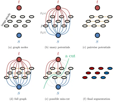
Energy (1.1) can be globally optimized in polynomial time via graph cuts [4]. This can be done by constructing a graph with two special nodes, i.e. source s and sink t, and encoding the unary and pairwise potentials of (1.1) as edge weights. In the constructed graph,sandtrepresent the foreground and background labels, respectively. The optimal segmentation can be computed as a partition of the graph into two disjoint subsets2 _that

minimizes the sum of edge weights between them. This partitioning problem is commonly referred to as the min-cut problem. Now we will briefly cover the graph construction and how to find its min-cut.

Graph Construction:

Unary Potentials (t-links): To construct the graph we begin by adding a node for each image pixel, see Fig. 1.3(a). Each node is then connected to bothsand tvia t-links as illustrated in Fig. 1.3(b). The t-link (s, p) encodes the penalty for assigning p to the

(16)

background, while t-link (p, t) encodes the penalty for assigning p to the foreground. The min-cut will sever one of the two t-links attached to p which defines whether p is connected to the s ort nodes, i.e. pis a foreground or background pixel. For example, if the t-link from thesis severed, the node will only be connected tot and its final labeling will be background.

Pairwise Potentials (n-links): To encode the discontinuity penalties, for each pair of neighbouring pixels/nodes p and q in N we will add an undirected edge, Fig. 1.3(c). Those undirected edges are commonly referred to asn-links. The weight associated with each n-linkis λ.

(a) graph nodes (b) unary potentials (c) pairwise potentials

(d) full graph (e) possible min-cut (f) final segmentation

(17)

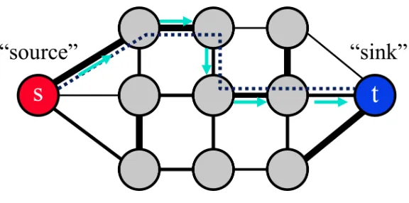
1.2. Binary Segmentation 7

Figure 1.4: Example of a graph with a path from the source s to the sink t.

Min-Cut:

Finding the total weight of the edges in a minimum cut is equivalent to finding the maximum flow in a flow network [10]. Therefore, any maximum flow algorithm can be used to help us solve our binary graph cut problem. In this Section we will explore various maximum flow algorithms.

One of the first maximum flow algorithms developed is Ford-Fulkerson [11]. It is a greedy algorithm that finds and saturates paths (i.e. no more flow can be pushed through the path) fromstot, see Fig. 1.4. The algorithm terminates once all paths are saturated. A downside ofFord-Fulkerson is its time complexity ofO(mf∗), where m is the number of edges in the graph, and f∗ is the maximum flow when capacities are integers. Notice that the time complexity depends on the maximum flow value which could be arbitrarily large depending on the edge weights. Thus, a max-flow algorithm that depends only on the structure of the graph is more preferable thanFord-Fulkerson.

There have been a number of successful attempts to develop algorithms with better time bounds such as Push-Relabel [13], with a time complexity of O(n2m) where n is the number of vertices and m is the number of edges. While there are standard choices for general problems with good theoretical bounds, in practice, it has been found that different algorithms perform better for specific applications. In Computer Vision, the

Boykov-Kolmogorov (BK) algorithm [3] has been shown to outperform general-purpose methods. Despite the lack of a polynomial time bound, BK has been extensively used by the vision community. Recently, an extension of BK was developed that has polynomial time, namedIncremental Breadth First Search (IBFS), which has been shown to be faster than BK in general [12].

(18)

cuts. As a matter of fact, only a subset of pairwise energies can be represented as a graph for which we can compute the max-flow [21, 4]. This subset of energies is commonly referred to as submodular energies. We cover this subset in more detail in Section 1.2.3.

1.2.3 Submodularity

A pairwise energy function is considered submodular if it satisfies the submodularity condition

V(0,0) +V(1,1)≤V(1,0) +V(0,1) ∀(p, q)∈ N. (1.4) The submodularity condition is of significance because submodular pairwise energies can be globally optimized in polynomial time via graph cuts [21]. Moreover, it has been shown in [21] that optimizing non-submodular energies is an intractable problem for general graphs (e.g. on trees it is solvable via dynamic programming).

To prove that energy (1.1) is submodular, we need to show that condition (1.4) is satisfied. By substituting (1.3) into (1.4) we acquire the following inequality

0 + 0 ≤1 + 1

which holds for all (p, q) in N. It is well known that energy (1.1) is submodular for the Ising model (1.3).

1.3 Multi-Label Segmentation

As previously discussed, binary segmentation is limited by its ability to only segment a single object in an image. On the other hand, multi-label segmentation explores the concept of segmenting an image into more than two segments. More precisely, the label set for multi-label segmentation is L={l1, l2, . . . , ln}, wheren > 2.

1.3.1 Energy

Like binary segmentation, multi-label segmentation also involves minimizing an energy with a data term and a smoothness term. Unlike binary segmentation minimizing the energy for multi-label segmentation, even with Potts model (1.3), is NP-hard [4]. The energy for multi-label segmentation is

E(f) =

Data Term

z }| { X

p∈Ω

Dp(fp) +

Smoothness Term

z }| {

λ X

p,q∈N

(19)

1.3. Multi-Label Segmentation 9

where f ={fp ∈ L | ∀p∈Ω}.

The data term is similar to the one defined for binary segmentation (1.2). In terms of pairwise potentials, the greater number of labels corresponds to the possibility of comparing labels in an unordered or ordered fashion. That is, comparing ordered labels may have different costs depending on where the labels lie in the order. Potts model (1.3) is an example of an unordered label comparison. In Potts model the cost of assigning a pair of neighbouring pixels to any two different labels is the same. Potts model could be seen as the generalization of the Ising model to multi-labeling. In the case of ordered labels, e.g. for 1D labels L ⊂ _R1_{, there are pairwise potentials} _V₍_{x, y}_{) =} _g₍_x₋_y_{) such}

that energy (1.1) can be optimized for convex [19] functions g : _R1 _→ _R1_. _For

non-convex g, e.g. Potts model g(t) = [t 6= 0] [4] (where [ ] are the Iverson brackets) or truncated quadratic g(t) =min(t2_{, T}_{) [26] (where} _T _{is some threshold), optimization of}

(1.1) becomes NP-hard on the multi-label cost.

As the multi-label segmentation problem is NP-hard, there are a number of algorithms that attempt to find an approximate solution. One such example isα-expansion [4] which is covered in Section 1.3.2 below.

1.3.2 Optimization via

α-Expansion

One of the most commonly used algorithms to find an approximate solution to multi-label energies in computer vision is α-expansion [4], Alg. 1.

Algorithm 1: α-expansion 1 ˆf ← arbitrary labeling 2 repeat

3 forany (randomly) chosenα∈ L

4 fα ←arg min_f E(f) wheref is anα-expansion of ˆf 5 if E(fα)< E(ˆf)

6 ˆf ←fα

7 until no expansion move reducesE

The α-expansion algorithm begins with an arbitrary labeling ˆf. At each iteration, a label α is chosen at random. On line 4, label α is given the opportunity to expand its support region, i.e. every pixel is given the binary choice to either keep its current labeling or switch toα. The expansion move on line 4 can be formulated asfp =α·xp+ ˆfp·(1−xp)

using the binary labeling x = {xp ∈ {0,1} | p ∈ Ω} that can be solved optimally for

(20)

be improved upon, the algorithm has converged.

There are a number of applications for multi-label segmentation. One such application is image restoration. The problem of image restoration consists of taking a noisy image as input and estimating the original noise-free image. Noise in an image is possible due to many factors, e.g. low light. By using all image intensities as labels, it is possible to “restore” the image using α-expansion as illustrated in Fig. 1.5.

(a) original image (b) noisy image (c) “restored” image

Figure 1.5: Image restoration using α-expansion [4]. The noisy image (b) is taken in as the input, and α-expansion returns an estimated image (c) as the output.

Similar to binary segmentation, not every multi-label pairwise energy can be opti-mized via graph cuts. In Section 1.3.3, we present the conditions under which a multi-label energy can be optimized via α-expansion. In Section 1.4, we present some shape priors used in addition to the smoothness prior to improve segmentation accuracy.

1.3.3 Optimizable Energies via

α-Expansion

In Section 1.2.3, the concept of submodularity was covered as an indicator as to whether a binary pairwise energy function could be optimized in polynomial time or not. With multi-label energy, we are exposed to more general smoothness functions (e.g. convex, truncated convex, etc.). As shown in [4], for such functions to be optimized via α -expansion, the pairwise function must be metric. A function V(fp, fq) is metric on the

set of labels L if it satisfies three constraints:

V(α, β) = 0⇔α=β ∀α, β ∈ L (1.6)

V(α, β) =V(β, α)≥0 ∀α, β ∈ L (1.7)

(21)

1.4. Second-Order Shape Priors 11

These constraints guarantee that the binary expansion moves are submodular and aids in determining if utilizing a particular algorithm is feasible or not. For example, the α-expansion algorithm is only viable for pairwise functions that are metric. Other algorithms, such as the α-β-swap algorithm [4], are more general and could be used for semi-metric energy functions. A semi-metric function is a function that only satisfies (1.6) and (1.7).

There are various shape priors that can be represented as metric pairwise potentials. Examples include star [25] and hedgehog [18] shape priors that will be examined in Section 1.4 below.

1.4 Second-Order Shape Priors

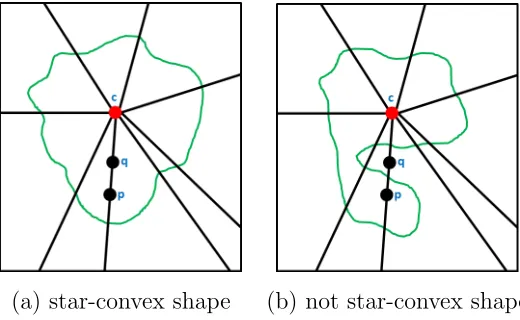
We have covered energy functions that use the image data and smoothness prior. How-ever, users may have further knowledge about the shape of the object to be segmented. It is possible to incorporate that information into the energy function for more accurate results. A common shape prior is the star-shape prior [25] which allows the user to pro-vide information about the shape of the object of interest via a single click identifying its center c. The shape prior guarantees that the segmentation will result in a star-convex shape w.r.t. the centerc. A star-convex shape w.r.t.cmeans that for any pixelp

in the shape, all the pixels along the line betweencand pmust also belong to the shape, see illustration in Fig. 1.6.

(a) star-convex shape (b) not star-convex shape

(22)

Not all objects can be represented using the star-shape prior. Alternatively, the hedgehog shape prior [18] is capable of representing a larger set of shapes. We will give a brief overview of the hedgehog shape prior in Section 1.4.1, since our work extends it.

1.4.1 Hedgehog Shape Prior

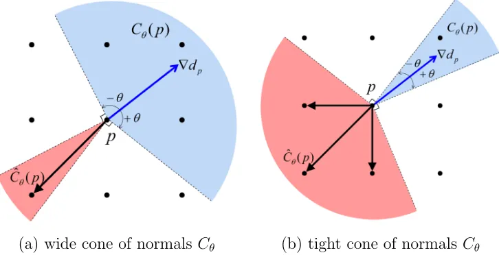
The hedgehog shape prior locally constrains normals of points on the surface of the segment using a reference vector field. As explored in [18] there is more than one way to generate the reference vector field. For example in [18], the reference vector field was the gradient of the distance map of the user-scribble/seed. Unlike the star-shape prior, a hedgehog seed is not restricted to being a single point. In contrast to the star-shape prior, the hedgehog prior utilizes a shape tightness parameterθthat gives the user control over the set of feasible shapes.

(a) user-seed & its distance map d (b) Hedgehog constraint _∠(¯nS

p,∇dp)≤θ

Figure 1.7: Hedgehog constraints [18] for segment S. (a) user-seed defines a signed distance mapd. (b) surface normals ¯nS

p of S are constrained by ∠(¯npS,∇dp)≤θ.

Figure 1.7 illustrates the hedgehog constraint:

∠(¯nS_p,∇dp)≤θ ∀p∈∂S, (1.9)

where ¯nS

p is the normal of the surface of segmentS atp, ∇dp is the reference vector field

atpand∂S is the boundary ofS. Now we will give a brief overview on how the hedgehog constraints (1.9) were formulated as pairwise potentials in [18].

Let us consider the area in which the surface normal may fall as the cone of allowed surface normals Cθ(p),

(23)

1.4. Second-Order Shape Priors 13

(a) wide cone of normals Cθ (b) tight cone of normals Cθ

Figure 1.8: shows how to approximate hedgehog constraint at pixelp. ConeCθ(p) of the

allowed surface normals (blue) is enforced by ensuring that all the neighbouring pixels in the corresponding polar coneCb_θ(p) (red) lie insideS if p∈S.

at some pixel p, see the illustration in Fig. 1.8 for two different values of θ. It is easy to see that the boundary of segment S atp has normal ¯nS

p ∈Cθ(p) iffthe surface of S does

not pass through the corresponding polar cone Cbθ(p),

b

Cθ(p) := {y| h(p, y),(p, z)i ≤0 ∀z ∈Cθ(p)}. (1.11)

With this in mind, it is easy to approximate the hedgehog constraint (1.9) as pairwise potentials. Simply, the hedgehog constraint atpboils down to the following: ifpbelongs to segment S then all neighbouring points of p that lie in Cb_θ(p) must also lie inside S. LetE(θ) be the set of hedgehog constraints edges,

E(θ) = {(p, q)|(p, q)∈ Cbθ(p) ∀(p, q)∈ N }. (1.12)

The shape tightness parameter θ is used to control how close the final segmentation is to the level sets of the distance map of the seed. Whenθ is 0, the set of feasible shapes will be the levels sets of the distance map d. As θ increases, the set of feasible shapes increases, see [18] for more details.

The hedgehog shape prior can be added to (1.5) as follows:

E(f) =

Data Term

z }| { X

p∈P

Dp(fp) +

Smoothness Term

z }| {

λ X

p,q∈N

V(fp, fq) +

Shape Prior Term

z }| {

Hθ(f) (1.13)

where

Hθ(f) =

X

k∈L

X

(p,q)∈Ek(θ)

(24)

and [ ] are the Iverson brackets, w∞ is a prohibitively expensive weight, and Ek

corre-sponds to the hedgehog shape prior for the boundary of label (object)k. If the proposition inside the Iverson bracket is true it returns 1 and 0 otherwise.

1.5 Prior Work Limitations

In previous sections, we explored the concepts of binary and multi-label segmentation. We now look at the drawbacks of the corresponding optimization algorithms in light of the hedgehog prior. For simplicity, we will focus on binary segmentation but the findings extend to multi-label segmentation as well.

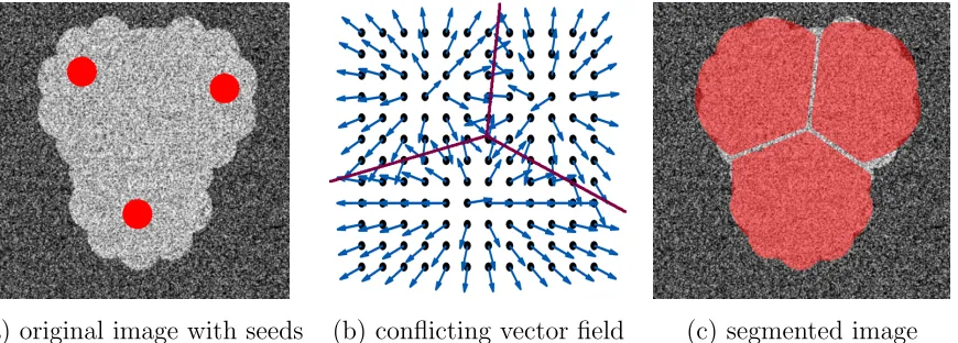
In the context of binary segmentation with hedgehogs, a problem arises when the user seeds/scribbles are complex, e.g. a seed with multiple disconnected parts, see Fig. 1.9(a). As reported in [16], such complex seeds usually results in a non-smooth vector field which leads to segmentation errors, see Fig. 1.9(c), due to conflicting hedgehog constraints along the vector field discontinuities, see Fig. 1.9(b).

(a) original image with seeds (b) conflicting vector field (c) segmented image

Figure 1.9: (a) synthetic example with a complex seed (red). (b) non-smooth vector field that leads to conflicting hedgehog constraints (highlighted by the red lines). Note that due to over-constraints, no segmentation can pass through the red lines on (b) leading to (c) incorrect segmentation of [18].

To overcome the issue of conflicting constraints, we propose using multiple smooth

(25)

1.6. Thesis Contributions 15

1.6 Thesis Contributions

The main contributions of this thesis are:

• A new segmentation model that allows overlapping labels, namely Segmentation with Overlapping Labels (SOL). This model is well-suited for segmenting multi-part foreground objects where each multi-part has an independent shape prior. We show that solving image segmentation while allowing labels to overlap is an NP-hard problem.

• To approximately optimize SOL, we propose an optimization framework that uses our novel combinatorial moves,Expansion-Contractionmoves (EC-moves).

• We evaluate our approach on synthetic examples and real data, i.e. liver segmenta-tion in CT-scans. We also compare our results to state of the art algorithms using Potts model (α-expansion with and without the Hedgehog shape prior).

1.7 Thesis Outline

(26)

SOL: Segmentation with

Overlapping Labels

(27)

2.1. Overview and Motivation 17

2.1 Overview and Motivation

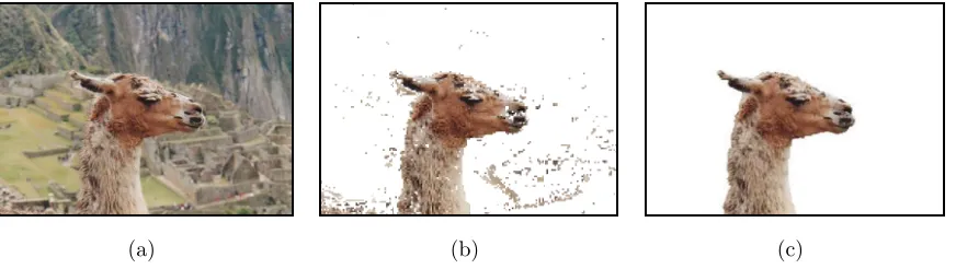
In Section 1.5, we exposed some issues with the classical segmentation model where segments are mutually exclusive. To summarize, using complex seeds (e.g. disjoint seeds) for a hedgehog shape prior [18] often results in a segmentation that does not accurately cover the object [18, 16] as illustrated in Fig. 2.1. More precisely, for complex seeds, e.g. multi-part seed shown in Fig. 2.1(a), the resulting distance map is not continuous as shown in Fig. 2.1(b). Thus, the gradient of the distance map is a non-smooth vector field, see Fig. 2.1(c). Using a non-smooth vector field to impose the hedgehog constraints (1.9) results in conflicting constraints along the distance map discontinuities, which in turn results in an incorrect segmentation, see Fig. 2.1(d).

(a) complex seed (b) distance transform

(c) non-smooth vector field (d) segmentation result [18]

(28)

In an attempt to avoid discontinuities in the distance map, we explored the idea of splitting complex seeds into multiple simple ones with different labels resulting in contin-uous distance maps. Instead of segmenting one foreground label using complex seeds, we propose separately segmenting n foreground parts/labels, each with a simple seed. For instance, the complex seed shown in Fig.2.1(a) could be split into three parts/labels, as shown in Fig. 2.2, top row. As you can see the resulting independent vector fields are smooth and do not lead to conflicting hedgehog constraints.

(29)

2.1. Overview and Motivation 19

On the one hand, splitting complex seeds into multiple simple ones eliminates the issue of conflicting hedgehog constraints. On the other hand, the globally optimizable binary segmentation problem transforms into an NP-hard multi-labeling problem, see Section 1.3. It is possible to use α-expansion to obtain an approximate solution. How-ever, in practice we found that α-expansion usually converges to poor local minima, see Figure 2.3(b). We mainly attribute this poor performance to using the classical segmen-tation model that assumes independent mutually exclusive labels. In the context of our application, the independence assumption does not hold. This is due to the fact that our foreground labels/parts represent the same foreground object but each label has its own hedgehog constraints.

(a) seeds (b) local minima of α-expansion (depending on the initialization)

(c) seeds (b) different local minima of our proposed method

Figure 2.3: (b) shows the three different local minima found by α-expansion with the Hedgehog constraint when enforcing mutually exclusive foreground labels. Note the over-segmentation of the first expansion and under-over-segmentation of subsequent expansions. (d) shows the three different local minima of our proposed method (allowing foreground labels to overlap) with the Hedgehog constraint.

(30)

2.2 SOL Energy

We will start by redefining some notation. Let Ω be the set of all image pixels, and

L = {B, F1, . . . , Fn} be set of all labels where B and Fi are the background and the ith

foreground part, respectively. Let γB and γF denote the Gaussian mixture color model

of the background and foreground labels, respectively. In the context of our application, all foreground parts have the same color model but they could be different if needed.

Figure 2.4: depicts a possible segmentation with three foreground labels (F1, F2, F3) and

one background label B, represented by fk

p for each pixel p. Furthermore, the hatched

(31)

2.2. SOL Energy 21

Let f = {fk

p| ∀p ∈ Ω, k ∈ L} be a labeling of Ω where fpk is a binary variable that

indicates whether pixel p is assigned to label k or not, i.e.

f_pk =  



1 pixelp is assigned to k∈ L

0 otherwise.

By defintion, f allows a pixel to be assigned to more than one label. However, in the context of our application we only allow a pixel to be assigned to either the background or at least one of the foreground labels, i.e.

f_pB =

n

Y

i=1

(1−fFi

p ) ∀p∈Ω.

We will further introduce an indicator variable fp ∈ {B,F } to indicate whether p is

assigned to the background label or not, refer to Figure 2.4. More specifically, if a pixel is assigned to any number of foreground labels, fp = F, and if a pixel is assigned to

the background label, fp = B. Technically fp is equivalent to fpB as fpB = 0 means that

fp =B. However, we use the symbolsB and F instead of 0 and 1 for notational clarity.

Our multi-part foreground segmentation energy of SOL is

E(f,

γ

B,

γ

F) =

data term

z }| { X

p∈Ω

Dγ_p(fp) +

smoothness term

z }| {

λ X

p,q∈N

wpq[fp 6=fq] +

hedgehog constraints

z }| {

Hθ(f), (2.1)

where λ is a normalization constant, N is the pixels’ neighbour system, wpq is the

dis-continuity cost, [ ] are the Iverson brackets, and Hθ(f) represents the hedgehog shape

constraints. For SOL we define the hedgehog constraints as:

Hθ(f) =

X

k∈L\B X

(p,q)∈Ek(θ)

w∞[fpk = 1, f k

q 6= 1], (2.2)

where w∞ is a very large constant, Ek(θ) is the set of edges used to approximate the

hedgehog shape prior constraint (1.12) for label k, andθ is the tightness of the hedgehog constraints (1.9). The three terms of our energy are discussed in further details below.

The first term in our energy is usually referred to as the data term or the regional term. Dγp(fp) is the cost of assigning pixelp to label fp and usually computed as:

Dγ_p(fp) =− ln Pr(Ip |

γ

fp), (2.3)

whereP r is the probability of the color intensity Ip at pixelpgiven the color model γfp.

(32)

only pay the cost of being assigned to the foreground once. It will use a color model derived from all the foreground seeds. Conceptually, a pixel with multiple foreground labels simply reduces to a pixel labeled foreground.

The smoothness term in (2.1) is used to discourage label discontinuities between neighbouring pixels. Our smoothness term is somewhat different from the commonly used Potts model [4] for multi-label segmentation. In Potts model, a pair of neighbouring pixels pays for a discontinuity if they are assigned to two different labels. In contrast, in our smoothness model, a pair of neighbouring pixels pays for a discontinuity only between background and non-background labels. The discontinuity cost wpq between p

and q is a non-negative weight that is application specific.

The final term in our energy imposes hedgehog constraints on each foreground label individually. Each foreground label has its surface normals locally constrained by a vector field1_{. This is in contrast to [18] where the foreground was restricted by a single vector}

field which occasionally resulted in segmentation errors, see Fig. 2.1.

2.3 SOL Optimization

We propose Grabcut for Overlapping-Labels (GOL), Alg. 2, to find an approximate solution to (2.1). Initially, the user provides seeds denoting each individual foreground label and the background. Similar to [24], we start from a trivial solution2 _{and optimize}

(2.1) in block-coordinate descent. Specifically, our framework alternates between (a) fixing current labeling ˆf and optimizing color models γB and γF, and (b) fixing the color models and optimizing labeling f. Our framework stops when both steps no longer decrease (2.1).

As shown in GOL step 4, given current labeling ˆf, we use the EM-Algorithm [9] to re-estimate the foreground and background color models. In step 5, given γB and γF, optimizing (2.1) reduces to a multi-labeling problem that allows labels to overlap which is NP-hard, see proof in Section 2.5. One of the main contributions of this work and a key step in GOL is Alg. 3 Expansion-Contraction Moves (EC-Moves). Given γB and

γF, EC-Moves finds an approximate labeling to energy (2.1) via a series of binary moves.

1_{In our case, it is the gradient of the user-scribble’s distance map.}

(33)

2.4. Binary Optimization Moves 23

Algorithm 2: Grabcut for Overlapping-Labels (GOL)

1 Input: ˆf ← trivial initial labeling (user-seeds) 2 E∗ ← ∞

3 repeat

4 γB, γF ← Re-estimate color models given ˆf using EM

5 ft ←arg min_f E(f, γB, γF) given γB and γF using EC-Moves(Alg. 3) 6 if E(ft, γB, γF)< E∗

7 ˆf ←ft

8 E∗ ←E(ft, γB, γF)

9 until converged (no decrease in E) 10 return ˆf

Algorithm 3: Expansion-Contraction Moves (EC-Moves)

1 Input: ˆf ← current labeling 2 repeat

3 α ← random label ∈ L \ B ≡ {F1,· · · , Fn}

4 if coin toss is heads

5 fα ← arg minf E(f) wheref is an α-expansion of ˆf 6 else

7 fα ← arg min_f E(f) wheref is an α-contraction of ˆf 8 if fα <ˆf

9 ˆf ←fα

10 until converged (no decrease for allα ∈ L)

The EC-Moves Alg. randomly traverses the foreground labels. At every iteration, an arbitrarily labelαrandomly chooses to either expand or contract its support region. The current labeling is updated if the expansion (or contraction) results in a lower energy. EC-Moves terminates when no move leads to a new labeling with a lower energy. The expansion and contraction moves used in EC-Moves are elaborated on in Section 2.4.

2.4 Binary Optimization Moves

(34)

contraction which may only switch to the single background label (or stay the same). Although background expansion is a binary move, utilizing it did not affect the results in practice.

2.4.1 α-Expansion Move:

(a) current segmentation (b) a feasible α-expansion move on F1

Figure 2.5: (a) shows a sample of a current segmentation. (b) shows a feasible expansion for label F1. Notice howF1 expands while F2 and F3 remain unaffected.

In an expansion move on a foreground labelα ∈ L \ B ≡ {F1,· · · , Fn}, a pixel is given a

binary choice that depends on whether it is currently a background or foreground pixel. A currently labeled background pixel is given the choice to either stay the same or switch toα. A currently labeled foreground pixel is given the choice to either stay the same or add α to its set of foreground labels.

Figure 2.5 illustrates an example of a possible expansion on the label F1. There

are three things to note about pixels that were affected by the expansion. First, some background pixels decided to switch to F1. Secondly, some foreground pixels that did

not include F1 added F1 to their list of foreground labels. Lastly, no other foreground

label, i.e. F2 and F3, gained or lost any pixels.

Given the current labeling ˆf and color models γF and γB, an expansion move on

α∈ {F1,· · · , Fn} can be formulated as a binary energy as follows:

E_αe(x) = X

p∈Ω

Dγ_p ( ˆfp)xp+Dγp (α)xp+λ

X

p,q∈N

wpqV(xp, xq) +

X

(p,q)∈Eα(θ)

(35)

where x={xp ∈ {0,1} | ∀p∈Ω}, ifxp is 1 then a pixel switches to α,

V(xp, xq) =

          

[ ˆfp 6= ˆfq] if xp = 0, xq = 0

[B= ˆfq] if xp = 1, xq = 0

[ ˆfp =B] if xp = 0, xq = 1

0 if xp = 1, xq = 1

(2.5)

and

S(u, v) = (

w∞ if u= 1, v = 0

0 otherwise. (2.6)

Submodularity

To prove that (2.4) is submodular we need to prove that V(xp, xq) and S(u, v) are

sub-modular for any α∈ L \ B ≡ {F1,· · · , Fn}. We will first considerV(xp, xq) as defined in

(2.5). For V to be submodular it must satisfy the submodularity condition (1.4), i.e.

V(0,0) +V(1,1)≤V(0,1) +V(1,0) (2.7) [ ˆfp 6= ˆfq] + 0≤[ ˆfp =B] + [ ˆfq =B] by substituting (2.5). (2.8)

Inequality (2.8) depends on the current labeling of pixels p and q, i.e. ˆfp and ˆfq. As

such, to show that (2.8) always holds we will consider all possible variations of ˆfp and

ˆ

fq. As a pixel’s labeling can be either F or B, we have the following cases to consider

if fˆp =B,fˆq =B then 0 + 0≤1 + 1

if fˆp =F,fˆq =B then 1 + 0≤0 + 1

if fˆp =B,fˆq =F then 1 + 0≤1 + 0

if fˆp =F,fˆq =F then 0 + 0≤0 + 0.

For all possible cases, we can see that the submodularity constraint holds so we can claim that V(xp, xq) is submodular.

To prove that S(u, v) is submodular the submodularity constraint (2.8) must hold

S(0,0) +S(1,1)≤S(0,1) +S(1,0) (2.9) 0 + 0≤0 + 1 by substituting (2.6). (2.10) Therefore,S(u, v) is submodular. Since bothV(xp, xq) andS(u, v) are submodular then

(36)

2.4.2 α-Contraction Move:

(a) current segmentation (b) a feasible α-contraction move on F1

Figure 2.6: (a) shows a sample of a current segmentation. (b) shows a feasible contrac-tion for labelF1. Notice howF1 loses pixel support whileF2 and F3 remain unaffected.

In a contraction move on any foreground label α∈ L \ B ≡ {F1,· · · , Fn}, every pixel

has a binary choice depending on its current labelling. On the one hand, a pixel only labeled α is given the choice to either stay the same or switch to the background label. On the other hand, any other pixel is given the choice to either stay the same or remove

α from its set of labels, if it was there.

Figure 2.6 illustrates an example of a possible contraction on the label F1. There

are three things to note about pixels that were affected by the contraction. First, some pixels that were only labeled F1 decided to switch to the background label. Secondly,

some pixels that were assigned to multiple foreground labels including α lost their α

label but maintained their other foreground labels. Lastly, no other foreground label gained or lost any pixels (i.e. their labeling stayed the same). It is worth mentioning that pixels with multiple foreground labels that did not include α would not be affected by the contraction.

To simplify our notation, we use an indicator variable δp that depends on the current

labeling to indicate whether a pixel p isonly labeled α or not:

δp =

(

1 ∀k ∈ L \α, fˆk p = 0

0 ∃k ∈ L \α s.t. ˆfk p = 1.

(37)

Given current labeling ˆf, a contraction move on α can be formulated as:

E_αc(x) =

pixels assignedonlytoα

z }| {

X

p∈Ω

δp=1

Dγ_p( ˆfp)¯xp +Dγp(B)xp+

other pixels

z }| { X

p∈Ω

δp=0

Dγ_p( ˆfp) +

λ X

p,q∈N

wpqV(xp, xq) +

X

(p,q)∈Eα(θ)

S(xq, xp) (2.12)

whereS(u, v) is as previously defined in (2.6) andV(xp, xq) is a binary pairwise potential

defined as

V(xp, xq) =

          

[ ˆfp 6= ˆfq] if xp = 0, xq= 0

[ ˆfp 6=B]δq+ [ ˆfp = ˆ6 fq] ¯δq if xp = 0, xq= 1

[B 6= ˆfq]δp+ [ ˆfp = ˆ6 fq] ¯δp if xp = 1, xq= 0

[ ˆfp 6= ˆfq] ¯δpδ¯q+ [B 6= ˆfq]δpδ¯q+ [ ˆfp 6=B] ¯δpδq if xp = 1, xq= 1.

(2.13)

Figure 2.7: (a) the hatched area shows the pixels that may change their data term in a contraction (i.e. switch from foreground to background). Pixel p is a part of this set and pixel q is not. (b) shows an example of a feasible contraction. Notice that for pixel

p, the data term changed to background while pixel q remained foreground.

Figure 2.7 illustrates the different choices given to pixels p and q during an α = F1

contraction. Pixelpfalls under the set of pixels that are only labeledF1, i.e. the hatched

area in Fig. 2.7(a). Pixels in this area have the option to switch fromF1to the background

or to stay the same. Pixel q is not only labeled F1 and thus, it is given the option to

(38)

which both pixel p and pixel q decided to lose their the F1 label. Pixel p switched to

background while q remained foreground but F1 is no longer part of its foreground label

set.

Submodularity

To prove that (2.12) is submodular we need to prove that V(xp, xq) and S(u, v) are

submodular. In order for V(xp, xq) to be submodular it must satisfy the submodularity

condition (1.4), i.e.

V(0,0) +V(1,1)≤V(0,1) +V(1,0). (2.14) By substituting (2.13) in (2.14)

[ ˆfp 6= ˆfq] + [ ˆfp 6= ˆfq]¯δpδ¯q+ [B 6= ˆfq]δpδ¯q+ [ ˆfp 6=B]¯δpδq≤

[B 6= ˆfq]δp+ [ ˆfp 6= ˆfq]¯δp + [ ˆfp 6=B]δq+ [ ˆfp 6= ˆfq]¯δq. (2.15)

Inequality (2.15) depends on the current labeling of p and q, i.e. ˆfp and ˆfq.

Further-more, (2.15) also depends on the indicator variablesδp and δq. Thus, to show that (2.15)

always hold will consider all possibilities of ˆfp, ˆfq, δp and δq. There are only 9 cases to

check as the other remaining cases will lead to invalid configuration, e.g. ˆfp = B while

δp = 1. The 9 valid cases are

if fˆp =B, fˆq =B, δp = 0, δq= 0 then 0 + 0 + 0 + 0≤0 + 0 + 0 + 0

if fˆp =F, fˆq =B, δp = 1, δq = 0 then 1 + 0 + 0 + 0≤0 + 0 + 0 + 1

if fˆp =F, fˆq =B, δp = 0, δq = 0 then 1 + 1 + 0 + 0≤0 + 1 + 0 + 1

if fˆp =B, fˆq =F, δp = 0, δq = 1 then 1 + 0 + 0 + 0≤0 + 1 + 0 + 0

if fˆp =B, fˆq =F, δp = 0, δq = 0 then 1 + 1 + 0 + 0≤0 + 1 + 0 + 1

if fˆp =F, fˆq =F, δp = 1, δq = 1 then 0 + 0 + 0 + 0≤1 + 0 + 1 + 0

if fˆp =F, fˆq =F, δp = 0, δq = 0 then 0 + 0 + 0 + 0≤0 + 0 + 0 + 0.

(39)

2.5. NP-Hardness Proof 29

2.5 NP-Hardness Proof

In general, the SOL problem is NP-hard. To prove this we will reduce the Set Cover problem instance to SOL in polynomial time, i.e. Set Cover ≤P SOL. In a Set Cover

problem we are given a set of n elements that forms universe U = {u1, u2, . . . un}, and

a set of m subsets S = {Si ⊆ U | ∀i ∈ [1, m]}. The aim is to find the least number of

subsets such that their union covers the universe U.

A SOL problem (2.1) is defined by the pixel set Ω, the label set L, the data term

Dγp(fp), the neighbourhood system N, and the set of hedgehog constraints E. Given

U and S of a Set Cover problem we can construct the corresponding SOL problem as follows:

Pixel set: Ω := {U ∪ A} where A = {ai | ∀i ∈ [1, m]}. A is a set of auxiliary

pixels/nodes. In this section will refer to pixels as nodes. For each set Si, we introduce

an auxiliary nodeai that will be used as an indicator of whetherSi is one of the selected

sets to cover U or not.

Label set: L := {B ∪ {Fi | ∀i ∈ [1, m]}} where the label Fi corresponds to subset Si

and B is the background label. In the context of the Set Cover problem the background label serves no purpose but it was kept for ease of juxtaposition to the SOL problem.

Data term: We define the data term as follows

Dγ_u(`) =                 

∞ ∀u∈Ω, `=B (2.16) 0 ∀u∈Si, `=Fi ∀i∈[1, m] (2.17)

∞ ∀u6∈Si, `=Fi ∀i∈[1, m] (2.18)

1 u=ai, `=Fi ∀i∈[1, m] (2.19)

0 u=ai, `=Fj ∀i, j ∈[1, m], i6=j. (2.20)

In (2.16) the data term prohibits any node to be assigned to the background label B. In (2.17) and (2.18) the data term prohibits a nodeu6∈Si to be given the labelFi.In (2.19)

and (2.20) the data term ensures that our energy increases by 1 if ai is give the label Fi.

(40)

Hedgehog constraints: For a given set Si we define the corresponding hedgehog

con-straints EFi of labelFi as follows:

EFi :=CFi∪ IFi

, where the set of connectedness constraints is CFi :={(u, v)| ∀u, v ∈ Si, u6=v} and the

set of indicatorconstraints is IFi :={(u, ai)| ∀u∈Si, ai ∈A}. The edges

3 _in _C

Fi ensure

that if a node u ∈ Si is given the label Fi then every other node in the set Si will also

be given label Fi. The edges in IFi ensures that if any node u∈Si is given the label Fi

then the corresponding auxiliary node ai of Si is given the label Fi as well.

Objective: The objective in Set Cover is to minimize the number of selected subsets to cover U, which is the energy of the corresponding SOL problem. Notice that if a node

u ∈ Si decides to be given the label Fi then ai will be will also be given the label Fi.

And, since Daγi(Fi) = 1 by definition then we can conclude that our energy counts the

number of subsets appearing in the final solution. Recall that there is no smoothness term and that the hedgehog term is 0 or ∞.

(41)

Chapter 3 Experiments

(42)

Our experiments were conducted on both synthetic examples as well as real data (CT scans of the liver). We used these examples to compare α-expansion [4] and its various modifications (i.e. adding a shape prior [18], allowing overlapping labels) with our approach. The same parameters were used for all approaches to ensure an accurate comparison. Further, this guaranteed that our final energy would be comparable.

3.1 Synthetic Example

We compare our approach for segmenting the synthetic example shown in Fig. 3.1 to [4, 18]. For all methods we utilized the same parameters, namely, θ = 20, N was the 4-neighbourhood system, and λ = 2. The initial foreground and background color models were calculated using user-seeds. The pairwise discontinuity penalty between neighbouring pixels pand q, i.e. wpq, was set to 1.

(a) original image (b) ground truth

Figure 3.1: (a) depicts our original synthetic image while (b) displays the ground-truth segmentation.

(43)

3.1. Synthetic Example 33 Classical Segmen tation                                                    Binary[18]

E = 12,147,526,642

α

-Exp[4]

E = 12,987,975,367 E = 12,868,749,100 E = 13,080,701,611

                                                   SOL α -Exp

E = 12,314,319,653 E = 12,204,283,336 E = 12,225,621,607

EC

Mo

v

es

E = 11,983,387,407 E = 11,983,597,499 E = 11,983,451,254

(44)

The second row in Figure 3.2 corresponds to the classical α-expansion [4]. The first column depicts the initial seeds. In contrast to the binary segmentation, the seeds are assigned to separate labels. The following columns show three different local minimas depending on the order of the expanding labels. It can be seen that this algorithm suffers from local minima in which the first expanding label attempts to cover the entire object, preventing the other labels from expanding.

The third row in Figure 3.2 corresponds to a modification of α-expansion in which foreground labels are given the freedom to overlap. As the idea of overlapping labels has not been previously explored, we used our own implementation for this experiment and cover the results for the sake of comparison. It can be seen that allowing labels to overlap alleviates the local minima issue by allowing subsequent labels to expand further but the segmentation is still sensitive w.r.t. the order of expanding labels. This is due to a limitation in the background expansion, i.e. it does not allow pixels with multiple foreground labels to lose one of those foreground labels. The contraction moves we propose overcomes this problem by replacing the background expansion by a series of foreground labels contractions.

The final row in Figure 3.2 corresponds to our approach that uses the novel contraction moves. It can be seen that this provides a segmentation that is more robust towards the order of the expansion sequence. It is visually clear that our approach results in a better segmentation overall as labels are not expanding further than the edge of the object. As all experiments were run with the same parameters, the final energy is comparable across the different segmentation models/optimization frameworks and it can be seen that our approach finds the solution with lowest energy amongst them.

3.2 Liver Segmentation

Given a 2D CT slice, we compare the segmentation of the liver from the rest of the organs. We examined 6 separate subjects, comparing three different approaches:

• Approach 1 (A1): α-expansion (without overlapping labels) [4]

• Approach 2 (A2): α-expansion (without overlapping labels) with a shape prior [4, 18]

• Approach 3 (A3): our approach

(45)

3.2. Liver Segmentation 35

models. For the shape prior we used hedgehog with θ = 30. Finally, the smoothness term λ was set to 5 and we used canny edges to derive the discontinuity cost wpq.

Canny-edges [6] is an edge detection operator, see Fig. 3.3. Canny-edges provides valuable information as to where the object boundary should occur, which may be incor-porated into the pairwise discontinuity cost. The idea is to have a smaller discontinuity penalty along canny edges in comparison to discontinuities elsewhere. That is, if E is the set of edge pixels detected by Canny-edges then

wpq =

 



0.25 (p∈E, q /∈E)∨(q ∈E, p /∈E) 1 (p∈E, q∈E)∨(p /∈E, q /∈E)

(3.1)

where the 0.25 penalty is heuristically chosen. Decreasing the heuristically chosen weight encourages discontinuities to occur along the Canny-edges.

(a) original image (b) set of Canny-edges pixels show in white

Figure 3.3: (a) is the input image. (b) shows the output of the Canny-edges algorithm [6], the set of edge pixels, E, is shown in white.

(46)

(a)

(b) A1 Energy = 6163304098 (c) A2 Energy = 6374004875

(d) A3 Energy = 5328368114 (e)

(47)

(a)

(d) A3 Energy = 3360526210 (e)

(48)

(a)

(d) A3 Energy = 4122849903 (e)

(49)

(a)

(d) A3 Energy = 6149069898 (e)

(50)

(a)

(d) A3 Energy = 6427667575 (e)

(51)

(a)

(d) A3 Energy = 4654115540 (e)

(52)

For quantitative comparison, we calculate the precision and recall for each segmenta-tion which are reported in Table 3.1. We calculate these values in relasegmenta-tion to a manually segmented ground truth. Precision calculates the ratio between the number of true pos-itives versus the total number of pospos-itives, i.e

Precision = true positive

true positive + false positive.

Recall calculates the ratio between the number of true positives versus the total number of labeled pixels, i.e.

Recall = true positive

true positive + false negative.

Subject Metric classic segmentation SOL A1 [4] A2 [4, 18] A3 (Ours)

Subject 1 Precision 0.690 0.935 0.971 Recall 0.989 0.660 0.973

Table 3.1: Precision and Recall values for the various subjects (subjects 1 - 6) and approaches (A1 - A3).

In Table 3.1, it can be seen that A1 consistently has the highest recall values while maintaining consistently low precision values. This is compatible with what can be seen in the figures where A1 over-segments the image such that much of the liver is properly labeled, but many portions of the scan are incorrectly labeled as liver. It should be noted that it is possible to fine-tune λ to acquire better results for A1 but we used the same λ

(53)

While the segmentation for A2 improves the precision values, the recall values de-crease. It can be seen that this is due to the local minima issues that were explained in Section 3.1, causing the liver to be under-segmented.

Finally, A3 not only has the highest precision values, but also maintains recall values which are comparable to A1. As with A2, A3 benefits from the shape prior, resulting in high precision values. However, as it allows overlaps between the foreground labels, it avoids weak local minima. For ease of comparison, Figure 3.10 displays a graphical representation of the precision vs. recall for each algorithm and shows how A3 consistently outperforms both A1 and A2.

Figure 3.10: Graphical representation of precision vs. recall values for the three ap-proaches (A1 - A3).

Lastly, Table 3.2 displays the F1 score. The F1 Score is a common metric to quantify

the closeness of the segmentation to the ground truth. It combines the precision and recall values into a single value where an exact correspondence to the ground truth is 1. It is calculated as

F1 Score = 2·

(54)

Sub. 1 Sub. 2 Sub. 3 Sub. 4 Sub. 5 Sub. 6

A1 [4] 0.812 0.554 0.609 0.695 0.783 0.770

A2 [4, 18] 0.774 0.749 0.847 0.894 0.772 0.877

A3 (Ours) 0.972 0.935 0.896 0.976 0.942 0.940

(55)

Chapter 4 Future Work and Conclusion

(56)

In this work. we have introduced the concept of segmentation with overlapping labels, a segmentation model that excels at segmenting translucent objects, occluded objects, and objects that require multiple seeds. Specifically, we have shown that SOL is an effec-tive segmentation model for segmenting complex objects with multiple parts. Further, we have proved that SOL is an NP-hard problem and provided an iterative algorithm to find an approximate solution.

Our approach was inspired by theα-expansion [4] and grab-cut algorithms [24]. How-ever, our optimization framework utilizes the novel expansion and contraction moves. To test our algorithm, we ran several experiments on both synthetic images as well as medi-cal images. The results of these experiments display the advantage of using our approach in comparison to the state-of-the-art methods.

(a) source image (b) expected SOL segmentation Figure 4.1: (a) depicts an image of cells that may benefit from SOL over mutually exclusive labels. (b) shows an expected SOL segmentation.

Cell segmentation is a possible application of SOL. The concept of overlapping labels is particularly useful in medical imaging where objects are translucent, see in Fig. 4.1. This property make it difficult, if not impossible, for the classic segmentation model to properly segment each cell as a separate label.

(57)

Bibliography

[1] A. Berman, A. Dadourian, and P. Vlahos. Method for removing from an image the background surrounding a selected object, October 17 2000. US Patent 6,134,346.

[2] Christopher M Bishop. Pattern recognition and machine learning (information sci-ence and statistics) springer-verlag new york. Inc. Secaucus, NJ, USA, 2006.

[3] Yuri Boykov and Vladimir Kolmogorov. An experimental comparison of min-cut/max-flow algorithms for energy minimization in vision. IEEE transactions on pattern analysis and machine intelligence, 26(9):1124–1137, 2004.

[4] Yuri Boykov, Olga Veksler, and Ramin Zabih. Fast approximate energy minimization via graph cuts. IEEE Transactions on Pattern Analysis and Machine Intelligence, 23:1222–1239, November 2001.

[5] Yuri Y Boykov and M-P Jolly. Interactive graph cuts for optimal boundary & region segmentation of objects in nd images. In Computer Vision, 2001. ICCV 2001. Proceedings. Eighth IEEE International Conference on, volume 1, pages 105– 112. IEEE, 2001.

[6] John Canny. A computational approach to edge detection. IEEE Transactions on pattern analysis and machine intelligence, (6):679–698, 1986.

[7] D. Cremers, T. Pock, K. Kolev, and A. Chambolle. Convex relaxation techniques for segmentation, stereo and multiview reconstruction. In Markov Random Fields for Vision and Image Processing. MIT Press, 2011.

[8] Andrew Delong and Yuri Boykov. Globally optimal segmentation of multi-region objects. In Computer Vision, 2009 IEEE 12th International Conference on, pages 285–292. IEEE, 2009.

(58)

[9] Arthur P Dempster, Nan M Laird, and Donald B Rubin. Maximum likelihood from incomplete data via the em algorithm. Journal of the royal statistical society. Series B (methodological), pages 1–38, 1977.

[10] Lester R Ford and Delbert R Fulkerson. Maximal flow through a network. Canadian journal of Mathematics, 8(3):399–404, 1956.

[11] Lester Randolph Ford Jr and Delbert Ray Fulkerson. Flows in networks. Princeton university press, 2015.

[12] Andrew V Goldberg, Sagi Hed, Haim Kaplan, Pushmeet Kohli, Robert E Tarjan, and Renato F Werneck. Faster and more dynamic maximum flow by incremental breadth-first search. In Algorithms-ESA 2015, pages 619–630. Springer, 2015.

[13] Andrew V Goldberg and Robert E Tarjan. A new approach to the maximum-flow problem. Journal of the ACM (JACM), 35(4):921–940, 1988.

[14] Lena Gorelick, Olga Veksler, Yuri Boykov, and Claudia Nieuwenhuis. Convexity Shape Prior for Segmentation, pages 675–690. Springer International Publishing, Cham, 2014.

[15] Lena Gorelick, Olga Veksler, Yuri Boykov, and Claudia Nieuwenhuis. Convexity shape prior for binary segmentation. IEEE transactions on pattern analysis and machine intelligence, 39(2):258–271, 2017.

[16] Hossam Isack, Yuri Boykov, and Olga Veksler. A-expansion for multiple” hedgehog” shapes. Technical report, 2016.

[17] Hossam Isack, Olga Veksler, Ipek Oguz, Milan Sonka, and Yuri Boykov. Efficient optimization for hierarchically-structured interacting segments (HINTS). In IEEE Conference on Computer Vision and Pattern Recognition, 2017.

[18] Hossam Isack, Olga Veksler, Milan Sonka, and Yuri Boykov. Hedgehog shape priors for multi-object segmentation. InIEEE Conference on Computer Vision and Pattern Recognition, 2016.

[19] Hiroshi Ishikawa. Exact optimization for markov random fields with convex priors.

(59)

BIBLIOGRAPHY 49

[20] Jesmin F Khan, Sharif MA Bhuiyan, and Reza R Adhami. Image segmentation and shape analysis for road-sign detection. IEEE Transactions on Intelligent Trans-portation Systems, 12(1):83–96, 2011.

[21] Vladimir Kolmogorov and Ramin Zabin. What energy functions can be minimized via graph cuts? IEEE transactions on pattern analysis and machine intelligence, 26(2):147–159, 2004.

[22] Jan Lellmann, J¨org Kappes, Jing Yuan, Florian Becker, and Christoph Schn¨orr.

Convex Multi-class Image Labeling by Simplex-Constrained Total Variation, pages 150–162. Springer Berlin Heidelberg, Berlin, Heidelberg, 2009.

[23] Stan Z Li. Markov random field modeling in image analysis. Springer Science & Business Media, 2009.

[24] Carsten Rother, Vladimir Kolmogorov, and Andrew Blake. Grabcut: Interactive foreground extraction using iterated graph cuts. In ACM transactions on graphics (TOG), volume 23, pages 309–314. ACM, 2004.

[25] Olga Veksler. Star shape prior for graph-cut image segmentation.Computer Vision– ECCV 2008, pages 454–467, 2008.

(60)

Name: Karin Ng

Post-Secondary University of Western Ontario

Education and London, ON

Degrees: 2016 - Present M.Sc.

The University of Toronto Toronto, ON

2010 - 2015 B.Sc.

Honours and Faculty of Science Graduate Student Teaching Award,

Awards: The University of Western Ontario, 2017

The Regents In-Course Scholarship, University of Toronto, 2014-2015

Related Work Teaching Assistant & Research Assistant,