A Proof of Security in
O(2
n)
for the Xor of Two Random
Permutations
– Proof with the “H
σtechnique”–
Jacques Patarin Universit´e de Versailles 45 avenue des Etats-Unis 78035 Versailles Cedex - France
Abstract
Xoring two permutations is a very simple way to construct pseudorandom functions from pseudo-random permutations. The aim of this paper is to get precise security results for this construction. Since such construction has many applications in cryptography (see [2, 3, 4, 6] for example), this problem is interesting both from a theoretical and from a practical point of view. In [6], it was proved that Xoring two random permutations gives a secure pseudorandom function ifm 223n. By “secure” we mean
here that the scheme will resist all adaptive chosen plaintext attacks limited tomqueries (even with un-limited computing power). More generally in [6] it is also proved that withkXor, instead of 2, we have security whenm 2kkn+1. In this paper we will prove that fork= 2, we have in fact already security
whenm O(2n). Therefore we will obtain a proof of a similar result claimed in [2] (security when m O(2n/n2/3)). Moreover our proof is very different from the proof strategy suggested in [2] (we
do not use Azuma inequality and Chernoff bounds for example, but we will use the “Hσ technique” as
we will explain), and we will get precise and explicitOfunctions. Another interesting point of our proof is that we will show that this (cryptographic) problem of security is directly related to a very simple to describe and purely combinatorial problem.
Key words: Pseudorandom functions, pseudorandom permutations, security beyond the birthday bound, Luby-Rackoff backwards,Hσtechnique, introduction to Mirror Theory.
This paper is the extended version of the paper [14] with the same title published at ICITS 2008 pp. 232-248. It can be seen as an introduction to “Mirror Theory”, i.e. evaluation of the number of solutions of linear equalities(=)and linear non equalities(6=)in finite groups.
1
Introduction
The problem of converting pseudorandom permutations (PRP) into pseudorandom functions (PRF) named “Luby-Rackoff backwards” was first considered in [3]. This problem is obvious if we are interested in an asymptotic polynomial versus non polynomial security model (since a PRP is then a PRF), but not if we are interested in achieving more optimal and concrete security bounds. More precisely, the loss of security when regarding a PRP as a PRF comes from the “birthday attack” which can distinguish a random permutation from a random function ofnbits tonbits, in2n2 operations and2
n
PRF from PRP with a security above2n2 and by performing very few computations have been suggested
(see [2, 3, 4, 6]). One of the simplest way is simply to Xorkindependent pseudorandom permutations, for example withk = 2. In [6] (Theorem 2 p.474), it has been proved, with a simple proof, that the Xor of k independent PRP gives a PRF with security at least inO(2k+1k n). (Fork = 2this givesO(2
2
3n)). In [2], a
much more complex strategy (based on Azuma inequality and Chernoff bounds) is presented. It is claimed that with this strategy we may prove that the Xor of two PRP gives a PRF with security at least inO(2n/n23)
and at most inO(2n), which is much better than the birthday bound inO(2n2). However the authors of [2]
present a very general framework of proof and they do not give every details for this result. For example, page 9 they wrote “we give only a very brief summary of how this works”, and page 10 they introduce
O functions that are not easy to express explicitly. In this paper we will use a completely different proof strategy, based on the “Hσ technique” (this is part of the general “coefficient H technique”, see Section 3
below), simple counting arguments and induction. We will need a few pages, but we will get like this a self contained proof of security in O(2n)for the Xor of two permutations with a preciseO function. In fact, this paper can be seen as a good introduction to this “Hσ technique”. (This technique can also be used for
the proof of many other secret key schemes). Since building PRF from PRP has many applications (see [2, 3, 4]), we think that these results are really interesting both from theoretical and from practical point of view.
It may be also interesting to notice that there are many similarities between this problem and the security of Feistel schemes built with random round functions (also called Luby-Rackoff constructions). In [8], it was proved that for L-R constructions withkrounds functions we have security that tends to O(2n) when the numberkof rounds tends to infinity. Then in [11], it was proved that security inO(2n)was obtained not only fork → +∞, but already fork = 7(Later similar proofs fork = 6 andk = 5were obtained). Similarly, we have seen that in [6] it was proved that for the Xor ofkPRP we have security that tendsO(2n)
when k → +∞. In this paper, we show that security inO(2n)is not only fork → +∞, but already for
k= 2.
Related Problems. In [15] the best know attacks on the Xor ofkrandom permutations are studied in various scenarios. Fork= 2the bound obtained are near our security bounds. In [7] attacks on the Xor of twopublicpermutations are studied (i.e. indifferentiability instead of indistinguishibility).
In [10], the same problem is analyzed with the “standard”Htechnique instead of theHσ technique.
Part I
From the Xor of Two Permutations to the
λ
i
values
2
Our notation
• mandnare two integers. In ={0,1}n. (from a cryptographic point of view,mwill be the number
of queries, andnis the number of bits of the inputs and outputs of each query).
• Fnis the set of all applications fromIntoIn.
• Bnis the set of all permutations fromIntoIn.
• Hm(cf section 3) denotes the number of(f, g) ∈ Bn2 such that∀i, 1 ≤ i≤ m, (f⊕g)(ai) = bi.
• hm (cf section 3) denotes the number of (P1, P2, . . . , Pm, Q1, Q2, . . . , Qm) ∈ In2m such that: the
Pi are pairwise distinct, theQi are pairwise distinct, and: ∀i, 1 ≤ i ≤ m, Pi ⊕Qi = bi. hm is
a compact notation forhm(b1, b2, . . . , bm). (Hm andhm are equal up to a multiplicative constant:
Hm=hm. |Bn|
2
(2n(2n−1)...(2n−m+1))2, cf formula(3.2)of section 3).
• λm (cf section 5) denotes the number of sequences(fi, gi, hi), 1≤i≤m,fi, gi, hi ∈Insuch that:
thefiare pairwise distinct, thegiare pairwise distinct, thehiare pairwise distinct, and thefi⊕gi⊕hi
are pairwise distinct,1≤i≤m. • Umdenotes (2
n(2n−1)...(2n−m+1))4
2nm .
• “Conditionsλα” (cf. section 5) means that thefi are pairwise distinct, thegi are pairwise distinct,
thehiare pairwise distinct, and thefi⊕gi⊕hiare pairwise distinct,1≤i≤α. Therefore we have
2α(α−1)non (linear) equalities:(f16=f2, f1 6=f3,etc.).
• “Conditionsβi” (cf section 6) denotes the 4 equalities that should not be satisfied inλα+1(in addition
of conditionsλα:β1 :fα+1 =f1, β2:fα+1 =f2, . . . , β4α :fα+1⊕gα+1⊕hα+1=fα⊕gα⊕hα.
• LetXbe an independent with a constantΨ(Ψ = 0orψ6= 0) affine equation in thefi, gi, hivariables.
(for exampleXisf1⊕g1 =f2⊕g2⊕ψwhereΨa constant). Then (cf section 7)λ0α(X)denotes
the number offa, gb, hcwitha, b, c∈ {1, . . . , α}that satisfy the conditionsλαplus the equationX.
When is fixed, we denote by(λ0α(Ψ)any valueλ0α(X), andλ0αany valueλ0α(0).
• LetX1, X2, . . . , Xdbedindependent and compatible affine equations in the variablesfi, gi, hi,1≤
i≤ α. Here by “compatible”, we mean that by linearity fromX1, X2, . . . , Xdwe cannot obtain an
equation fi = fj orgi = hj orhi = hj, or fi⊕gi ⊕hi = fj ⊕gj ⊕hj, orΨ = 0 or withΨa
constant6= 0withi6=j. Then (cf Section 15) denotes the number offa, gb, hcwitha, b, c{1, . . . , α}
that satisfy theλαconditions plus the equationsX1, . . . , Xd.
• Let Ψ1, . . . ,Ψd be the constant of X1, . . . , Xd. For simplicity we denote by λda(Ψ1, . . . ,Ψd) the
valuesλda(X1, . . . , Xd)and just byλdathe valuesλda(0, . . . ,0)(i.e. withΨ1= Ψ2 =. . .= 0).
• λ00α(X, Y)denotesλ2α(X, Y), andλ00αdenotesλ2α.
• ∼< means≤or∼.
• λ
0(4)
α is a valueλ0αwith this equationx:fα+1⊕gα+1⊕hα+1=f1⊕g1⊕h1⊕Ψ.
3
Our general proof strategy
Aim of this paper
In all this paper we will denoteIn = {0,1}n. Fnwill be the set of all applications fromIntoIn, and
Bnwill be the set of all permutations fromIntoIn. Therefore|In|= 2n,|Fn|= 2n·2
n
and|Bn|= (2n)!.
x∈RAmeans thatxis randomly chosen inAwith a uniform distribution.
Theorem 1 For all CPA-2 (Adaptive chosen plaintext attack) φ on a function G of Fn with m chosen
plaintext, we have: AdvPRFφ ≤ O(2mn) where AdvPRFφ denotes the advantage to distinguish f ⊕g, with
f, g∈RBnfromh∈RFn.
This theorem says that there is no way (with an adaptive chosen plaintext attack) to distinguish with a good probabilityf ⊕gwhenf, g ∈R Bnfromh ∈R Fn whenm 2n(and this even if we have access
to infinite computing power, as long as we have access to onlym queries). Therefore, it implies that the numberλof computations to distinguishf ⊕gwithf, g ∈RBnfromh ∈RFnsatisfies: λ≥O(2n). We
say also that there is no generic CPA-2 attack with less thanO(2n)computations for this problem, or that the security obtained is greater than or equal toO(2n). Since we know (for example from [2] or Attack 1 of Appendix F) that there is an attack inO(2n), Theorem 1 also says thatO(2n)is the exact security bound for this problem.
Proof strategy and organization of the paper To prove Theorem 1, we will proceed like this:
1. First we will see in section 4, that, for the Xor of two random permutations, security in CPA-2 is the same as security in KPA.
2. We will see in section 4 and in section 5 (using “Hσ technique) our security result can be written in
term ofHmcoefficients, then in term ofhm coefficients, and then in term ofλmcoefficients. More
precisely, Theorem 1 can be proven forλm <
∼ Umwhenm 2n(cf section 2 for the definitions of
Hm, hm, λn, Um). We will see in section 8 (from “Orange Equations”) thatλm <
∼Umwhenm2n
can be proven from
λ0m(4) ≤ λm
2n(1 + 0(
1
2n) +O(
m
22n))
and lore generally that each better evaluation ofλ0m(4) ∼< λ2mn gives a better evaluation for our security bound.
3. To evaluate valuesλ0mwe will use “purple equations”. In fact, we have here two strategies: a “direct” strategy (“Hσ with Ψ = 0, using only equations with Ψ = 0) and a “difference” strategy (Hσ δ
strategy) comparing solutions withΨ = 0 andΨ 6= 0. With the “difference strategy”, our aim is finally to prove thatλ0m(4)(Ψ)∼> λ
0(4)
m . (the better∼>and the better the proven security result will be).
Both strategy are successful, but the “difference” strategy gives more simple calculations. Appendix D illustrates these difficulties when we use the “direct” strategy.
In parallel to our general proof (inm2n), we will
• present many examples on small values in Appendix A (withΨ = 0) and in Appendix B (withΨ6= 0). • Give 3 partial results to illustrate quickly the efficiency of the technique: security whenm 2n2 in
section 7, security whenm256n in section 8, security whenm2 8n
9 in section 11.
4
“
H
σtechnique” and the computation of
E
(
h
)
Theorem 2 ( “Coefficient H technique”) Letαandβbe real numbers,α >0andβ >0. LetEbe a subset ofIm
n such that|E| ≥(1−β)·2nm. If:
1. For all sequences ai, 1 ≤ i ≤ m, of pairwise distinct elements of In and for all sequences bi,
1≤i≤m, ofEwe have:
H ≥ |Bn|
2
2nm (1−α)
whereHdenotes the number of(f, g)∈Bn2 such that∀i, 1≤i≤m, (f⊕g)(ai) =bi.
Then
2. For every CPA-2 with m chosen plaintexts we have: p ≤ α+β where p = AdvPRFφ denotes the advantage to distinguishf⊕gwhen(f, g)∈RB2nfrom a functionh∈RFn.
Remark. H is a simplified notation forH(a, b), or forH(b)since we can easily prove thatH(a, b)does not depend of thea= (ai,1≤i≤m)values (but in general depends of theb= (bi,1≤i≤m)values).
Since the choice of the ai values has no influence, we see that here the security in KPA and CPA-2 are
equivalent.
Proof: Leta0i,1 ≤i ≤mbe a sequence of pairwise distinct elements ofInand letϕbe a bijection such
that∀i,1≤i≤m, ϕ(a0i) =ai. Then:f◦ϕ(a0i)⊕g◦ϕ(a0i) =bi⇔f(ai)⊕g(ai) =bi. Thus we see that
H(a0i, bi)≥H(ai, bi)and similarlyH(ai, bi)≤H(a0i, bi).
Proof of Theorem 2
It is not very difficult to prove Theorem 2 with classical counting arguments. This proof technique is sometimes called the “Coefficient H technique”. A complete proof of Theorem 2 can also be found in [13] page 27 and a similar Theorem was used in [11] p.517. In order to have all the proofs in this paper, Theorem 2 is also proved in Appendix H.
How to get Theorem 1 from Theorem 2(“Hσtechnique”)
In order to get Theorem 1 from Theorem 2, a sufficient condition is to prove that for “ most” (most since we needβ small) sequences of valuesbi,1≤i≤m,bi∈In, we have: the numberHof(f, g)∈Bn2 such
that∀i, 1 ≤i≤m,f(ai)⊕g(ai) =bisatisfies: H ≥
|Bn|2
2nm (1−α)for a small valueα(more precisely
withα O(2mn)). For this, in this paper, we will evaluateE(H)the mean value ofHwhen thebi values
are randomly chosen inIm
n , andσ(H)the standard deviation ofHwhen thebivalues are randomly chosen
inInm. (Therefore we can call our general proof strategy the “Hσtechnique”, since we use the coefficient H technique plus the evaluation ofσ(H)). In [10], we use a different technique; we evaluateH directly without usingσ(H), i.e. “standardHtechnique”.
Remark. Hσ technique in an efficient technique in KPA and CPA-1 but not in CPA-2 since in Theorem 2,
the setEdo not depend on theai values. However, here,Hdoes not depend on the valuesaiand CPA-2 is
equivalent to KPA, so we can useHσhere for CPA-2 security.
Theorem 3 (Hσtechnique)
For all CPA-2, we have
AdvΦP RF ≤2σ(H)
E(H)
Proof of Theorem 3
From Bienayme-Tchebichev Theorem, we have
∀ >0, P r(|H−E(H)| ≤)≥1− V(H) 2
So with=αE(H), we get:
∀α >0, P r |H−E(H)| ≤αE(H)
≥1− σ
2(H)
α2E2(H)
So
∀α >0, P r
H ≥E(H)(1−α)
≥1− σ
2(H)
α2E2(H)
Therefore withE={bi, H(bi)≥E(H)(1−α)}from Theorem 2 we will have for allα >0:
AdvPRFφ ≤α+ σ
2(H)
α2E2(H)
Withα= Eσ((HH))2/3
, this gives
AdvPRFφ ≤2 σ(H)
E(H)
2/3
= 2 V(H)
E2(H)
1/3
(3.1)
We will prove that E(H) = |Bn|2
2nm and thatσ(H) =
|Bn|2
2nm O(2mn)
3
2, with an explicitO function, i.e. that
σ(H) E(H)when m 2n. So if Eσ((HH)) = O(2mn)3/2, andE(H) =
|Bn|2
2nm , Theorem 1 comes from Theorem 3.
Introducinghinstead ofH
H is (by definition) the number of (f, g) ∈ Bn2 such that ∀i, 1 ≤ i ≤ m, f(ai) ⊕g(ai) = bi.
∀i, 1≤i≤m, letxi =f(ai). We will denoteh(b), or simply byh, for simplicity (buthdepends onb), be
the number of sequencesxi,1≤i≤m,xi ∈In, such that:
1. Thexiare pairwise distinct,1≤i≤m.
2. Thexi⊕biare pairwise distinct,1≤i≤m.
Remark.his also the number ofP1, P2, . . . , Pm, Q1, Q2, . . . , Qm∈Insuch that thePiare pairwise
distinct, theQiare pairwise distinct, and∀i, 1≤i≤m, Pi⊕Qi =bi.
We see that H = h· |Bn|2
2n(2n−1)...(2n−m+1)2 (3.2). (Since whenxi is fixed, f andg are fixed on exactlympairwise distinct points by∀i, 1 ≤i≤m,f(ai) =xi andg(ai) =bi⊕xi). (3.2)gives
another proof thatH(a, b)does not depend on theaivalues).
We also have: ∀b1, . . . , bm, Pbm+1∈Inh(b1, . . . , bm+1) = (2
n−m)2h(b
1, . . . , bm) (3.3)since for
From(3.1)and(3.2)we have
AdvPRFφ ≤2 σ(H)
E(H)
2/3
= 2 σ(h)
E(h)
2/3
(3.4)
Therefore, instead of evaluatingE(H)andσ(H), we can evaluateE(h)andσ(h), and our aim is to prove that
E(h) = (2
n(2n−1). . .(2n−m+ 1))2
2nm (this means thatE(h) =
|Bn|2
2nm from (3.2))
and that
σ(h)E(h) whenm2n
As we will see, the most difficult part will be the evaluation ofσ(h). (We will see in Section 5 that this evaluation of σ(h) leads us to a purely combinatorial problem: the evaluation of values that we will call
λα).
Remark: We will not do it, nor need it, in this paper, but it is possible to improve slightly the bounds by using a more precise evaluation than the Bienayme-Tchebichev Theorem: instead of
P r(|h−E(h)| ≥tσ(h))≤ 1 t2,
it is possible to prove that for our variablesh, and fort >>1, we have something like this:
P r(|h−E(h)| ≥tσ(h))≤ 1
et
(For this we would have to analyze more precisely the law of distribution ofh: it follows almost a Gaussian and this gives a better evaluation than just the general t12).
Computation ofE(h)
Letb= (b1, . . . , bn), andx= (x1, . . . , xn). Forx∈Inm, let
δx = 1⇔
Thexiare pairwise distinct, 1≤i≤m
Thexi⊕biare pairwise distinct, 1≤i≤m
andδx = 0 ⇔δx 6= 1. LetJnm be the set of all sequencesxisuch that all thexi are pairwise distinct,1≤
i≤m. Then|Jnm|= 2n(2n−1). . .(2n−m+ 1)andh=P
x∈Jm
n δx. So we haveE(h) =
P
x∈Jm n E(δx). Forx∈Jnm,
E(δx) =P rb∈RImn(All thexi⊕biare pairwise distinct) =
2n(2n−1). . .(2n−m+ 1) 2nm
Therefore
E(h) =|Jnm| ·2
n(2n−1). . .(2n−m+ 1)
2nm =
(2n(2n−1). . .(2n−m+ 1))2 2nm
5
First results on
V
(
h
)
We denote byV(h)the variance ofhwhenb ∈R Inm. We have seen that our aim (cf(3.1)) is to prove that
V(h) E2(h) when m 2n (withE2(h) = (2n(2n−1)2...2nm(2n−m+1))4). With the same notations as in Section 4 above,h=P
x∈Jm
n δx. Since the variance of a sum is the sum of the variances plus the sum of all covariances we have:
V(h) = X
x,x0∈Jm n
E(δxδx0)−E(δx)E(δx0) (5.1)
We will now study the 2 terms in(5.1), i.e. the terms inE(δxδx0)and the terms inE(δx)E(δx0).
Terms inE(δx)E(δx0)
E(δx)E(δx0) = (2
n(2n−1). . .(2n−m+ 1))2
22nm
So X
x,x0∈Jm n
E(δx)E(δx0) = (2
n(2n−1). . .(2n−m+ 1))4
22nm =E
2(N) (5.3)
Terms inE(δxδx0)
Therefore the last termAmthat we have to evaluate in(5.1)is
Am =def
X
x,x0∈Jm n
E(δxδx0=
X
x,x0∈Jm n
P rb∈RInm
Thexiare pairwise distinct, 1≤i≤m
Thex0iare pairwise distinct, 1≤i≤m
Thexi⊕biare pairwise distinct, 1≤i≤m
Thex0i⊕biare pairwise distinct, 1≤i≤m
!
Letλm =defthe number of sequences(xi, xi0, bi),1≤i≤msuch that
1. Thexiare pairwise distinct,1≤i≤m.
2. Thex0iare pairwise distinct,1≤i≤m. 3. Thexi⊕biare pairwise distinct,1≤i≤m.
4. Thex0i⊕biare pairwise distinct,1≤i≤m.
We haveAm = 2λnmm (5.4). We also have
λm=
X
b∈Im n
[Number of sequencesxi,1≤i≤m, such that thexiare pairwise distinct,
and thexi⊕biare pairwise distinct]2
LetUm = (2
n(2n−1)...(2n−m+1))4
2nm =E2(h)·2nm. From(5.1),(5.2),(5.3),(5.4), we have obtained:
V(h) = λm 2nm −E
2(h) = λm−Um
Moreover, from(3.4), we have
AdvφP RF ≤2(λm
Um
−1)1/3 (5.6)
Therefore, our aim is to prove thatλm <
∼Um
i.e. λm <
∼2nm·E2(h) = (2
n(2n−1). . .(2n−m+ 1))4
2nm (5.7)
wherea∼< bmeansa≤bora'b.
Remark.SinceV(h)≥0, we necessarily have from(5.5):
λm ≥Um, i.e. λm≥E2(h)·2nm (5.8)
Unfortunately our aim is to prove the other direction:λm∼<E2(h)·2nm(it is more difficult). However since
we have(5.8)we can notice that provingλm <
∼Umis in fact equivalent to proveλm 'Um. It is interesting
to notice that the cryptographic property that we want to prove is “just” equivalent toλm ' E2(h)·2nm
where theλmvalues do not depend onaorbbut only onm. It is also interesting to notice that in
“standard ” coefficientsHtheorems we usually want to prove thatH ≥something, while here we want to prove thatλm ≤something (by usingσ(H)instead ofH).
Change of variables
Letfi = xi andgi = x0i,hi = xi⊕bi. We see thatλm is also the number of sequences(fi, gi, hi),
1≤i≤m,fi ∈In,gi∈In,hi ∈In, such that
1. Thefi are pairwise distinct,1≤i≤m.
2. Thegiare pairwise distinct,1≤i≤m.
3. Thehiare pairwise distinct,1≤i≤m.
4. Thefi⊕gi⊕hiare pairwise distinct,1≤i≤m.
(With this representation we can expressλmwithout introducing thebi values).
We will call these conditions 1.2.3.4. the “conditionsλm”. Examples ofλmvalues are given in Appendix
A. In order to get(5.7), we see that a sufficient condition is finally to prove that
λm ≤
(2n(2n−1). . .(2n−m+ 1))4
2nm 1 +O(
m
2n)
(5.9)
(or=instead of≤here) with an explicit O function. So we have transformed our security proof against all CPA-2 forf ⊕g,f, g∈RBn, to this purely combinatorial problem(5.9)on theλmvalues. (We can notice
that inE(h)andσ(h) we evaluate the values when thebi values are randomly chosen, while here, on the
λmvalues, we do not have suchbivalues anymore). The proof of this combinatorial property is given below
and in the Appendices. (Unfortunately the proof of this combinatorial property(5.9)is not obvious: we will need a few pages. However, fortunately, the mathematics that we will use are simple).
Notation.We will sometime use the notation:zi =fi⊕gi⊕hi. Then we can notice that in all our systems
the variablesfi,gi,hiandzi are symmetrical, i.e. they have the same properties. Moreover, we can notice
that if we remove the equationzi =fi⊕gi⊕hibut keep the fact thatzi 6=zjifi6=j, then we get exactly
6
First Approximation in
λα
: security when
m
√
2
nThe valuesλα have been introduced in Section 5. Our aim is to prove (5.9), (or something similar, for
example withO(m2knk+1)for any integerk) with explicitO functions. For this, we will proceed like this: in this Section 6 we will give a first evaluation of the valuesλα. Then, in Section 7, we will prove an induction
formula(7.2)onλα. Finally, we will use this induction formula(7.2)to get our property onλα.
We have defined above: Uα=
[2n(2n−1). . .(2n−α+ 1)]4
2nα . We haveUα+1=
(2n−α)4
2n Uα.
Uα+1 = 23n 1−
4α
2n +
6α2
22n −
4α3
23n +
α4
24n
Uα (6.1)
Similarly, we want to obtain an induction formula onλα, i.e. we want to evaluateλλα+1α . More precisely our
aim is to prove something like this:
λα+1
λα
= Uα+1
Uα
1 +O( 1
2n) +O(
α
22n)
(6.2)
Notice that here we haveO(2α2n)and notO(2αn). Therefore we want something like this:
λα+1
23n·λ α
= 1−4α
2n +
6α2
22n −
4α3
23n +
α4
24n
1 +O( 1
2n) +O(
α
22n)
(6.3)
(with some specific O functions)
Then, from(6.2)used for all1≤i≤αand sinceλ1=U1= 23n, we will get
λα=
λα
λα−1
λα−1 λα−2
. . . λ2
λ1
λ1 =Uα 1 +O(
1
2n) +O(
α
22n)
α
From this we will get:
λα=Uα 1 +O(
α
2n)
and therefore we will get property(5.9):
λα≤Uα(1 +O(
α
2n))
as wanted. Notice that to get hereO(2αn)we have usedO(2α2n)in(6.2).
By definitionλα+1is the number of sequences(fi, gi, hi),1≤i≤α+ 1such that we have:
1. The conditionsλα
2. fα+1 ∈ {/ f1, . . . , fα}
3. gα+1∈ {/ g1, . . . , gα}
4. hα+1 ∈ {/ h1, . . . , hα}
We will denote byβ1, . . . , β4α the 4α equalities that should not be satisfied here: β1 : fα+1 = f1, β2 :
fα+1 =f2, . . .,β4α :fα+1⊕gα+1⊕hα+1 =fα⊕gα⊕hα.
First evaluation
Whenfi,gi,hi values are fixed,1 ≤i≤α, such that they satisfy conditionsλα, forfα+1 that satisfy
2), we have2n−αsolutions and forgα+1that satisfy3)we have2n−αsolutions. Now whenfi,gi,hi,
1≤i≤α, andfα+1,gα+1are fixed such that they satisfy1),2),3), forhα+1that satisfy4)and5)we have
between2n−αand2n−2αpossibilities. Therefore (first evaluation for λα+1
λα ) we have:
λα(2n−α)2(2n−2α)≤λα+1 ≤λα(2n−α)2(2n−α)
Therefore :
1−4α
2n +
5α2
22n −
2α3
23n ≤
λα+1
23n·λ α
≤1− 3α
2n +
3α2
22n −
α3
23n ≤1 (6.4)
or simply
1−4α
2n ≤
λα+1
23nλ α
≤1
This is an approximation inO(2αn). From(6.1)we have found:
Uα+1
23nU α
= 1−4α
2n +
6α2
22n −
4α3
23n +
α4
24n
Letµα= Uλαα. From(6.1)and(6.4), we get:
µα+1
µα
≤ 1−
3α
2n +3α
2
22n −
α3
23n
1−4α
2n +6α
2
22n − 4α
3
23n + α
4
24n
Now, sinceµ1 = 1andµα= µµαα−1.µµαα−−12. . .µµ21.µ1, we get
λα ≤Uα
1−3α
2n +3α
2
22n − α
3
23n
1−42αn +6α
2
22n −4α
3
23n + α
4
24n
α
If we assumeα < 24n, we get
λα ≤Uα
1 +
α
2n −3α
2
22n +3α
3
23n − α
4
24n
1−4α
2n
α
≤Uα(1 +
α
2n(1−4α
2n)
)α
In the other direction, we get similarly: λα ≥Uα
1− α
3
2n(1−4α
2n)
, or from(5.8):λα ≥Uα(but we
do not need this direction).
Uα ≤λα ≤Uα
1 + α 2n(1−4α
2n)
α
(6.5) (“First Approximation of λ00α)
Now from(5.6):
Advα≤2
h
1 + α 2n(1−4α
2n)
α −1
i1/3
Whenα2 2nthis shows thatAdvα <
∼ 2( α2
2n(1−4α
2n)
)1/3. We have proved here security when α2 2n, i.e. whenα √2n. However we want security untilα 2nand not onlyα√2n, so we want a better
evaluation for λα+1
23nλ
α(i.e. we want something like(6.3)instead of(6.4)).
Remark.We do not really need it, but there are various simple explicit expressions that show that(1+x)m'
1 +xmwhenmx1. For example:
Lemma 1 For all integermand for allx >0we have:
(1 +x)m ≤1 +mx+ m
2x2
2(1−mx)
This shows that whenmx1,(1 +x)m−1∼< mx. Moreover, ifmx≤ 2
3, we have:(1 +x)
m ≤1 + 2mx.
Proof.
(1 +x)m = 1 + m1x+ m2x2+. . .+ mmxm ≤1 +mx+12(m2x2+m3x3+. . .)
≤1 +mx+2(1−m2xmx2 )
as claimed.
Moreover 2(1−m2xmx2 ) ≤mxifmx≤ 2 3.
Part II
Orange Equations and First Purple Equations on
λ
α
and
λ
0
α
7
An induction formula on
λ
α(“Orange Equations”)
A more precise evaluation
For eachi,1≤i≤4α, we will denote byBithe set of(f1, . . . , fα+1, g1, . . . , gα+1, h1, . . . , hα+1), that
satisfy the conditionλαand the conditionβi. Therefore we have:
λα+1= 23nλα− | ∪4i=1α Bi|
We know that for any setAi and any integerµ, we have:
| ∪µi=1Ai|= µ
X
i=1
|Ai| −
X
i1<i2
|Ai1∩Ai2|+ X
i1<i2<i3
|Ai1∩Ai2∩Ai3|+. . .+ (−1)
µ+1|A
1∩A2∩. . .∩Aµ|
Moreover, each set of5(or more) equationsβi is in contradiction with the conditions λα because we will
have at least two equations inf, or two ing, or two inh, or two inf⊕g⊕h(andfα+1 =fiandfα+1=fj
Therefore, we have:
λα+1 = 23nλα−
4α
X
i=1
|Bi|+
X
i<j
|Bi∩Bj| −
X
i<j<k
|Bi∩Bj∩Bk|+
X
i<j<k<l
|Bi∩Bj∩Bk∩Bl|
•1equation.
InBi, we have the conditionsλαplus the equationβi, andβiwill fixfα+1, orgα+1, orhα+1 from the
other values. Therefore:
|Bi|= 22nλα and −
4α
X
i=1
|Bi|=−4α·22nλα
•2equations.
First Case: βi andβj are two equations in f (or two in g, or two in h, or two inf ⊕g⊕h. ( For
example: fα+1 = f1 andfα+2 = f2). Then these equations are not compatible with the conditionsλα,
therefore|Bi∩Bj|= 0.
Second Case: we are not in the first case. Then two variables (for examplefα andgα) are fixed from
the others. Therefore: |Bi∩Bj|= 2nλαand
P
i<j|Bi∩Bj|= 6α2·2nλα. (6 = 42
is here the choice of 2 variables betweenf,g,handf ⊕g⊕h).
•3equations.
If we have two equations inf, or ing, or inh, or inf ⊕g⊕h, we have|Bi∩Bj ∩Bk|= 0. If we are
not in these cases, thenfα+1,gα+1andhα+1are fixed by the three equations from the other variables, and
then|Bi∩Bj∩Bk|=λα. Therefore: −Pi<j<k|Bi∩Bj∩Bk|=−4α3λα. (4 comes from the fact we
do not have an equation inf,g,hor inf ⊕g⊕h). •4equations.
This value is different from0 only if we have one equationfα+1 = fi, one equationgα+1 = gj, one
equationhα+1 =hkand one equationfα+1⊕gα+1⊕hα+1 =fl⊕gl⊕hl. Then|Bi∩Bj∩Bk∩Bl|=number
offa,gb,hc, witha, b, c ∈ {1, . . . , α}, that satisfy the conditionsλα plus the equationX: fi⊕gj⊕hk =
fl ⊕gl ⊕hl. We will denote by λ0α(X) this number, and byλ0α any value λ0α(X) when X is linearly
independent with the4αconditionsβi.
Case 1.i,j,k,lare pairwise distinct. Here we haveα(α−1)(α−2)(α−3) =α4−6α3+ 11α2−6α
possibilities fori, j, k, l and from the symmetries of all indexes in the conditionsλα, all theλ0α(X)of this
case 1 are equal. We denote byλ0α(4)this value ofλ0α(X). (The(4)here is to remember that we have exactly
4 indexesi, j, k, l). Typical equationX:f1⊕g2⊕h3 =f4⊕g4⊕h4.
Case 2.In{i, j, k, l}, we have exactly 3 indexes. Here we have6α(α−1)(α−2) = 6α3−18α2+ 12α
possibilities fori, j, k, l(since there are 6 possibilities to choose an equality). From the symmetries in the conditions λα, all theλ0α(X) of this case 2 are equal. We denote by λ
0(3)
α this value of λ0α(X). Typical
equationX:f1⊕g1=f2⊕g3orf1⊕g1⊕h2 =f3⊕g3⊕h3.
Case 3. In{i, j, k, l}, 3 indexes have the same value (examplei = j = k) and the other one has a different value. ThenXis not compatible with the conditionsλα.
Case 4. Ini, j, k, l, we have 2 indexes and we are not in the Case 3 (for example i = j andk = l). Here we have3α(α −1) = 3α2 −3α possibilities fori, j, k, l. From the symmetries in the conditions
λα all theλ0α(X)of this case 4 are equal. We denote byλ
0(2)
α this value ofλ0α(X). Typical equationX:
Case 5. We havei=j =k=l. Here we haveαpossibilities fori, j, k, l. HereXis always true, and
λ0α(X) =λα.
From these 5 cases we get:
X
i<j<k<l
|Bi∩Bj∩Bk∩Bl|=α(α−1)(α−2)(α−3)λ
0(4)
α + 6α(α−1)(α−2)λ
0(3)
α + 3α(α−1)λ
0(2)
α +αλα
Therefore (Exact “Orange Equations”):
λα+1 = (23n−4α·22n+ 6α2·2n−4α3+α)λα+ (α4−6α3+ 11α2−6α)λ
0(4)
α +
(6α3−18α2+ 12α)λ0α(3)+ (3α2−3α)λ0α(2) (7.1)
As said above, we denote by λ0α any value of λ0α(X) such that X is linearly independent with the 4α
conditionsβi. Then, from(7.1)we write (“Orange Equations”):
λα+1= (23n−4α·22n+ 6α2·2n−4α3+α)λα+ (α4−4α2+ 3α)λ0α (7.2)
whereA·λ0α is just a notation to mean that we haveAterms λ0α but each of theseλ0α may have different values. It is interesting to compare(6.1)onUα+1with(7.2)onλα+1. Our aim is to get(6.3)from(7.2).
For this we see that we have to prove that
λ0α= λα
2n(1 +O(
1
2n) +O(
α
22n)) (7.3)
for “most” valuesλ0αor for the valuesλ0α(4). This is what we will do.
Remark.
1. In fact, in(7.3), we only need
λ0α ≤ λα
2n(1 +O(
1
2n) +O(
α
22n))
for our results.
2. The terms “Orange Equations” or “Purple Equations” are here to remember these equations easily, and also to point out analogies of these equations with similar equations used in Mirror Theory in other papers (such [10] or [12] for example).
Strongλ0α
Definition 1 We will say that an equationXis “strong”, whenXis not the Xor of a constant and of one or two equations of this type:
fi=fj, gi=gj, hi =hj, orfi⊕gi⊕hi=fj ⊕gj⊕hj
For example here,λ0α(4)(with typicalX :f1⊕g2⊕h3 =f4⊕g4⊕h4) is “strong”, butλ
0(3)
α (with typical
X:f1⊕g1 =f2⊕g3orf1⊕g1⊕h2=f3⊕g3⊕h3) andλ
0(2)
α (with typicalX:f1⊕g1 =f2⊕g2) are
not strong since whenf1 =f2, fromf1⊕g1 =f2⊕g3, we getg1 =g3.
Therefore we can write (“Orange Equations” with strongλ0α):
λα+1 = (23n−4α·22n+ 6α2·2n−4α3+α)λα
+(α4−6α3+ 11α2−6α)Λ0α+ (6α3−15α2+ 9α)λ0α (7.4)
8
From the values
α
to
Advα
and security when
m
2
5n6Theorem 4 Let(4)α ,(3)α and(2)α be real values positive or negative) such that
λ0α(4) ≤ λ2nα(1 +
(4)
α )
λ0α(3) ≤ λ2nα(1 +
(3)
α )
λ
0(2)
α ≤ λ2nα(1 +
(2)
α )
Then
Advm ≤
2[Qm−1
α=1[1 +
α
23n+
(−4α2+3α) 24n +
α4−6α3+11α2−6α
24n
(4)
α +6α
3−18α2+12α 24n
(3)
α +3α
2−3α 24n
(2)
α
(1−α
2n)4 ]−1]
1/3
Proof From(7.1)we have:
λα+1 ≤λα
h
23n−4α22n+ 6α22n−4α3+α+α
4−4α2+ 3α
2n +
α4−6α3+ 11α2−6α
2n
(4)
α
+6α
3−18α2+ 12α
2n
(3)
α +
3α2−3α
2n
(2)
α
i
From(6.1)we have:
Uα+1
23n =Uα(1−
α
2n)
4
Therefore:
λα+1
Uα+1
≤ λα Uα
h
1 +
α
23n +
(−4α2+3α)
24n +α
4−6α3+11α2−6α
24n
(4)
α +6α
3−18α2+12α
24n
(3)
α +3α
2−3α
24n
(2)
α
(1− α
2n)4
i
(1)
From(5.6), we have:Advm ≤2(Uλmm −1)1/3 (2)
Letµα = λUαα. From
µα =
µα
µα−1
.µα−1 µα−2
. . .µ2 µ1
.µ1
andµ1= 1, we get:
λm Um = m−1 Y α=1
µα+1
µα
=
m−1
Y
α=1
λα+1.Uα
Uα+1.λα
(3)
Theorem 5 If(4)α is a positive value such that
λ0α(4) ≤ λα
2n(1 +
(4)
α )
then
Advα ≤2
""
1 + 1 1−42αn
α
23n +
48α4
25n(1−8α
2n)
+ α
4(4)
α
24n
!#α −1
#1/3
Therefore whenα2n, we have
Advα <
∼2 α
2
23n +
48α5
25n +
α5(4)
α
24n
!1/3
Remark. This Theorem 5 shows that in order to prove thatAdvα 1whenα 2n, we just have to
evaluate(4)α . However Theorem 4 will give us a better evaluation ofAdvα.
Proof From Theorem 12 (Appendix E), we have to show thatα≤ (1−88αα
2n).2
n whereαcan be
(4)
α ,(3)α or
(2)α . Therefore Theorem 5 comes from Theorem 4.
Theorem 6 (Second Approximation forAdvα, Security whenm25n/6)
Advα≤2
h
1 + 1 1−42αn
( α 23n +
8α5
25n(1−8α
2n)
)α−1i1/3
Therefore whenα625nwe have:Advα <
∼2(2α32n +8α
6
25n)1/3.
Proof From Theorem 12 (Appendix E), we know that we can take(4)α ≤ (1−88αα
2n)2n. From this, Theorem 5 gives immediately Theorem 6.
Theorem 6 shows thatAdvαis small whenα6 25n, i.e. we have proved security whenα2
5n
6 .
9
Proof of security when
m
2
8n9from Appendix D (with
Ψ = 0
and
Ψ
6
= 0
)
We present here our step 3 evaluations, method 2. (Later in next section 13, we will see how to avoid most of the computations done in Appendix D).
From the end of Appendix D we know that
λ0α(4)+1−λα0(4)+1(ψ) =δα+t
0(4)
α +t
0(6)
α +t
0
α+t
00
α (12.1)
with
δα =−λα+ (3α−3)λ
0∗(2)
α (ψ) + (α−3)λ
0(4)
α + 3λ
0(3)
α −(3α2−3α−6)λ
00∗
α (ψ)
t0α(4) = (−α.22n+ 3.22n+ 3α2.2n−9α.2n−3α3+ 9α2−3α+ 9)(λ
0(4)
α −λ
0(4)
α (ψ))
t0α(6) = (−α3+ 12α2−47α+ 60)(λ
0(6)
α −λ
0(6)
α (ψ))
t0α = (−3.22n+ 9α.2n−21α2+ 54α−71)(λ0
α−λ0α(ψ))
From Theorem 3 of section 8 (first approximation) we know that whenα2n:
1−8α
2n ≤
2nλ0α(ψ)
λα <
∼1 +8α 2n
(valid whenψ= 0andψ6= 0) and
λ00α(ψ)∼< λα
22n(1 +
16α
2n )
(valid whenψ= 0andψ6= 0)
From(7.1)(orange equation) and Theorem 3 of section 8 we know that whenα2n: λα+1
2n 'λα.22n.
Therefore
|δα| <
∼ λα+1
2n (221n −343αn +3α
2
24n) |t0α(4)| ∼< λα2n+1(8α
2
22n) |t0α(6)| ∼< λα2n+1(8α
4
24n) |t0α| ∼< λα+1
2n (2422αn) |t00α| ∼< λα+1
2n (16α
5
25n ) then from(12.1)we get:
|λ
0(4)
α+1−λ
0(4)
α+1(ψ)|
<
∼ λα+1
2n (
1 22n +
8α2
22n +
8α4
24n +
24α
22n +
16α5
25n )
|λ
0(4)
α+1−λ
0(4)
α+1(ψ)|
<
∼ λα+1
2n (
8α2
22n) (12.2)
Now from Theorem 4 (Stabilization formula inλ0α(ψ)) and(12.2)we get:
λ0α(4)+1 ∼< λα+1
2n (1 +
8α2
22n) (12.3)
We have obtained here an evaluation ofλ0α(4)+1inO(2α22n)instead ofO(2αn)before. Moreover if we re-inject(12.2), we obtain:
t0α(4) ∼< λα
2n(
8α2
22n)(α.2
2n)∼< λα+1
2n (
8α3
23n)
|λ0α(4)+1−λα0(4)+1(ψ)|∼< λα+1
2n (
8α3
23n) (12.4)
λ0α(4)+1 ∼< λα+1
2n (1 +
8α3
23n) (12.5)
If we re-inject again, we obtain:
t0α(4) ∼< λα+1
2n (
8α4
24n)
|λ0α(4)+1−λα0(4)+1(ψ)|∼< λα+1
2n (
8α4
24n) (12.6)
λ0α(4)+1 ∼< λα+1
2n (1 +
8α4
Here since|(4)α+1|∼< 8α4
24n, we get from(10.3):
Advα <
∼2(α
2
23n +
48α5
25n +
8α9
28n)
1/3
i.e. we have obtained security whenα289n. If we want even better evaluation we need a better evaluation
of theλ0α(6) (it gives security when α 2
9n
10) and a better evaluation of theλ00α: this what we will do in
part III.
10
Simplified proof of security when
m
2
8n9(without Appendix D)
We can notice that in section 9 most of the term obtained from Appendix D are not used. In fact, the most important thing is the evaluation ofδα, in order to show that this term will be sufficiently small. We will
show in this section how this termδαcan be directly computed in order to avoid Appendix D.
Here the equation Xis: fα+1 ⊕gα+1⊕hα+1 = f1⊕g2⊕h3 ⊕ψand here the term inδα will be also
denoted asδα(4), orδ(h
0(4)
α+1−h
0(4)
α+1(ψ)). Inδαwe look for the cases where when we combineX with 1, 2,
3 or 4 equationsβi we obtain an impossibility or a dependency whenψ= 0and not whenψ6= 0, or when
ψ 6= 0and not whenψ = 0. More precisely, this means that we will obtainψ = 0or an equation of type
fi =fj ⊕ψ(this meansfi =fj⊕ψorgi =gj⊕ψorhi =hj⊕ψorfi⊕gi⊕hi=fj⊕gj ⊕hj⊕ψ)
withi6=j,i6=α+ 1andj 6=α+ 1.(13.1)
In order to obtain this, an equation infα+1⊕gα+1 ⊕hα+1 = fl⊕gl⊕hl is not useful since we obtain
Y :fl⊕gl⊕hl=f1⊕g2⊕h3⊕ψand this is not of type(13.1)and other equationsβi(with variables in
α+ 1) cannot changeY.
Therefore, if we want to obtain one of the equations(13.1)we will need at least 3 equationsβi.
•X+ 3equations. • Type0 =ψ
Here the 3 equationsβi must befα+1 = f1, gα+1 = g2,hα+1 =h3 and we obtainλα solutions if
ψ= 0, and 0 solutions ifψ6= 0. Therefore, inδαwe have a term(−1)3.(λα−0) =−λα.
• Typefi =fj⊕ψwithi6=j,i6=α+ 1andj6=α+ 1
Here the 3 equationsβi must be gα+1 = g2,hα+1 = h3 andfα+1 = fi withi ≤ α andi 6= 1. If
ψ = 0we obtain 0 solutions, and if ψ 6= 0we obtain λα0∗(2)(ψ) solutions (i.e.the termλ0α with an
equation of typefi =fj⊕ψ).
Similarly for typegi =gj⊕ψorhi =hj⊕ψ.
Therefore, inδαwe have here a term(−1)3.3.(α−1)(0−λ
0∗(2)
α (ψ)) = 3(α−1)λ
0∗(2)
α (ψ)
•X+ 4equations.
WithX + 4 equations we just add an equationfα+1⊕ ⊕gα+1 ⊕hα+1 = fl⊕gl⊕hl to what we have
obtained withX+ 3equations. • Type0 =ψ
We have hereψ = 0 = fl⊕gl⊕hl⊕f1⊕g2⊕h3. Ifψ 6= 0, we have 0 solutions. Ifψ = 0and
l /∈ {1,2,3}we haveλ
0(4)
α solutions. Ifψ= 0andl∈ {1,2,3}we haveλ
0(3)
α solutions. Therefore, in
δα, we have here a term(−1)4.[(α−3)λ
0(4)
α + 3λ
0(3)
• Typefi =fj⊕ψwithi6=j,i6=α+ 1andj6=α+ 1
We have here: ψ = fi ⊕f1 = fl ⊕gl ⊕hl ⊕f1 ⊕g2 ⊕h3 (with i 6= 1). If ψ = 0 we have
no solutions. If ψ 6= 0 we have here a term λ00α∗(ψ) (with different terms like this) except when
fi⊕fl⊕g2⊕gl⊕h3⊕hl = 0createsg2 = gl(wheni =l = 3) orh3 =hl(wheni =l = 2).
Therefore, inδα, we have here a term−(−1)4.3.[(α−1)α −2]λ
00∗
α (ψ). Finally we have obtained
δα =−λα+ 3(α−1)λ
0∗(2)
α (ψ) + (α−3)λ
0(4)
α + 3λ
0(3)
α −(3α2−3α−6)λ
00∗
α (ψ)and we can proceed
as in section 9 without the need of Appendix D.
Part III
General Security results with purple equations
11
The dominant term in the “purple equations”
In Part I (sections 3,4,5), by the analysis ofE(H)andσ(H)(i.e. “Hσtechnique”) we have proved that for
all CPA-2 attacksφwithmqueries:
AdvφP RF ≤2(λm
Um
−1)1/3 cf (5.6)
Therefore, the general proof strategy used in this paper was to study theλm values and to show that: when
m 2n, λm ' Um (C1). (In [10]; a slightly different proof strategy called “standardH technique” is
used, with similar, but slightly different results).
In order to prove (C1), we proceed in this paper with what we call the “usual proof strategy in Mirror Theory” or the “colored proof strategy”. (“Mirror Theory” is the theory that analyses the number of solutions of sets of affine equalities (=) and affine non equalities (6=) in finite fields). Essentially the main ideas of this “colored proof strategy” are:
1. To compare λα+1
λα with
Uα+1
Uα and to use
λα =
λα
λα−1
.λα−1 λα−2
.λα−2 λα−3
. . .λ2 λ1
λ1
instead of studyingλαglobally.
2. To look carefully if the affine equations that will appear in the analysis of λα+1
λα are independent, consequences, or in contradiction with the linear equalities inλα.
More precisely, here, withλαvalues, this “colored proof strategy” is this one:
1. We get an equation (called the “orange equation”) that evaluatesλα+1fromλαandλ0α(whereλ0α(X)
denotes the number of solutions that satisfy the conditionsλαplus one equalityX:fi ⊕gj ⊕hk =
fl⊕gl⊕hl, and whereλα0 denotes any value ofλ0α(X)when this equalityXis linearly independent
with the non equalities ofλα). This was done in section 7 of this paper (cf “Orange equations”(7.1)
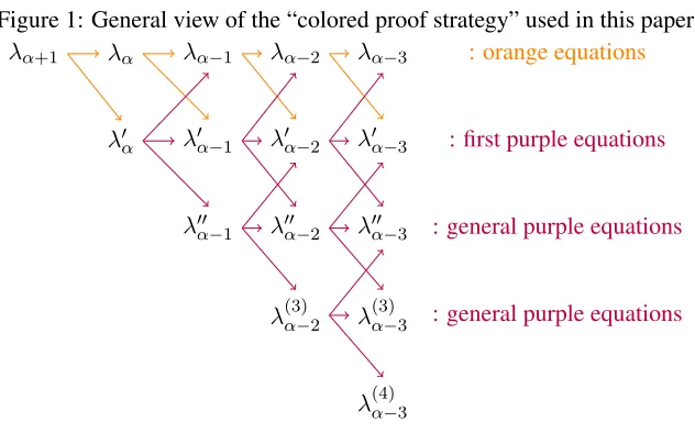
Figure 1: General view of the “colored proof strategy” used in this paper
λα+1 λα λα−1 λα−2 λα−3 : orange equations
λ0α λ0α−1 λ0α−2 λ0α−3 : first purple equations
λ00α−1 λ00α−2 λ00α−3 : general purple equations
λ(3)α−2 λ(3)α−3 : general purple equations
λ(4)α−3
2. We get an equation (called the “first purple equation”) that evaluatesλ0αfromλα−1,λ0α−1 andλ00α−1
(where inλ00α−1we have introduced two extra and independent affine equations from theλα−1
condi-tions). It is sometimes interesting (since it sometimes simplifies the analysis) to introduce a constant
ψin the affine equationsX.
3. We get the equations (called “all purple equations”) that evaluateλ(αd)fromλ(d
−1)
α−1 ,λ (d)
α−1, andλ (d+1)
α−1 ,
(where inλ(αd−1) , we have introduceddextra and independent affine equations from the λα−1
equa-tions).
4. Now, from these evaluations we are able to compare λα+1
λα with
Uα+1
Uα and thereforeλαfromUα. This can be done either with the constant ψ (by looking for the possible deviation) or withψ = 0 (by evaluatingλα).
We have seen that in order to evaluate preciselyλα+1 fromλαwe need to evaluateλ0αfromλα. More
precisely, we have seen that only one term inλ0αwas dominant: the term that we denotedλ0α(4)with 4 indices
(typicalX:f1⊕g2⊕h3 =f4⊕g4⊕h4).
Similarly, when we want to evaluate precisely λ0α, we have seen a formula (“first purple equation”) that givesλ0αfromλα−1,λ0α−1andλ00α−1. In this formula 2 terms inλ0α−1 will be dominant (withXwith 4 or 6
indices) and one term inλ00α−1will be dominant (withXY with 7 indices). This process will continue, with
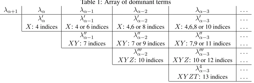
more precise evaluation at each level. The process, and the dominant terms that appear are shown in the array below. The generalization of the “first purple equation” is the “general purple equation” that evaluate(for any integerd)λdα+1+1fromλdα,λαd+1andλdα+2. (This shown for example with the arrow in Table 1 forλ00α−2).
In this figure we see that for the termλdα−iwe need at most(3i+ 4)−(i+ 1−d)indices= 2i+d+ 3
Table 1: Array of dominant terms
λα+1 λα λα−1 λα−2 λα−3 . . .
λ0α λ0α−1 λ0α−2 λ0α−3 . . .
X:4 indices X:4 or 6 indices X:4,6 or 8 indices X:4,6,8 or 10 indices . . . λ00α−1 λ00α−2 λ00α−3 . . .
XY:7 indices XY:7 or 9 indices XY:7,9 or 11 indices . . . λ000α−2 λ000α−3 . . . XY Z:10 indices XY Z:10 or 12 indices . . . λ4α−3 . . . XY ZT:13 indices . . .
12
The first purple equations on general equation
X
The first purple forλ0α(4)(i.e. with equationX:fα+1⊕gα+1⊕hα+1=f1⊕g2⊕h3⊕Ψ, with 4 indices)
was studied in Appendix D and have seen in Section 10 how to simplify the analysis done. Here, in section 12, we will study the first purple equations on more general equationsX. In fact, in section 11, we have seen that in order to prove security whenm2n, first purple equations with 4 indices, 6 indices, 8 indices, 10 indices etc. will appear. Therefore we will need this section 12. Essentially, the analysis with these more general equationXwill be the same as forλ0α(4). LetXbe an affine equation infi,gi,hisuch thatXis not
one of theβi equations. (As before we denote byβ1, . . . , β4α, the4αequations not compatible withλα+1,
i.e.β1 isfα+1=f1. . .,β4αisfα+1⊕gα+1⊕hα+1=fα⊕gα⊕hα.
Without loosing generality (just by changing the name of the indices) we can assume thatXusefα+1
orgα+1 orhα+1. λ0α is the number of sequences(fi, gi, hi),1 ≤i≤ α, that satisfy the conditionλα plus
the equationX.
LetBi0 be the set of solutions that satisfy the conditionsλ0αplus the equationX and conditionβi. We
have
λ0α+1 = 22nλα− | ∪4i=1α Bi0| (1)
Since (as before) 5 equations inβicannot be compatible with the conditionsλα, we obtain from(1):
λ0α+1 = 22nλα−
4α
X
i=1
|Bi0|+X
i<j
|Bi0∩Bj0|
− X
i<j<k
|Bi0∩Bj0 ∩Bk0|+ X
i<j<k<l
|Bi0∩Bj0 ∩B0k∩Bl0| (2)
To analyze(2)in order to get our “first purple equations”, we can proceed directly (as in Appendix D) or by differences betweenXand equationsX⊕ΨwhereΨis constant.
12.1 Method 1: we proceed directly
Letχbe the number of indicesiused in the equationXin the variablesfi,gi,hi.
Theorem 7 (First purple equations)
such that:∀i, 1≤i≤6,0≤i≤1and
λ0α+1 =22n+ (−3−δ1)α.2n+ (3 +δ1)α2+ 2.2n2+ (8−2δ15)α−5
λα
+[(−1 +δ1)α22n+ (3−δ1)α22n−4α3+ (2α2+ 2α)7
+1χ22n−4αχ32n+ 12(χ+ 2)4α2]λ0α
+α4+ (−4χ−12)6α3
λ00α
Proof Theorem 7 can be proved from(2)in a similar way as we did in Appendix D (i.e. by looking for
X+ 1equationsβi,X+ 2equationsβi,X+ 3equationsβi, andX+ 4equationsβi). We do not give the
details here since we can avoid Theorem 7 by looking only for differences betweenΨ6= 0andΨ = 0.
12.2 Method 2: Looking for differences between Equation X and Equation X+ Ψ (“Hσδ
method”)
We want to prove that all the valuesλ0α(or all the “dominant” valuesλ0αas seen in section 11) are very near
λα
2n. For this we can imagine:
1. To evaluate all this valuesλ0α(X)directly: this is what was done with Method 1. 2. To evaluate|λ0α(X)−λ0α(Y)|for any two (dominant) equationsXandY. 3. To evaluate only|λ0α(X)−λ0α(X⊕Ψ)|: this is what will be done here.
From3)we will get2)easily thanks to the “stabilization formula inλ0α(Ψ)”: for all equationXwe have:
X
Ψ∈In
λ0α(X⊕Ψ) =λα
(IfΨ6= 0, this also gives:(2n−1)λ0α(Ψ) +λ0α = λα, since all the valuesλ0α(Ψ)withΨ6= 0are equal).
So we just have to analyze|λ0α(X)−λ0α(X⊕Ψ)|, i.e.|λ0α−λ0α(Ψ)|with simplified notation whereXis fixed. As in section 10 (or Appendix D, equation D6), from(2)we will obtain:
λ0α+1−λ0α+1(Ψ) =δα(X) +A+B
whereδα(X) is the only term not in(λ0α−λ0α(Ψ))or(λ00α−λ00α(Ψ)),A is the terms in(λ0α −λ0α(Ψ))
andB is the terms in(λ00α−λ00α(Ψ)). Sinceα 2n, the coefficients inAare decreasing (i.e. “the part
is quickly vanishing”). The term inBwill be analyzed in the next section (in a similar way). Finally, when
α 2n, the terms inδα(X)will be quickly dominant (ifδα(X) 6= 0). Forλ
0(4)
α we have seen (cf section
10 or Appendix D) that
δα(λ
0(4)
α ) =−λα+ 3(α−1)λ
0∗(2)
α (Ψ) + (α−3)λ
0(4)
α + 3λ
0(3)
α −(3α2−3α−6)λ
00∗
α (Ψ).
Let evaluate the other mainδα in the same way. For all dominant equation X (cf section 10) with ≥ 6
variables, we have:δα(X) = 0(since with 1,2,3 or 4 equations inβiwe cannot obtain0 = Ψor an equation
13
The second purple equations
Let X and Y be two independent and compatible affine equations in fi, gi, hi, 1 ≤ i ≤ α. Here by
“compatible” we mean that fromX, Y orX ⊕Y we cannot obtain an equation fi = fj, orgi = gj, or
hi =hj, orfi⊕gi⊕hi=fj⊕gj⊕hk, or0 = ΨwithΨa constant6= 0withi6=j.
λ00αis the number of sequences(fi, gi, hi),1≤i≤α,fi ∈In, gi ∈In, hi ∈Inthat satisfy the conditions
λαplus the equationsXandY. We will proceed in a way similar to section 12 in order to get an induction
formula that givesλ00α+1 fromλ00α, λ0α andλ000α (we will also denote λ000α = λ3α). As before, we denote by
β1, β2, . . . , β4α, the4αequations not compatible withλα+1. LetBi0 be the set of solutions that satisfy the
conditionsλ00αplus the equationsXandY and the conditionβi. Without losing generality (by the symmetry
of the hypotheses inf, g, handf ⊕g⊕h) we can assume thatXis of this type:
X:gα+1 =⊕of terms of indices≤αinfi, gi, hi.
We have:
λ00α+1 = 22nλ0α− | ∪4i=1α Bi0| (1)
Since (as before) 5 equations inβicannot be compatible, we obtain from(1):
λ00α = 22nλ0α−
4α
X
i=1
|B0i|+X
i<j
|B0i∩Bj0|
− X
i<j<k
|Bi0∩Bj0 ∩Bk0|+ X
i<j<k<l
|Bi0∩Bj0 ∩B0k∩Bl0| (2)
We want to prove that all the valuesλ00α(or all the “dominant” valuesλ00αas seen in section 11) are very near
λα
22n.
For this we can imagine:
1. To evaluateλ00α(X, Y) directly. This can be obtained from Theorem 8 or Theorem 9 of next section 14, but we can avoid these theorems as we will see now.
2. To evaluate|λ00α(X, Y)−λ00α(Z, T)|for any two couples of (dominant) equations(X, Y)and(Z, T). 3. To evaluate|λ00α(X, Y)−λα00(X, T)|and to use|λ00α(X, Y)−λ00α(Z, T)| ≤ |λ00α(X, Y)−λ00α(X, T)|+
|λ00α(X, T)−λ00α(Z, T)|.
4. To evaluate only|λ00α(X, Y)−λα00(X⊕Ψ, Y)|, whereΨis a constant: this is what we will do here. From4)we will get3)(and then2)) easily thanks to the “Stabilization formula inλ00α(Ψ)”: for all equation
Xwe haveP
Ψ∈Inλ
00
α(X⊕Ψ, Y) =λ0α(Y), and from section 12 we know thatλ0α(Y)is near λ2αn. So if we can prove that for given equationsXandY, we have:∀Ψ∈In,|λ00α(X, Y)−λ00α(X⊕Ψ, Y)|is small, then
we getλ00α(X, Y)is nearλ0α(Y), i.e. near λα
22n. As in section 12, from(2), we will obtain:
λ00α+1(X, Y)−λ00α+1(X⊕Ψ, Y) =δα(X, Y) +A+B
whereA is the term in(λ00α −λ00α(Ψ)),B is the term in(λ000α −λ000α(Ψ)), and δα(X, Y)are the terms not
inAorB. Whenα 2n, from(2)we will get that the terms inδα(X, Y)will be quickly dominant (if
14
The general purple equations
Notations
Letαandβbe two integers. We writeλdα(X1, X−2, . . . , Xd), or simplyλdαfor simplicity, the number of
sequences(fi, gi, hi),1≤i≤α,fi∈In,gi ∈In,hi∈Insuch that:
1. Thefi are pairwise distinct,1≤i≤α.
2. Thegiare pairwise distinct,1≤i≤α.
3. Thehiare pairwise distinct,1≤i≤α.
4. Thefi⊕gi⊕hiare pairwise distinct,1≤i≤α.
5. We have dindependent and compatible affine equations X1, X2, . . . , Xd in the variables fi, gi, hi,
1≤i≤α. Here by “compatible” we mean that by linearity fromX1, X2, . . . , Xd, we cannot obtain
an equationfi = fj, orgi = gj, orhi = hj, orfi ⊕gi⊕hi = fj ⊕gj ⊕hj, or0 = ψwithψ a
constant6= 0, withi6=j.
Thereforeλdαis the number of sequences that satisfy the conditionsλαplus thedequationsX1, X2, . . . , Xd.
By definition, we will say thatλdαis “strong” when all these equationsXk,1 ≤k ≤dcan be written like
this:
fk(orgk orhkorfk⊕gk⊕hk)=⊕of terms of indices≤k−1infi, gi, hi⊕ψ, whereψis a constant
ofIn. (We needψ= 0for our final results, but it is sometimes useful in some proofs to obtain some results
withψ6= 0as well). Remark.
λdαis a simple notation forλdα(X1, X2, . . . , Xd), i.e. the valuesλdαgenerally depend onX1, X2, . . . , Xd.
However, as we will see, all these valuesλdαare often very near. Notation:χ
We will denote byχthe number of indicesiused in thedequationsX1, X2, . . . , Xdin the variablesfi,gi,
hi.
Remark.
This valueχ will help us to evaluate the number of new indices in new equations. Often in our systems we will haveχ α (typically we can haveα 2n andχ n). This value will help us to evaluate the number of new indices in new equations, and therefore when the new systems will be strong.
We will proceed like in section 12 in order to get an induction formula that givesλdα+1+1fromλdα,λdα+1
andλd+2
α As before, we denote byβ1, β2, . . . , β4α, the 4α equations not compatible withλα+1: i.e. β1 :
fα+1 =f1, β2:fα+1=f2, . . . , β4α :fα+1⊕gα+1⊕hα+1 =fα⊕gα⊕hα. LetB0ibe the set of solutions
that satisfy the conditionsλdα plus the equationsX1, X2, . . . , Xd+1 and the conditionβi. We denote byX
the equationXd+1. Without losing generality (by the symmetry of the hypotheses inf, g, handf ⊕g⊕h)
we can assume thatXis of this type:
X:gα+1 =⊕of terms of indices≤αinfi, gi, hi.
We have:
Since (as before) 5 equations in βi cannot be compatible (because then at least 2 comes fromf, g, h or
f⊕g⊕hand therefore are not compatible with the conditionsλα), we obtain from(1):
λdα+1 = 22nλdα−
4α
X
i=1
|Bi0|+X
i<j
|Bi0∩B0j|
− X
i<j<k
|Bi0∩Bj0 ∩Bk0|+ X
i<j<k<l
|Bi0∩Bj0 ∩B0k∩Bl0| (2)
Theorem 8 (“General purple equations on strong”λdα; i.e. onΛdα)
There are some real values1,2,3,4, such that∀i∈ {1,2,3,4}, 0≤i≤1, and:
Λdα+1+1= 22nΛdα−3α.2nΛdα−22n(α−χ)Λαd+1−22nχλdα+1
+3α2Λdα+ 2α(α−χ)2nΛdα+1+ (3αχ).2nλdα+1 −4(α−χ−2)3Λdα+1−(4α3−4(α−χ−2)3−1χ3)λdα+1
−1χ3λdα+2(12αχ2)λdα+1
+(α−χ−3)4Λαd+2+ (α4−(α−χ−3)4−3α(χ3+ 1)−α(χ3+ 5))λdα+2
+3α(χ3+ 1)λdα+1−4(4χ2α2+ 4α)λdα+2
Proof Theorem 8 can be proven in a similar way as we did in Appendix D. However, we do not give the details here since we can avoid this Theorem 8 by using constantsΨ6= 0and looking for differences. Theorem 9 (“General purple equations on usualλdα”)
There are some real values1,2,3,4,5,6, such that∀i∈ {1,2,3,4,5,6}, 0≤i ≤1, and:
λdα+1+1= 22nλdα
−3α·2nλdα−22nαλαd+1+1·χ·22nλdα+1
+3α2λdα+ 3α2·2nλαd+1−2·3χα·2nλdα+1
−(4α3−3χ3)λdα+1−3χ3λdα+4(12αχ2)λdα+1
+(α4−5·α(χ3+ 1))λdα+2
+5·α·(χ3+ 1)λdα+1−6(6χ2α2+α3χ+ 4α)λdα+2
Proof of Theorem 9 Theorem 9 can be proven in a similar way as we did in Appendix D. However, we do not give the give the details here since we can avoid this Theorem 9 by using constantsΨ6= 0and looking for differences.
15
Our security results
Theorem 10
Advm ≤2
hmY−1
α=1
[1 + α(1 +σ(1)) 23n(1− α
2n)4
]−1i1/3
Proof This comes immediately from Theorem 4 and the fact that we have seen in Part III. that
(4)α ≤ −1
22n(1 +σ(1)) (1)
and that the term inα3(3)α andα2(2)α , even if they are≥0are in absolute value smaller than the absolute
value of the term inα4(4)α . Moreover, 2α3n + α
4
24n
(4)
α = 2α3n(1 +σ(1))from(1). Theorem 11 Ifm2n, then
Advm ≤2
m2/3
2n +σ(
m2/3
2n )
Proof Whenm2nTheorem 15.1 gives
Advm ≤2
h
(1 +m(1 +σ(1)) 23n )
m−1i1/3
Advm ≤2
m2(1 +σ(1))
23n ) m1/3
Advm ≤2
m2/3
2n +σ(
m2/3
2n )
Part IV
Variants and Conclusion
16
A simple variant of the schemes with only one permutation
Instead ofG=f1⊕f2, f1, f2 ∈RBn, we can studyG0(x) =f(xk0)⊕f(xk1), withf ∈RBnandx∈In−1.
This variant was already introduced in [2] and it is for this that in [2] p.9 the security in 2mn +O(n) 2mn
3/2
is presented. In fact, from a theoretical point of view, this variantG0is very similar toG, and it is possible to prove that our analysis can be modified to obtain a similar proof of security forG0. In [12], I also studied this problem (with standard coefficientHtechnique, notHσtechniques).
17
A simple property about the Xor of two permutations and a new
conjec-ture
I have conjectured this property:
∀f ∈Fn, if
M
x∈In
f(x) = 0, then∃(g, h)∈Bn2, such thatf =g⊕h.
A new conjecture.However I conjecture a stronger property. Conjecture:
∀f ∈Fn, if
M
x∈In
f(x) = 0, then the numberHof (g, h)∈Bn2,
such thatf =g⊕hsatisfiesH ≥ |Bn|
2
2n2n .
Variant: I also conjecture that this property is true in any group, not only with Xor. In [16] and [10], we give some results about this conjecture.
Remark: in this paper, I have proved weaker results involving m equations with m O(2n) (or
m ≤2n−237n) instead of all the2nequations. These weaker results were sufficient for the cryptographic
security wanted.
18
Conclusion
The results in this paper improve our understanding of the PRF-security of the Xor of two random permu-tations. More precisely in this paper we have proved that the Adaptive Chosen Plaintext security for this problem is in O(2n), and we have obtained an explicit O function. These results belong to the field of finding security proofs for cryptographic designs above the “birthday bound”. (In [1, 8, 11], some results “above the birthday bound” on completely different cryptographic designs are also given). Since building PRF from PRP has many practical applications,we believe that these results are of real interest both from a theoretical point of view and a practical point of view. Our proofs need a few pages, so are a bit hard to read, but the results obtained are very easy to use and the mathematics used are elementary (essentially combinatorial and induction arguments). Moreover, we have proved (in Section 5) that this cryptographic problem of security is directly related to a very simple to describe and purely combinatorial problem. We have obtained this transformation by using the “Hσtechnique”, i.e. combining the “coefficient H technique”
of [13, 11] and a specific computation of the standard deviation ofH. (In a way, from a cryptographic point of view, this is maybe the most important result, and all the analysis after Section 5 can be seen as combina-torial mathematics and not cryptography anymore). It is also interesting to notice that in our proof with have proceeded with “necessary and sufficient” conditions, i.e. that theHσ property that we proved is exactly
equivalent to the cryptographic property that we wanted. Moreover, as we have seen, less strong results of security are quickly obtained.
References
[1] William Aiello and Ramarathnam Venkatesan. Foiling Birthday Attacks in Length-Doubling Trans-formations - Benes: A Non-Reversible Alternative to Feistel. In Ueli M. Maurer, editor,Advances in Cryptology – EUROCRYPT ’96, volume 1070 ofLecture Notes in Computer Science, pages 307–320. Springer-Verlag, 1996.