Modeling Attacks on Physical Unclonable Functions

(1)

Modeling Attacks on Physical Unclonable Functions

Ulrich Rührmair

Computer Science Departm.

TU München 80333 München, Germany

Frank Sehnke

Jan Sölter

Computer Science Departm. TU München

80333 München, Germany

Gideon Dror

The Academic College of Tel-Aviv-Jaffa Tel-Aviv 61083, Israel

Srinivas Devadas

Department of EECS

MIT

Cambrige, MA, USA

Jürgen Schmidhuber

ABSTRACT

We show in this paper how several proposed Physical Un-clonable Functions (PUFs) can be broken by numerical mod-eling attacks. Given a set of challenge-response pairs (CRPs) of a PUF, our attacks construct a computer algorithm which behaves indistinguishably from the original PUF on almost all CRPs. This algorithm can subsequently impersonate the PUF, and can be cloned and distributed arbitrarily. This breaks the security of essentially all applications and proto-cols that are based on the respective PUF.

The PUFs we attacked successfully include standard Arbiter PUFs and Ring Oscillator PUFs of arbitrary sizes, and XOR Arbiter PUFs, Lightweight Secure PUFs, and Feed-Forward Arbiter PUFs of up to a given size and complexity. Our attacks are based upon various machine learning techniques, including Logistic Regression and Evolution Strategies. Our work will be useful to PUF designers and attackers alike.

Keywords

Physical Unclonable Functions, Machine Learning, Crypt-analysis, Physical Cryptography

1. INTRODUCTION

1.1 Motivation and Background

Electronic devices are now pervasive in our everyday life. They are an accessible target for adversaries, which raises a host of security and privacy issues. Classical cryptography offers several measures against these problems, but they all rest on the concept of a secret binary key. Classical cryp-tography presupposes that the devices can contain a piece of information that is, and remains, unknown to the adversary. Unfortunately, it can be difficult to uphold this requirement in practice: Physical attacks such as invasive, semi-invasive,

or side-channel attacks, as well as software attacks like API-attacks and viruses, can lead to key exposure and full secu-rity breaks. The fact that the devices should be inexpensive, mobile, and cross-linked obviously aggravates the problem.

The described situation was one motivation that led to the development of Physical Unclonable Functions (PUFs). A PUF is a (partly) disordered physical systemS that can be challenged with so-called external stimuli or challengesCi,

upon which it reacts with corresponding responses termed RCi. Contrary to standard digital systems, a PUF’s

re-sponses shall depend on the nanoscale structural disorder present in the PUF. This disorder cannot be cloned or re-produced exactly, not even by its original manufacturer, and is unique to each PUF. Assuming the stability of the PUF’s responses, any PUFShence implements an individual func-tion FS that maps challenges Ci to responses RCi of the

PUF.

Due to its complex and disordered structure, a PUF can avoid some of the shortcomings associated with digital keys. It is usually harder to read out, predict, or derive its re-sponses than to obtain the values of digital keys stored in non-volatile memory. This fact has been exploited for vari-ous PUF-based security protocols. Prominent examples in-cluding schemes for identification and authentication [1], key exchange or digital rights management purposes [2].

1.2 Strong PUFs, Controlled PUFs, and Weak

PUFs

There are several subtypes of PUFs, each with its own ap-plications and security features. Three major types, which must explicitly be distinguished in this paper, are Strong PUFs[1, 3, 4] 1_,_{Controlled PUFs}_{[2], and}_{Weak PUFs}_[4], initially termedPhysically Obfuscated Keys (POKs)[5].

1.2.1 Strong PUFs

Strong PUFs are disordered physical systems with a complex challenge-response behavior and very many possible chal-lenges. Their security features are: (i) It must be impossible to physically clone a Strong PUF, i.e., to fabricate a

(2)

ond system which behaves indistinguishably from the origi-nal PUF in its challenge-response behavior. This restriction shall hold even for the original manufacturer of the PUF. (ii) A complete determination/measurement of all challenge-response pairs (CRPs) within a limited time frame (such as several days or even weeks) must be impossible, even if one can challenge the PUF freely and has unrestricted access to its responses. This property is usually met by the large num-ber of possible challenges and the finite read-out speed of a Strong PUF. (iii) It must be difficult to numerically predict the response RC of a Strong PUF to a randomly selected

challengeC, even if many other CRPs are known.

Typical applications of Strong PUFs are key establishment [1, 7], identification [1] and authentication [3], where they can achieve secure protocols without the usual, standard computational assumptions. The currently known electrical, circuit-based candidates for Strong PUFs are described in [8, 9, 10, 11, 12].

1.2.2 Controlled PUFs

A Controlled PUF as described in [2] uses a Strong PUF as a building block, but adds control logic that surrounds the PUF. The logic prevents challenges from being applied freely to the PUF, and hinders direct read-out of its responses. This logic can be used to thwart modeling attacks. However, if the outputs of the embedded Strong PUF can be directly probed, then it may be possible to model the Strong PUF and break the Controlled PUF protocol.

1.2.3 Weak PUFs

Weak PUFs, finally, may have very few challenges — in the extreme case just one, fixed challenge. Their response(s) RCi are used to derive a standard secret key, which is

sub-sequently processed by the embedding system in the usual fashion, e.g. as a secret input for some cryptoscheme. Con-trary to Strong PUFs, the responses of a Weak PUF are never meant to be given directly to the outside world.

Weak PUFs essentially are a special form of non-volatile key storage. Their advantage is that they may be harder to read out invasively than non-volatile memory like EEP-ROM. Typical examples include the SRAM PUF [4], But-terfly PUF [13] and Coating PUF [14]. Integrated Strong PUFs have been suggested to build Weak PUFs or Physi-cally Obfuscated Keys (POKs), in which case only a small subset of all possible challenges is used [5, 8].

1.3 Numerical Modeling Attacks on PUFs

Numerical modeling attacks on PUFs presume that an ad-versary Eve has collected a subset of all CRPs of the PUF, and tries to derive a numerical model from this data, i.e., a computer algorithm which correctly predicts the PUF’s responses to arbitrary challenges with high probability. If successful, this breaks the security of the PUF and of any protocols built on it. It is known from earlier work that ma-chine learning (ML) techniques are a natural and powerful tool for such modeling attacks [5] [15] [16] [17]. How the re-quired CRPs can be collected depends on the type of PUF under attack.

Strong PUFs.

Strong PUFs usually have no protection me-chanisms that prevent Eve from challenging them and read-ing out their responses [1, 8, 9, 10, 11, 12]. Most electrical Strong PUFs operate at high frequencies (e.g., 100 MHz [11]), whence even short access periods enable the read-out of many CRPs. Two other potential CRP sources are sim-ple protocol eavesdropping, for examsim-ple on standard Strong PUF-based identification protocols, where the CRPs are sent in the clear [1], or virus attacks on the PUF-embedding hard-ware.

Controlled PUFs.

For any adversary that is restricted to non-invasive CRP measurement, modeling attacks can be successfully disabled if one uses a secure one-way hash over the outputs of the PUF to create a Controlled PUF. We note that this requires error correction of the PUF outputs which are inherently noisy [2]. Successful application of our tech-niques only becomes possible if Eve can probe the internal, digital response signals of the underlying Strong PUF on their way to the control logic. Even though this is a signif-icant assumption, probing digital signals is still easier than measuring continuous analog parameters within the under-lying Strong PUF, for example determining its delay values.

Weak PUFs.

Weak PUFs are only susceptible to model building attacks if a Strong PUF, embedded in some hard-ware system, is used to derive the physically obfuscated key. This method has been suggested in [5, 8]. In this case, the internal digital response signals of the Strong PUF to in-jected challenges have to be probed.

Purely numerical modeling attacks are not relevant forWeak PUFs with just one challenge (such as the Coating PUF, SRAM PUF, or Butterfly PUF). Other strategies could be applied, including invasive, side-channel and virus attacks. For example, probing the output of the SRAM cell prior to storing the value in a register can break the security of the cryptographic protocol that uses these outputs as a key. Weak PUFs also require error correction of the PUF output.

1.4 Our Contributions and Related Work

We describe successful modeling attacks on all known elec-trical candidates for Strong PUFs, including Arbiter PUFs, XOR Arbiter PUFs, Feed-Forward Arbiter PUFs, Light-weight Secure PUFs, and Ring Oscillator PUFs. Our at-tacks work for PUFs of up to a given size and complexity; the prediction rates of our models significantly exceed the known or derived stability of the respective PUFs in silicon in these ranges.

(3)

cannot be raised at will in practical applications. However, the number of stages in the PUFs can be raised without significant effect on instability.

Our results break the security of any Strong PUF-type pro-tocol that is based on one of the broken PUFs. This includes any identification, authentication, key exchange or digital rights management protocols, such as the ones described in [1, 6, 7, 10, 3]. Under the assumptions and attack scenarios described in Section 1.3, our findings also restrict the use of the broken Strong PUF architectures within Controlled PUFs and as Weak PUFs, if we assume that digital values can be probed.

Related Work.

Earlier work, such as [10] [15] [16], described successful ML attacks on standard Arbiter PUFs and on Feed-Forward Arbiter PUFs with one loop. But these ap-proaches did not generalize to Feed-Forward Arbiter PUFs with more than two loops. The XOR Arbiter PUF, Light-weight PUF, Feed-Forward Arbiter PUF with more than two Feed-Forward Loops, and Ring Oscillator PUF have not been cryptanalyzed thus far. No scalability analyses of the required CRPs and computation times had been performed in previous works.

1.5 Organization of the Paper

The paper is organized as follows. We describe the method-ology of our ML experiments in Section 2. In Sections 3 to 7, we present our results for various Strong PUF candi-dates. They deal with Arbiter PUFs, XOR Arbiter PUFs, Lightweight Arbiter PUFs, Feed-Forward Arbiter PUFs and Ring Oscillator PUFs, in sequence. We conclude with a sum-mary and discussion of our results in Section 8.

2. METHODOLOGY SECTION

2.1 Employed Machine Learning Methods

2.1.1 Logistic Regression

Logistic Regression (LR) is a well-investigated supervised machine learning framework, which has been described, for example, in [18]. In its application to PUFs with single-bit outputs, each challengeC = b1· · ·bk is assigned a

proba-bilityp(C, t|w~) that it generates a outputt ∈ {−1,1}(for technical reasons, one makes the convention thatt∈ {−1,1}

instead of{0,1}). The vectorw~thereby encodes the relevant internal parameters, for example the particular runtime de-lays, of the individual PUF. The probability is given by the logistic sigmoid acting on a functionf(w~) parametrized by the vectorw~ asp(C, t|w~) =σ(tf) = (1 +e−tf₎−1_{. Thereby} f determines throughf = 0 a decision boundary of equal output probabilities. For a given training setM of CRPs the boundary is positioned by choosing the parameter vector ~

win such a way that the likelihood of observing this set is maximal, respectively the negative log-likelihood is minimal:

ˆ ~

w=argminw~l(M, ~w) =argminw~ X

(C, t)∈ M

−ln(σ(tf(w, C~ )))

(1) As there is no analytical solution to determine the optimal parameter vector ˆw~, it has to be optimized iteratively, e.g.,

using the gradient information

∇l(M, ~w) = X (C, t)∈ M

t(σ(tf(w, C~ ))−1)∇f(w, C~ ) (2)

From the different optimization methods which we tested in our ML experiments (standard gradient descent, iterative reweighted least squares, RProp [18] [19]), RProp gradient descent performed best. need not be (approximately) lin-early separable in feature space, as is required for successful application of SVMs, but merely differentiable.

In our ML experiments, we used an implementation of LR with RProp programmed in our group, which has been put online under [20]. The iteration is continued until we reach a point of convergence, i.e., until the averaged prediction rate of two consecutive blocks of five consecutive iterations does not increase anymore for the first time. If the reached performance after convergence on the training set is not suf-ficient, the process is started anew. After convergence to a good solution on the training set, the prediction error is evaluated on the test set.

The whole process is similar to training an Artificial Neural Network (ANN) [18]. The model of the PUF resembles the network with the run time delays resembling the weights of an ANN. Similar to ANNs, we found that RProp makes a very big difference in convergence speed and stability of the LR (several XOR-PUFs were only learnable with RProp). But even with RProp the delay set can end up in a region of the search space where no helpful gradient information is available (local minimum). In such a case we encounter the above described situation of converging on a not sufficiently accurate solution and have to restart the process.

2.1.2 Evolution Strategies

Evolution Strategies (ES) [21, 22] belong to an ML subfield known as population-based heuristics. They are inspired by the evolutionary adaptation of a population of individuals to certain environmental conditions. In our case, one indi-vidual in the population is given by a concrete instantiation of the runtime delays in a PUF, i.e., by a concrete instanti-ation of the vectorw~ appearing in Eqns. (1) and (2). The environmental fitness of the individual is determined by how well it (re-)produces the correct CRPs of the target PUF on a fixed training set of CRPs. ES runs through several evolutionary cycles or so-called generations. With a grow-ing number of generations, the challenge-response behavior of the best individuals in the population better and better approximates the target PUF. ES is a randomized method that neither requires an (approximately) linearly separable problem (like Support Vector Machines), nor a differentiable model (such as LR with gradient descent); a merely param-eterizable model suffices. Since all known electrical PUFs are easily parameterizable, ES is a very well suited attack method.

(4)

of the trainings set are used to evaluate an individual’s en-vironmental fitness; instead, only a randomly chosen subset is used for evaluation. If LE was employed, it is indicated in the caption of our tables.

2.2 Employed Computational Resources

We used two hardware systems to carry out our experi-ments: A stand-alone, consumer INTEL Quadcore Q9300 worth less than 1,000 Euros. Experiments run on this sys-tem are marked with the term “HW⋆”. Secondly, a 30-node cluster of AMD Opteron Quadcores, which represents a worth of around 30,000 Euros. Results that were obtained by this hardware are indicated by the term “HW ”. All computation times are calculated for one core of one proces-sor of the corresponding hardware.

2.3 PUF Descriptions and Models

Arbiter PUFs.

Arbiter PUFs (Arb-PUFs) were first intro-duced in [10] [11] [8]. They consist of a sequence ofkstages, for example multiplexers. Two electrical signals race simul-taneously and in parallel through these stages. Their ex-act paths are determined by a sequence ofk external bits b1· · ·bkapplied to the stages, whereby thei-th bit is applied

at thei-th stage. After the last stage, an “arbiter element” consisting of a latch determines whether the upper or lower signal arrived first and correspondingly outputs a zero or a one. The external bits are usually regarded as the challenge C of this PUF, i.e., C = b1· · ·bk, and the output of the

arbiter element is interpreted as their responseR. See [10] [11] [8] for details.

It has become standard to describe the functionality of Arb-PUFs via an additive linear delay model [15] [9] [16]. The overall delays of the signals are modeled as the sum of the delays in the stages. In this model, one can express the final delay difference ∆ between the upper and the lower path in a k-bit Arb-PUF as ∆ = w~T_{Φ, where}_~ _w_~ _and _~_{Φ are of}

dimensionk+1. The parameter vectorw~encodes the delays for the subcomponents in the Arb-PUF stages, whereas the feature vector ~Φ is solely a function of the applied k−bit challengeC [15] [9] [16].

The outputtof the Arb-PUF is then determined by the sign of the propagation delay difference ∆, making the technical convention of saying thatt=−1 when the Arb-PUF output is actually 0, andt= 1 when the Arb-PUF output is 1:

t=sgn(∆) =sgn(w~T~Φ). (3)

Eqn. 3 shows that the vectorw~ viaw~T_{Φ = 0 determines a}_~

separating hyperplane in the space of all feature vectors~Φ. Any challengesC that have their feature vector located on the one side of that plane give responset=−1, those with feature vectors on the other side t= 1. Determination of this hyperplane allows prediction of the PUF.

XOR Arbiter PUFs.

One possibility to strengthen the re-silience of arbiter architectures against machine learning, which has been suggested in [8], is to employ l individual Arb-PUFs in parallel, each withk stages. The same chal-lengeCis applied to all of them, and their individual outputs

ti are XORed in order to produce a global response tXOR.

We denote such an architecture asl-XOR Arb-PUF.

A formal model for the XOR Arb-PUF can be derived as follows. Making the convention ti ∈ {−1,1} as earlier, it

holds thattXOR=Qli=1ti.This leads with equation (3) to

a parametric model of anl-XOR Arb-PUF:

tXOR = l Y

i=1

sgn(w~Ti~Φi) =sgn( l Y

i=1 ~

wTi~Φi) (4)

= sgn(

l O

i=1 ~ wTi

| {z } ~ wX OR

l O

i=1 ~ Φi

| {z } ~

ΦX OR

) =sgn(w~TXORΦ~XOR).(5)

Whereas (4) gives a non-linear decision boundary withl(k+ 1) parameters, (5) defines a linear decision boundary by a separating hyperplanew~XORwhich is of dimension (k+ 1)l.

Lightweight Secure PUFs.

Another type of PUF, which we term Lightweight Secure PUF or Lightweight PUF for short, has been introduced in [9]. It is similar to the XOR Arb-PUF of the last section. At its heart are l individual standard Arb-PUFs arranged in parallel, each withkstages, which produce individual responses/outputsr1, . . . , rl. These

individual outputs are XORed to produce a multi-bit output o1, ..., omof the Lightweight PUF, according to the formula

oj= M

i=1,...,x

r(j+s+i) modl forj= 1, . . . , m. (6)

Thereby the values form(the number of output bits of the Lightweight PUF),x(the number of valuesrjthat influence

each single output bit) ands (the circular shift in choosing thexvaluesrj) are variable design parameters.

Another difference to the XOR Arb-PUFs lies in the l in-puts C1 =b11· · ·b1k, C2 =b12· · ·b2k, . . . , Cl =bl1· · ·blk which

are applied to thelindividual Arb-PUFs. Contrary to XOR Arb-PUFs, it does not hold thatC1 =C2=. . .=Cl=C,

but a more complicated input mapping that derives the in-dividual inputsCifrom the global inputCis applied. This

input mapping constitutes the most significant difference be-tween the Lightweight PUF and the XOR Arb PUF. We refer the reader to [9] for further details.

In order to predict the whole output of the Lightweight PUF, one can apply similar models and ML techniques as in the last section to predict its single output bits oj. While the

probability to predict the full output of course decreases exponentially in the misclassification rate of a single bit, the stability of the full output of the Lightweight PUF also decreases exponentially in the same parameters. It therefore seems fair to attack it in the described manner; in any case, our results challenge the bit security of the Lightweight PUF.

(5)

circuit. Additional arbiter components evaluate these delay differences, and their output bit is fed into said multiplexers in a “feed-forward loop” (FF-loop). The number of loops as well as the starting and end point of the FF-loops are vari-able design parameters. Please note that a FF Arb-PUF withk-bit challengesC=b1· · ·bkandlloops hass=k+l

multiplexers or stages.

The described dependency makes natural architecture mod-els of FF Arb-PUFs no longer differentiable. Consequently, FF Arb-PUFs cannot be attacked generically with ML meth-ods that require linearly separable or differentiable mod-els (like SVMs or LR), even though such modmod-els can be found in special cases, for example for small numbers of non-overlapping loops, etc.

Ring Oscillator PUFs.

Ring Oscillator PUFs (RO-PUFs) were discussed in [8]. They are based on the influence of fabrication variations on the frequency of several, identi-cally designed ring oscillators. While [8] describes the use of Ring Oscillator PUFs in the context of Controlled PUFs and limited-count authentication, it is worth analyzing them as candidate Strong PUFs. A RO-PUF consists ofksuch oscil-lators, each of which has its own, unique frequency caused by manufacturing tolerances. The input of a RO-PUF consists of a tuple (i, j), which selects two of thekoscillators. Their frequencies are compared, and the output of the RO-PUF is “0” if the former oscillates faster than the latter, and “1” else. A ring oscillator can be modeled in a straightforward fashion by a tuple of frequencies (f1, . . . , fk). Its output on

input (i, j) is “0” iffi> fj, and “1” else.

2.4 CRP Generation and Prediction Error

Given a concrete PUF-architecture that should be examined, the challenge-response pairs (CRPs) we used in our ML ex-periments were generated pseudo-randomly in the following fashion: (i) The delay values of the given PUF were chosen randomly according to a standard normal distribution. (ii) A set of challenges was selected uniformly at random from all possible challenges. (iii) The corresponding responses were calculated by use of the delays selected in step (i), and by application of a linear additive delay model [12]. The gen-erated CRPs are subsequently used for training and testing the ML algorithm. 5/6 of the CRPs were used as training set, the rest as test set. For XOR and Lightweight PUFs, a fixed number of 10,000 CRPs were used for testing.

We will use the following definitions throughout the paper: NT rSet is the number of CRPs in the training set. NT eSet

is the number of CRPs in the test set. NCRP is the total

number of employed CRPs, so NCRP =NT rSet+NT eSet.

The prediction error is the ratio of incorrect responses of the trained ML algorithm when evaluated on the test set. In other words, it is the number of incorrect responses of the trained model on the test set divided by number of CRPs in the test set.

3. ARBITER PUFS

3.1 Machine Learning Results

To determine the separating hyperplane w~T_~_{Φ = 0 we}

ap-plied SVMs, LR and ES. LR achieved the best results, which

are shown in Table 1. We chose three different prediction rates as targets: 95% is roughly the environmental stabil-ity of a 64-bit Arbiter PUF when exposed to a temperature variation of 45C and voltage variation of±2% 2. The val-ues 99% and 99.9%, respectively, represent benchmarks for optimized ML results. All figures in Table 1 were obtained by averaging over 5 different training sets. Accuracies were estimated using test sets of 10,000 CRPs.

ML No. of Prediction CRPs Training

Method Stages Rate Time

LR 64

95% 640 0.01 sec

99% 2,555 0.13 sec 99.9% 18,050 0.60 sec

LR 128

95% 1,350 0.06 sec 99% 5,570 0.51 sec 99.9% 39,200 2.10 sec

Table 1: LR on Arb PUFs with 64 and 128 stages.

We used HW ⋆.

3.2 Scalability

We also executed scalability experiments with LR, which are displayed in Fig. 1 and Fig. 2. They show that the relevant parameters – the required number of CRPs and the computational complexity, i.e. number of basic opera-tions – grow both linearly or low-degree polynomially in the misclassification rate ǫand the length k of the Arb PUF. Theoretical considerations (dimension of the feature space, Vapnik-Chervonenkis dimension) suggest that the minimal

number of CRPsNCRP that is necessary to model ak-stage

arbiter with a misclassification rate of ǫ should obey the relation

NCRP = O(k/ǫ). (7)

This was confirmed by our experimental results.

In practical PUF applications, it is essential to know the concrete number of CRPs that may become known before the PUF-security breaks down. Assuming an approximate linear functional dependencyy=ax+cin the double loga-rithmic plot of Fig. 1 with a slope ofa=−1, we obtained the following empirical formula (8). It gives the approximate number of CRPsNCRP that is required to learn ak-stage

arbiter PUF with error rateǫ:

NCRP ≈ 0.5· k+ 1

ǫ (8)

Our experiments also showed that the training time of the ML algorithms, measured in the number of basic operations NBOP, grows slowly. It is determined by the following two

factors: (i) The evaluation of the current model’s likelihood (1) and its gradient (2), and (ii) the number of iterations of the optimization procedure before convergence occurs (see section 2.1.1). The former is both a sum over a function of the feature vectorsΦ for all~ NCRP, and therefore has

com-plexity O(k·NCRP). On the basis of the data shown in

(6)

Figure 1: Double logarithmic plot of

misclassifica-tion rateǫon the ratio of training CRPs NT rSet and

dim(Φ) =k+ 1.

Figure 2: No. of iterations of the LR algorithm un-til “convergence” occurs (see section 2), plotted in

dependence of the training set sizeNT rSet.

Figure 2, we may further estimate that the numbers of iter-ations increases proportional to the logarithm of the number of CRPsNCRP. Together, this yields an overall complexity

of

NBOP = O

k2 ǫ ·log

k ǫ

. (9)

4. XOR ARBITER PUFS

4.1 Machine Learning Results

In the application of SVMs and ES to XOR Arb-PUFs, we were able to break small instances, for example XOR Arb-PUFs with 2 or 3 XORs and 64 stages. LR significantly outperformed the other two methods. The key observation is that instead of determining the linear decision boundary (5), one can also specify the non-linear boundary (4). This is done by setting the LR decision boundaryf=Ql_i₌₁w~Ti~Φi.

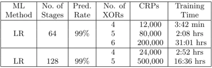
The results are displayed in Table 2.

4.2 Performance on Error-Inflicted CRPs

ML No. of Pred. No. of CRPs Training

Method Stages Rate XORs Time

LR 64 99%

4 12,000 3:42 min 5 80,000 2:08 hrs 6 200,000 31:01 hrs

LR 128 99%

4 24,000 2:52 hrs 5 500,000 16:36 hrs

Table 2: LR on XOR Arbiter PUFs. Training times

are averaged over different PUF-instances. HW⋆.

The CRPs used in Section 4.1 have been generated pseudo-randomly via an additive, linear delay model of the PUF. This deviates from reality in two aspects: First of all, the CRPs obtained from real PUFs are subject to noise and random errors. Secondly, the linear model matches the phe-nomena on a real circuit very closely [15], but not perfectly. This leads to a deviation of any real system from the linear model on a small percentage of all CRPs.

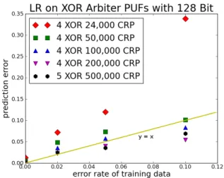
In order to mimic this situation, we investigated the ML performance if a small error had been injected artificially into the training sets. A given percentage of responses in the training set were chosen randomly, and their bit values were flipped. Afterwards, the ML performance on the unaltered, error-free test sets was evaluated. The results are displayed in Tables 3 and 4. They show that LR can cope very well with errors, provided that around 3 to 4 times more CRPs are used. The required convergence times on error inflicted training sets did not change substantially compared to error free training sets of the same sizes.

CRPs Percentage of error afflicted CRPs

(×103) 0% 2% 5% 10%

24

Best Pred. 98.76 92.83 88.05 -Aver. Pred. 98.62 91.37 88.05 -Trial Succ. 0.6% 0.8% 0.2% 0.0%

Instances 40.0% 25.0% 5.0% 0.0%

50

Best Pred. 99.49 95.17 92.67 89.89 Aver. Pred. 99.37 94.39 91.62 88.20 Trial Succ. 12.4% 13.9% 10.0% 4.6% Instances 100.0% 62.5% 50.0% 20.0%

200

Best 99.88 97.74 96.01 94.61

Aver. Pred. 99.78 97.34 95.69 93.75 Trial Succ. 100.0% 87.0% 87.0% 71.4%

Instances 100.0% 100.0% 100.0% 100.0%

Table 3: LR on 128 bit, 4 XOR Arb PUFs with dif-ferent amounts of error in the training set. We show the best and average of 40 independent trials, and the percentage of trials and instances that converged

to a sufficient optimum. We used HW .

4.3 Scalability

(7)

(x103) 0% 2% 5% 10%

500

Best Pred. 99.90 97.55 96.48 93.12 Aver. Pred. 99.84 97.33 95.84 93.12 Trial Succ. 7.0% 2.9% 0.9% 0.7% Instances 20.0% 20.0% 10.0% 5.0%

Table 4: LR on 128 Bit, 5 XOR Arb PUFs with different amounts of error in the training set. Rest

as in the caption of Table 3. HW.

Figure 3: Graphical illustration of the effect of error on LR in the training set, with chosen data points

from Tables 3 and 4. HW.

Arb-PUFsl):

NCRP ∼ (k+ 1)·l

ǫ . (10)

But, in contrast to (standard) Arb-PUFs, optimizing the non-linear decision boundary (4) on the training set now is a non-convex problem, so that the LR algorithm is not guaranteed to find the global optimum in its first trial. It needs to be iteratively restartedNtrialtimes. Ntrialthereby

can be expected to not only depend onk andl, but also on the sizeNT rSetof the employed training set.

As it is argued in greater detail in [17], the success rate of obtaining the global optimum is indeed determined by the ratio of dimensions gradient information exists for (∝NCRP

as the gradient is a linear combination of the feature vector) and the dimensiondΦin which the problem is linear separa-ble. The dimensiondΦis thereby the number of independent dimensions ofΦ~XOR.

As the tensor product of l vectors consists of all possible products between their vector components, the independent dimensions are given by the number of different products Φi1

1 ·Φ

i₂

2 ·. . .Φ

il

l for i1, i2, . . . , ik ∈ {1,2, . . . , k+ 1}. For

XOR Arb-PUFs, we have an equal mapping Φij= Φij′. Since

a repetition of one component does not affect the product regardless of its value Φr_·_Φr₌_±₁_{· ±}_{1 = 1, the uniqueness}

of al-tuple with a repetition is solely determined by its un-repeated components. Therefore the number of independent dimensions is given as the number ofl-tuple without repe-tition, (l−2)-tuple without repetition (corresponding to all

100 ₁₀1 ₁₀2 ₁₀3

CRPs/(k+1)l 10-4

10-3 10-2 10-1 100

prediction error

y = 0.577 * x^(-1.007)

LR on XOR Arbiter PUFs

64 Bit, 2 XOR 64 Bit, 3 XOR 64 Bit, 4 XOR 128 Bit, 2 XOR 128 Bit, 3 XOR

Figure 4: Double logarithmic plot of misclassification

rateǫon the ratio of training CRPsNT rSet and

prob-lem size dim(Φ) = (k+ 1)·l. We used HW.

10-3 ₁₀-2 ₁₀-1

CRPs/dΦ

10-3 10-2 10-1 100

sucess rate

LR on XOR Arbiter PUFs

64 Bit, 4 XOR 64 Bit, 5 XOR 64 Bit, 6 XOR 128 Bit, 3 XOR 128 Bit, 4 XOR 128 Bit, 5 XOR

Figure 5: Average rate of success of the LR algorithm

plotted in dependence of the ratiodΦ(see Eqn. (11))

to NCRP. We used HW.

distinguishablel-tuple with 1 repetition), (l−4)-tuple with-out repetition (corresponding to all distinguishable l-tuple with 2 repetitions), etc.

The number of unique productsdΦis therefore given as:

dΦ= k+ 1

l !

+ k+ 1 l−2 !

+ k+ 1 l−4 !

+. . .≈(k+ 1)

l l! . (11)

All in all, this leads to a numberNtrialof the expected

num-ber of restarts of the optimization procedure until a decision boundary is obtained, of

Ntrial=O

₍_k_{+ 1)}l

NT rSet·l!

. (12)

This equation governs the computational complexity of our approach. One trial has the computational complexity of

(8)

As explained above,NT rSetis the size of the employed

train-ing set. Although a (minimal) traintrain-ing set sizeNT rSet on

the order of (k+ 1)·lis sufficient to learn the XOR Arb-PUF with prediction rate 99%, Eqn. 12 indicates a positive trade-off betweenNtrial andNT rSet. Due to Eqn. 13 it

ap-pears however that the overall complexity is independent of NT rSet. Still, NT rSet needs to be large enough for the

process to converge at all. Due to the constant factors in-volved we find in practice that there is an optimalNT rSet

that optimizes runtime. This optimum lies near the point that Eqn. 11 gives an approximate number of trials of 1.

5. LIGHTWEIGHT SECURE PUFS

5.1 Machine Learning Results

In order to test the influence of the specific input mapping of the Lightweight PUF on its machine-learnability (see Sec. 2.3), we examined architectures with the following parame-ters: Variablel,m= 1,x=l, and arbitrarys.We focused on LR right from the start, since this method was best in class for XOR Arb-PUFs, and obtained the results shown in Ta-ble 5. The specific design of the Lightweight PUF improves its ML resilience by a notable quantitative factor, especially with respect to the training times.

No. of Pred. No. of CRPs Training

Stages Rate XORs Time

64 99%

3 6,000 8.9 sec

4 12,000 1:28 hrs 5 300,000 13:06 hrs

128 99%

3 15,000 40 sec

4 500,000 59:42 min

5 106 267 days

Table 5: LR on Lightweight PUFs. Prediction rate

refers to single output bits. Training times were

averaged over different PUF instances. HW⋆.

5.2 Scalability

Some theoretical consideration [17] shows the underlying ML problem for the Lightweight PUF and the XOR Arb PUF are qualitatively identical, and differ only quantitatively. This means that the asymptotic formulas onNCRP and Ntrial

that were given for the XOR Arb PUF (Eqns. 12 and 13 of Sec. 4.3) also hold for the Lightweight PUF.

This was confirmed by our scalability experiments. We also observed in agreement with Sec. 5.1 that the involved con-stants differ: With the same ratioCRP s/dΦthe LR algo-rithm will have a longer runtime for the Lightweight PUF than for the XOR Arb-PUF. For example, while with a train-ing set size of 12,000 for the 64 Bit 4 XOR Arb-PUF on average about 5 trials were sufficient, for the corresponding Lightweight PUF 100 trials were necessary. In principle, this effect can be compensated by using larger training sets.

6. FEED FORWARD ARBITER PUFS

6.1 Machine Learning Results

We experimented with SVMs and LR on FF Arb-PUFs, us-ing different models and input representations, but could

only break special cases with small numbers of non-overlapp-ing FF loops, such as l = 1,2. This is in agreement with earlier results reported in [16].

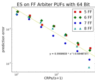
The application of ES finally allowed us to tackle much more complex FF-architectures with up to 8 FF-loops. All loops have equal length, and are distributed regularly over the PUF, with overlapping start- and endpoints of successive loops. Table 6 shows the results we obtained. Please note for comparison that in-silicon implementations of 64-bit FF Arb-PUFs with 7 FF-loops are known to have an environ-mental stability of 90.16% [15].

No. of FF- Pred. Rate CRPs Training

Stages loops Best Run Time

64

6 97.72% 50,000 27:20 hrs 7 97.37% 50,000 27:20 hrs 8 95.46% 50,000 27:20 hrs

Table 6: ES on Feed-Forward Arbiter PUFs. Pre-diction rates are for the best of a total of 40 trials. Training times are for a single trials. We applied

Lazy Evaluation with 2,000 CRPs, and used HW.

6.2 Results on Error-Inflicted CRPs

For the same reasons as in Section 4.2, we evaluated the performance on error-inflicted CRPs with respect to ES and FF Arb PUFs. The results are shown in Table 7 and Fig. 6. ES possess an extremely high tolerance against the inflicted errors; its performance is hardly changed at all.

(×103) 0% 2% 5% 10%

50

Best Pred. 98.29 97.78 98.33 97.68 Aver. Pred. 89.94 88.75 89.09 87.91 Trial Succ. 42.5% 37.5% 35.0% 32.5%

Table 7: ES on 64 bit, 6 FF Arb PUFs with differ-ent levels of error in the training set. The results are the best and average over 40 independent trials. The table also shows the percentage of trials that

converged to 10% or better. We used HW.

6.3 Scalability

We started by empirically investigating the CRP growth as a function of the number of challenge bits, examining archi-tectures of varying bitlength that all have 6 FF-loops. The loops are distributed as described in Section 6.1. The cor-responding results are shown in Figure 7. Every data point corresponds to the averaged prediction error of 10 trials on the same, random PUF-instance, whereby the prediction er-ror for each denotes the difference between the test and the training set. The given number of CRPs is the sum of the sizes of both sets.

(9)

Figure 6: Graphical illustration of the tolerance of ES to errors. We show the best result of 40 inde-pendent trials for varying error levels in the training

set. The results hardly differ. We used HW.

in Figure 8. Each data point shows the averaged prediction error of 10 trials, and the shown numbers of CRPs are again the added sizes of the test and the training set.

In contrast to the former sections 4.3 and 5.2, it is much more difficult to derive reliable scalability formulas from the ES data. Firstly, the structure of ES provides less theoretical footing for formal derivations. Secondly, also an empirical derivation of formulas is intricate, since the inherently ran-dom nature of ES produces a very large variance in the data points. Thirdly, we observed an interesting effect when com-paring the performance of ES vs. SVM/LR on the Arb PUF: While the supervised ML methods SVM and LR showed a linear relationship between the aspired prediction errorǫand the required CRPs even for very smallǫ, ES proved more CRP hungry in these regions, clearly showing a superlin-ear growth. The same effect can be expected for the more complicated FF architectures, meaning that one consistent formula for extreme values ofǫmay be difficult to obtain, at least empirically.

Even though there is a large variation, it is possible to con-clude from the data points in Figs. 7 and 8 that the growth in CRPs is about linear, and that the computation time grows polynomially. Nevertheless, we would like to remain conservative here, and present the upcoming empirical for-mulas only in the status of a conjecture.

The data gathered in our experiments is best explained by assuming qualitative relation of the form

NCRP =O(s/ǫc) (14)

for some constant 0< c <1. Concrete estimation from our data points leads to an approximate formula of the form

NCRP ≈ 9· s+ 1

ǫ3/4 . (15) Thecomputation timerequired by ES is determined by the following factors: (i) The computation of the vector product ~

wT_~_{Φ, which grows linearly with}_s_{. (ii) The evolution applied}

to this product, which is negligible compared to the other

Figure 7: Results of 10 trials per data point with ES for different lengths of FF Arbiter PUFs and the

hyperbola fit. HW.

Figure 8: Results of 10 trials per data point with ES for different numbers of FF-loops and the hyperbola

fit. HW .

steps. (iii) The number of iterations or“generations”in ES until a small misclassification rate is achieved. We conjec-ture that this grows linearly with the number of multiplexers s. (iv) The number of CRPs that are used to evaluate the individuals per iteration. If Eqn. 15 is valid, thenNCRP is

on the order ofO(s/ǫc).

Assuming the correctness of the conjectures made in this derivation, this would lead to a polynomial growth of the computation time in terms of the relevant parametersk, l and s. It could be hypothesized that the number of basic computational operationsNBOP obeys

NBOP =O(s3/ǫc) (16)

(10)

7. RING OSCILLATOR PUFS

7.1 Possible Attacks

There are several strategies to attack a RO-PUF. The most straightforward attempt is a simple read out of all CRPs. This is easy, since there are justk(k−1)/2 =O(k2) CRPs of interest.

If Eve is able to choose the CRPs adaptively, she can employ a standard sorting algorithm to sort the RO-PUF’s frequen-cies (f1, . . . , fk) in ascending order. This strategy

subse-quently allows her to predict all outputs with 100% correct-ness, without knowing the exact frequenciesfi themselves.

The time and CRP complexities of the respective sorting al-gorithms are well known [24]; for example, there are several algorithms with average and even worst case CRP complex-ity of NCRP = O(k·logk). Their running times are also

low-degree polynomial.

The most interesting case for our investigations is when Eve cannot adaptively choose the CRPs she obtains, but still wants to achieve optimal prediction rates. This case occurs in practice whenever Eve obtains her CRPs from protocol eavesdropping, for example. We carried out experiments for this case, in which we applied Quick Sort (QS) to randomly drawn CRPs. The results are shown in Table 8. The esti-mated required number of CRPs is given by

NCRP ≈k(k−1)(1−2ǫ)

2 +ǫ(k−1) , (17)

and the training times are low-degree polynomial. Eqn. 17 quantifies limited-count authentication capabilities of RO-PUFs.

Method No. of Pred. Rate CRPs

Oscill. average

QS

256 99% 99.9% 14,060 28,891

512 99% 99.9% 36,062 103,986 1024 99% 99.9% 83,941 345,834

Table 8: Quick Sort applied to the Ring Oscillator PUF. The given CRPs are averaged over various

tri-als. We used HW.

8. SUMMARY AND DISCUSSION

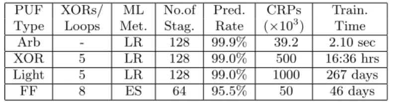
We investigated the resilience of electrical Strong PUFs against modeling attacks. To that end, we applied various ma-chine learning techniques to challenge-response data gener-ated pseudo-randomly via an additive delay model. Some of our main results are summarized in Table 9.

We found that all examined Strong PUF candidates under a given size could be machine learned with success rates above their in-silicon stability. The attacks require a number of CRPs that grows only linearly or log-linearly in the inter-nal parameters of the PUFs, such as their number of stages, XORs, feed-forward loops or ring oscillators. Apart from XOR Arbiter PUFs and Lightweight PUFs (whose training times grew super-polynomially in their number of XORs), the training times of the applied machine learning algo-rithms are low-degree polynomial, too. These results sug-gest that XOR-based architectures are a favorable approach for PUF design. But one observation is that not only the

PUF XORs/ ML No.of Pred. CRPs Train.

Type Loops Met. Stag. Rate (×103) Time

Arb - LR 128 99.9% 39.2 2.10 sec

XOR 5 LR 128 99.0% 500 16:36 hrs

Light 5 LR 128 99.0% 1000 267 days

FF 8 ES 64 95.5% 50 46 days

Table 9: Some of our main results.

machine learning resilience, but also the instability of the XOR-based approaches increases exponentially in the num-ber of XORs l. Therefore, there is a limit on l [25]. On the other hand, the number of stages in the PUFkis a pa-rameter that the PUF-designer can increase to increase the computational effort of the adversary; for a largel, increas-ing k significantly results in a strongly increased effort for the adversary.

Our results prohibit the use of the broken architectures as Strong PUFs or in Strong-PUF based protocols. Under the assumption that digital signals can be probed, they also af-fect the applicability of the cryptanalyzed PUFs as build-ing blocks in Controlled PUFs and Weak PUFs. While we have presented results only on pseudo-random CRP data generated in the additive delay model, experiments with sili-con implementations [15] have shown that the additive delay model achieves high accuracy. We also found that the stabil-ity of our results against random errors in the CRP data is high. This shows that our approach is robust against some inaccuracies in the model and against measurement noise, which is important in the case where CRP data is collected from silicon PUF chips.

Two directions of future work arise from our results. On the side of the PUF designers, avenues to improve the re-silience of delay-based PUFs against modeling attacks must be examined. Possibilities include increasing the length of the PUF, adding nonlinearity (for example, AND and OR gates that correspond to MAX and MIN operators [15]). An-other option is the combination of Feed-Forward and XOR architectures, since they were susceptible only to different ML techniques, respectively. Moving away from delay-based PUFs, by exploitation of the dynamic characteristics of cur-rent and voltage seems promising. The behavior of certain analog circuits (e.g., Cellular Non-linear Networks) is know to be stable, but nevertheless is guided by complex differen-tial equations. Machine learning the output of such a circuit could prove to be difficult.

(11)

9. REFERENCES

[1] R. Pappu, B. Recht, J. Taylor, and N. Gershenfeld. Physical one-way functions.Science, 297(5589):2026, 2002.

[2] Blaise Gassend, Dwaine Clarke, Marten van Dijk, and Srinivas Devadas. Controlled physical random functions. InProceedings of 18th Annual Computer Security Applications Conference, Silver Spring, MD, December 2002.

[3] B. Gassend, D. Clarke, M. Van Dijk, and S. Devadas. Silicon physical random functions. InProceedings of the 9th ACM Conference on Computer and

Communications Security, page 160. ACM, 2002. [4] J. Guajardo, S. Kumar, G.J. Schrijen, and P. Tuyls.

FPGA intrinsic PUFs and their use for IP protection.

Cryptographic Hardware and Embedded Systems-CHES 2007, pages 63–80, 2007.

[5] B.L.P. Gassend.Physical random functions. Msc thesis, MIT, 2003.

[6] R. Pappu.Physical One-Way Functions. Phd thesis, MIT, 2001.

[7] P. Tuyls and B. Skoric. Strong Authentication with PUFs.In: Security, Privacy and Trust in Modern Data Management, M. Petkovic, W. Jonker (Eds.), Springer, 2007.

[8] G.E. Suh and S. Devadas. Physical unclonable functions for device authentication and secret key generation.Proceedings of the 44th annual Design Automation Conference, page 14, 2007.

[9] M. Majzoobi, F. Koushanfar, and M. Potkonjak. Lightweight secure pufs. InProceedings of the 2008 IEEE/ACM International Conference on

Computer-Aided Design, pages 670–673. IEEE Press, 2008.

[10] B. Gassend, D. Lim, D. Clarke, M. Van Dijk, and S. Devadas. Identification and authentication of integrated circuits.Concurrency and Computation: Practice & Experience, 16(11):1077–1098, 2004. [11] J.W. Lee, D. Lim, B. Gassend, G.E. Suh,

M. Van Dijk, and S. Devadas. A technique to build a secret key in integrated circuits for identification and authentication applications. InProceedings of the IEEE VLSI Circuits Symposium, pages 176–179, 2004. [12] D. Lim, J.W. Lee, B. Gassend, G.E. Suh,

M. Van Dijk, and S. Devadas. Extracting secret keys from integrated circuits.IEEE Transactions on Very Large Scale Integration Systems, 13(10):1200, 2005. [13] S.S. Kumar, J. Guajardo, R. Maes, G.J. Schrijen, and

P. Tuyls. Extended abstract: The butterfly PUF protecting IP on every FPGA. InIEEE International Workshop on Hardware-Oriented Security and Trust, 2008. HOST 2008, pages 67–70, 2008.

[14] P. Tuyls, G.J. Schrijen, B. ˇSkori´c, J. van Geloven, N. Verhaegh, and R. Wolters. Read-proof hardware from protective coatings.Cryptographic Hardware and Embedded Systems-CHES 2006, pages 369–383, 2006. [15] Daihyun Lim.Extracting Secret Keys from Integrated

Circuits. Msc thesis, MIT, 2004.

[16] M. Majzoobi, F. Koushanfar, and M. Potkonjak. Testing techniques for hardware security. In

Proceedings of the International Test Conference (ITC), pages 1–10, 2008.

[17] Jan Sölter.Cryptanalysis of Electrical PUFs via Machine Learning Algorithms. Msc thesis, Technische Universität München, 2009.

[18] C.M. Bishop et al.Pattern recognition and machine learning. Springer New York:, 2006.

[19] M. Riedmiller and H. Braun. A direct adaptive method for faster backpropagation learning: The RPROP algorithm. In Proceedings of the IEEE international conference on neural networks, volume 1993, pages 586–591. San Francisco: IEEE, 1993. [20] http://www.pcp.in.tum.de/code/lr.zip.

[21] T. B¨ack.Evolutionary algorithms in theory and practice: evolution strategies, evolutionary

programming, genetic algorithms. Oxford University Press, USA, 1996.

[22] H.P.P. Schwefel.Evolution and Optimum Seeking: The Sixth Generation. John Wiley & Sons, Inc. New York, NY, USA, 1993.

[23] T. Schaul, J. Bayer, D. Wierstra, Y. Sun, M. Felder, F. Sehnke, T. R¨uckstieß, and J. Schmidhuber. PyBrain.Journal of Machine Learning Research, 1:999–1000, 2010.

[24] C.H. Papadimitriou.Computational complexity. John Wiley and Sons Ltd., 2003.

Modeling Attacks on Physical Unclonable Functions