Sufficient Markov Decision Processes.

(1)

ABSTRACT

WANG, LONGSHAOKAN. Sufficient Markov Decision Processes. (Under the direction of Dr. Eric Laber.)

Advances in mobile computing technologies have made it possible to monitor and

apply data-driven interventions across complex systems in real time. Recent and

high-profile examples of data-driven decision making include autonomous vehicles, intelligent

power grids, and precision medicine through mobile health. Markov decision processes

are the primary mathematical model for sequential decision problems with a large or

indefinite time horizon; existing methods for estimation and inference rely critically on

the correctness of this model. Mathematically, this choice of model incurs little loss in

generality as any decision process evolving in discrete time with observable process states,

decisions, and outcomes can be represented as a Markov decision process. However, in

some application domains, e.g., mobile health, choosing a representation of the underlying

decision process that is both Markov and low-dimensional is non-trivial; current practice

is to select a representation using domain expertise. We propose an automated method for

constructing a low-dimensional representation of the original decision process for which:

(P1) the Markov decision process model holds; and (P2) a decision strategy that leads to

maximal mean utility when applied to the low-dimensional representation also leads to

maximal mean utility when applied to population of interest. Our approach uses a novel

deep neural network to define a class of potential process representations and then searches

within this class for the representation of lowest dimension which satisfies (P1) and (P2).

We illustrate the proposed method using a suite of simulation experiments and application

(2)

reduction in Markov decision processes; Chapter 2 describes and illustrates the specific

dimension reduction technique proposed; Chapter 3 relates to Chapter 2 in methodology,

but tackles a different problem in text-based ordinal regression with an application in

(3)

(4)

Sufficient Markov Decision Processes

by

Longshaokan Wang

A dissertation submitted to the Graduate Faculty of North Carolina State University

in partial fulfillment of the requirements for the Degree of

Doctor of Philosophy

Statistics

Raleigh, North Carolina

2018

APPROVED BY:

Dr. Leonard Stefanski Dr. Eric Chi

Dr. Michael Kosorok Dr. David Roberts

Dr. Eric Laber

(5)

DEDICATION

(6)

BIOGRAPHY

Longshaokan Wang was born on October 27, 1990 in Changsha, Hunan, China to parents

Heping Wang and Huanghong Long. After finishing high school in Qingdao, China, he

moved to the United States to pursue higher education. He obtained his bachelors degree

in Honors Mathematics from University of Notre Dame in 2013. Then he joined the Ph.D.

program in Statistics at North Carolina State University where he conducted research in

dimension reduction, reinforcement learning, deep learning, and artificial intelligence

under the guidance of Dr. Eric Laber. He obtained an en-route masters degree in Statistics

(7)

ACKNOWLEDGEMENTS

I would like to thank my committee members for their support and insights. In particular,

I would like to thank my advisor Dr. Eric Laber for providing guidance on my research,

pushing me to realize my potentials, tolerating my shenanigans, and being a good friend.

I would like to thank my parents for their encouragement and understanding on my

studying abroad, as I was only able to come home once a year.

I would like to thank my friends for keeping me sane on my quest for knowledge.

I would like to thank the Laber Lab members for all the enlightening brainstorming

sessions.

I would like to thank Praveen Bodigutla for introducing me to the exciting world of

Natual Language Processing during my internship with Amazon Conversation AI Team.

The experience proved to be very helpful when I worked on the human trafficking detection

project.

I would like to thank Katie Witkiewitz, Yeng Saanchi, and Cara Jones for providing the

(8)

LIST OF TABLES

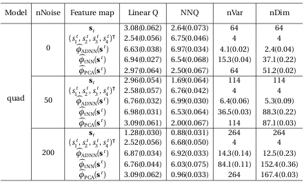
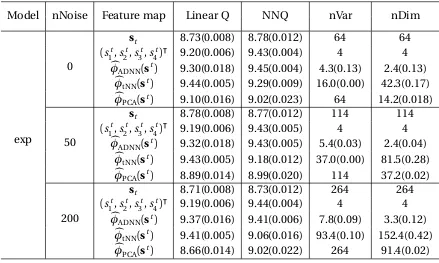
Table 2.1 Comparison of feature map estimators under linear transition across different numbers of noise variables (nNoise) in terms of: marginal mean outcome using Q-learning with linear function approximation (Linear Q); Q-learning with neural network function approximation (NN Q); the number of selected variables (nVar); and the dimension of the feature map (nDim) . . . 27 Table 2.2 Comparison of feature map estimators under quadratic transition . . 28 Table 2.3 Comparison of feature map estimators under exponential transition . 29 Table 2.4 Comparison of feature map estimators in terms of cumulative utility

using DDDQ. Standard errors are included in parentheses. . . 45

Table 3.1 Description and distribution of labels in Trafficking10k. . . 61 Table 3.2 Comparison of our ordinal regression neural network (ORNN) against

(11)

LIST OF FIGURES

Figure 2.1 A basic artificial neural network with 2 hidden layers. . . 18

Figure 2.2 Schematic for alternating deep neural network (ADNN) model. The term “alternating” refers to the estimation algorithm which cycles over the networks for each treatmenta ∈ A. . . 23

Figure 2.3 Relationship betweenSt _and_Yt+1 _{in the generative model, which} depends on the action. First 16 variables determine the next state. First 4 variables determine the utility. . . 25

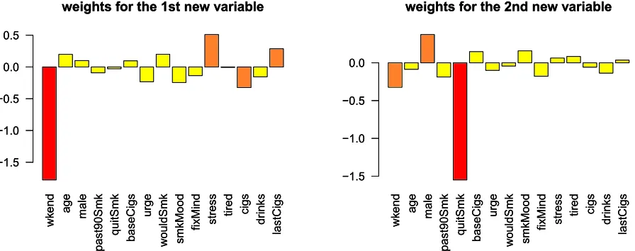
Figure 2.4 Weights of the original variables in the first two components of the estimated feature map. . . 31

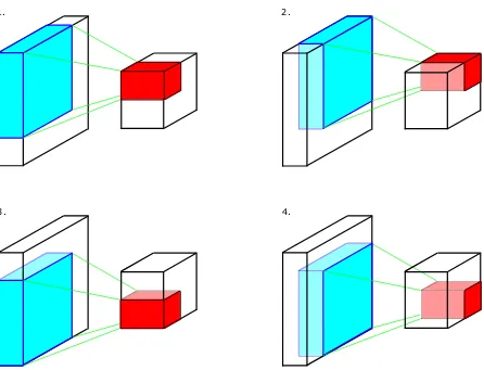
Figure 2.5 The convolution operation in ConvNets. In this example, each input feature map is 4_×4; each output feature map is 2_×2; the kernel’s first two dimensions are 3_×3; the stride size is 1; there is no padding; the convolution takes 4 steps. . . 35

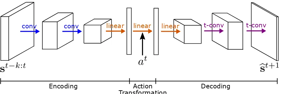
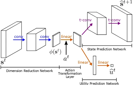
Figure 2.6 The architecture of Action-Conditional Video Prediction Network (Oh et al., 2015). The blue, orange, and purple arrows indicate convo-lution, linear transformation, and transposed convolution respectively. 37 Figure 2.7 The architecture of Convolutional Alternating Deep Neural Network. 40 Figure 2.8 The simplified architecture of Convolutional Alternating Deep Neural Network. . . 42

Figure 2.9 Screenshots from the games used as testbeds. From left to right, top to bottom: Catcher, Pong, Pixelcopter, FlappyBird. . . 43

Figure 3.1 Overview of the ordinal regression neural network for text input.h represents hidden state (details explained in the following subsec-tions). . . 53

Figure 3.2 The Skip-gram model architecture. . . 55

Figure 3.3 A basic multi-layered RNN. . . 56

Figure 3.4 A Gated-feedback RNN. . . 57

Figure 3.5 Ordinal regression layer. . . 59

Figure 3.6 Emoji map produced by applying t-SNE to the emojis’ vectors learned from escort ads using skip-gram model. For visual clarity, only the emojis that appeared most frequently in the escort ads we scraped are shown out of the total 968 emojis that appeared. See Appendix C.5 for maps of other emojis. . . 67

(12)

Figure C.2 Emoji map produced by applying t-SNE to the emojis’ vectors learned from escort ads using skip-gram model. For visual clarity, only the emojis with frequency ranking 401–600 are shown; outliers were re-moved for better zoom. . . 107 Figure C.3 Emoji map produced by applying t-SNE to the emojis’ vectors learned

from escort ads using skip-gram model. For visual clarity, only the emojis with frequency ranking 601–800 are shown; outliers were re-moved for better zoom. . . 108 Figure C.4 Emoji map produced by applying t-SNE to the emojis’ vectors learned

(13)

CHAPTER 1 THEORETICAL FRAMEWORK OF

SUFFICIENT MARKOV DECISION

PROCESSES

1.1 Introduction

Sequential decision problems arise in a wide range of application domains including

au-tonomous vehicles (Bagnell and Schneider, 2001), finance (Bäuerle and Rieder, 2011),

logistics (Zhang and Dietterich, 1995), robotics (Kober et al., 2013), power grids (Riedmiller

et al., 2000), and healthcare (Chakraborty and Moodie, 2013). Markov decision processes

(MDPs) (Bellman, 1957; Puterman, 2014) are the primary mathematical model for

(14)

Tsitsiklis, 1996; Sutton and Barto, 1998; Bather, 2000; Si, 2004; Powell, 2007; Wiering and

Van Otterlo, 2012). This class of models is quite general as almost any decision process can

be made into an MDP by concatenating data over multiple decision points (see Section 1.2

for a precise statement); however, coercing a decision process into the MDP framework in

this way can lead to high-dimensional system state information that is difficult to model

effectively. One common approach to construct a low-dimensional decision process from

a high-dimensional MDP is to create a finite discretization of the space of possible system

states and to treat the resultant process as a finite MDP (Gordon, 1995; Murao and

Kita-mura, 1997; Sutton and Barto, 1998; Kamio et al., 2004; Whiteson et al., 2007). However,

such discretization can result in a significant loss of information and can be difficult to

apply when the system state information is continuous and high-dimensional. Another

common approach to dimension reduction is to construct a low-dimensional summary

of the underlying system states, e.g., by applying principal components analysis (Jolliffe,

1986), multidimensional scaling (Borg and Groenen, 1997), or by constructing a local linear

embedding (Roweis and Saul, 2000). These approaches can identify a low-dimensional

representation of the system state but, as we shall demonstrate, they need not retain salient

features for making good decisions.

The preceding methods seek to construct a low-dimensional representation of a

high-dimensional MDP with the goal of using the low-high-dimensional representation to estimate

an optimal decision strategy, i.e., one that leads to maximal mean utility when applied to

the original process; however, they offer no guarantee that the resulting process is an MDP

or that a decision strategy estimated using data from the low-dimensional process will

perform well when applied to the original process. We derive sufficient conditions under

which a low-dimensional representation is an MDP, and that an optimal decision strategy

(15)

hypothesis test for this sufficient condition based on the Brownian distance covariance

(Székely et al., 2007; Székely and Rizzo, 2009) and use this test as the basis for evaluating a

dimension reduction function.

In Section 1.2, we review the MDP model for sequential decision making and define

an optimal decision strategy. In Section 1.3, we derive conditions under which a

low-dimensional representation of an MDP is sufficient for estimating an optimal decision

strategy for the original process. In Section 1.4, we discuss the challenges for designing

a dimension reduction function that can produce the aforementioned low-dimensional

representation, which will motivate our new deep learning algorithm described in Chapter

2.

1.2 Setup and Notation

We assume that the observed data are S1

i,A

1

i,U

1

i ,S

2

i, . . . ,A T i ,U

T i ,S

T+1

i n

i=1which comprise

n independent and identically distributed copies of the trajectory(S1_,_A1_,_U1_,_S2_{, . . . ,}_AT_, UT_,_ST+1₎ _where:_T _∈

Ndenotes the observation time; St ∈ Rpt _{denotes a summary of}

information collected up to time t =1, . . . ,T;At _{∈ A} ₌_{_{1, . . . ,}_K_}_{denotes the decision} made at timet =1, . . . ,T; andUt ₌_Ut₍_St_,_At_,_St+1₎_{is a real-valued deterministic function}

of(St,At_,_St+1₎_{that quantifies the momentary “goodness”}1 _{of being in state}_St_{, making} decision At_{, and subsequently transitioning to state}_St+1_{. We assume throughout that}

sup_t_|Ut_{| ≤}_M _{with probability one for some fixed constant}_M_{. In applications like mobile} health, the observed data might be collected in a pilot study with a preset time horizon

(16)

when applied over an indefinite time horizon (Ertefaie, 2014; Liao et al., 2015; Luckett et al.,

2016). Thus, we view the observed trajectory(S1_,_A1_,U1_,_S2_{, . . . ,}_AT_,UT_,_ST+1₎_{as a truncation}

of the infinite process(S1_,_A1_,_U1_,_S2_{, . . .}₎_{. Furthermore, we assume (A0) that this infinite}

process is Markov and homogeneous in that it satisfies

P

St+1∈ Gt+1

At,St, . . . ,A1,S1

=P

St+1∈ Gt+1

At,St

, (1.1)

for all (measurable) subsets_Gt+1 _⊆ _dom_St+1 _and _t _∈

Nand that the probability mea-sure in (1.1) does not depend ont. For any process(S1_,_A1_,U1_,_S2_{, . . .}₎_{one can define}

e St ₌

(St_,Ut−1_,_At−1_{, . . . ,}_St−mt)_{, where}_m

tis chosen so that process eS1,A1,U1,eS2, . . .

satisfies (A0);

to see this, note that the result holds trivially formt =t−1. Furthermore, by augmenting the state with a variable for time, i.e., defining the new state at timet to be(eSt,t), one can ensure that the probability measure in (A0) does not depend on t. In practice,mt is typically chosen to be a constant, as letting the dimension of the state grow with time

makes extrapolation beyond the observed time horizon,T, difficult. Thus, hereafter we assume that the domain of the state is constant over time, i.e., domSt ₌_{S ⊆}

Rpfor allt ∈N. Furthermore, we assume that the utility is homogeneous in time, i.e.,Ut ₌_U₍_St_,_At_,_St+1₎

for allt ∈N.

A decision strategy,π:S → A, is a map from states to decisions so that, underπ, a

deci-sion maker presented withSt =st at timet will select decisionπ(st). We define an optimal decision strategy using the language of potential outcomes (Rubin, 1978). We use an overline

to denote history so thatat = (a1_{, . . . ,}_at₎_and_st

= (s1_{, . . . ,}_st₎_{. The set of potential outcomes}

isO∗₌

S∗t₍_at−1₎

t≥1whereS

∗t₍_at−1₎

is the potential state underat−1and we have defined

S∗1₍_a0_{) =}

S1_{. Thus, the potential utility at time}_t _under_at

isUS∗t₍_at−1₎

(17)

potential state under a decision strategy,π, is

S∗t(π) =X

at−1

S∗t(at−1) t−1

Y

v=1

1_π_{_S∗v₍_av−1₎_}₌_av,

and the potential utility underπis

U∗t(π) =US∗t(π),πS∗t(π) ,S∗(t+1)(π).

Define the discounted mean utility under a decision strategy,π, as

V(π) =E ¨

X

t≥1

γt−1_U∗t_(π) «

,

whereγ_∈(0, 1)is a discount factor that balances the trade-off between immediate and

long-term utility. Given a class of decision strategies,Π, an optimal decision strategy,πopt_∈_Π_,

satisfiesV(πopt₎_≥_V_(π)_{for all}_π_∈_Π_.

Define the action selection probability during data generation as

µt₍_at_;_st

,at−1) =PAt =atS t

=st,At−1=at−1.

To characterizeπoptin terms of the data-generating model, we make the following

assump-tions for allt ∈N:

(C1) consistency,St ₌_S∗t₍_At−1₎_;

(18)

These assumptions are standard in data-driven decision making (Robins, 2004; Schulte

et al., 2014). Assumptions (C2) and (C3) hold by design in a randomized trial (Liao et al.,

2015; Klasnja et al., 2015) but are not verifiable in the data for observational studies. Under

these assumptions, the joint distribution of_{S∗t_(π)}T

t=1is non-parametrically identifiable

under the data-generating model for any decision strategyπand time horizonT. In our application, these assumptions will enable us to construct low-dimensional features of

the state that retain all relevant information for estimatingπopt_{without having to solve the}

original MDP as an intermediate step.

1.3 Theoretical Results

If the statesSt are high-dimensional it can be difficult to construct a high-quality estimator

of the optimal decision strategy; furthermore, in applications like mobile health, storage

and computational resources on the mobile device are limited, making it desirable to store

only as much information as is needed to inform decision making. For any mapφ:_{S →}_Rq

defineSt

φ=φ(St). We say thatφinduces a sufficient MDP forπoptif(A t

,St_φ+1,Ut)contains all relevant information in(At,St+1,Ut)aboutπopt_{. Given a policy}_π

φ: domSt_φ→ A define

the potential utility underπ_φas

U_φ∗t(π_φ) =X

at

U S∗t at−1,at,S∗(t+1) at t Y

v=1

1_π φ

¦

S∗_φv(av−1)©

=av.

The following definition formalizes the notion of inducing a sufficient MDP.

Definition 1.3.1. LetΠ _{⊆ A}S _{denote a class of decision strategies defined on}_S _and

Πφ⊆ ASφ a class of decision strategies defined onSφ=domSφt ⊆Rq. We say that the pair

(19)

t ∈N:

(S1) the process(At,St_φ+1,Ut)is Markov and homogeneous, i.e.,

PS_φt+1_{∈ G}_φt+1S t φ,A

t

=PS_φt+1_{∈ G}_φt+1St_φ,At

for any (measurable) subset_Gt+1

φ ⊆Rq and this probability does not depend ont;

(S2) there existsπopt_∈_{arg max}

π∈ΠV(π)which can be written asπopt=π

opt

φ ◦φ, where

πopt

φ ∈arg max_π_φ_∈_Π_φE ¨

X

t≥1

γt−1_U∗t φ (πφ)

« .

Thus, given the observed data,¦ST_i+1,AT_i ,UT_i ©n

i=1and class of decision strategies,Π, if one

can find a pair(φ,Π_φ)which induces a sufficient MDP forπopt_within_Π_{, then it suffices to}

store only the reduced process¦ST_φ+_,_i1,AT_i ,UT_i ©n

i=1. Furthermore, existing reinforcement

learning algorithms (see Appendix A.1 and e.g., Sutton and Barto, 1998; Szepesvári, 2010) can

be applied to this reduced process to construct an estimator ofπopt_φ and henceπopt₌_πopt

φ ◦φ.

If the dimension ofSt_φis substantially smaller than that ofSt, then using the reduced process

can lead to smaller estimation error as well as reduced storage and computational costs.

In some applications, it may also be desirable to haveφbe a sparse function ofSt _{in the}

sense that it only depends on a subset of the components ofSt_{. For example, in the context}

of mobile health, one may construct the state,St_{, by concatenating measurements taken at}

time pointst,t−1, . . . ,t−m, where the look-back period,m, is chosen conservatively based on clinical judgement to ensure that the process is Markov; however, a data-driven sparse

(20)

of clinical value. The remainder of this section will focus on developing verifiable conditions

for checking that(φ,Π_φ)induces a sufficient MDP. These conditions are used to build a

data-driven, low-dimensional, and potentially sparse sufficient MDP.

DefineYt+1=Ut_,₍_St+1₎ü ü_{for all}_t _∈

N. The following result provides a conditional independence criterion that ensures a given feature map induces a sufficient MDP; this

criterion can be seen as an MDP analog of nonlinear sufficient dimension reduction in

regression (Cook, 2007; Li et al., 2011). A proof is provided in Appendix A.2.

Theorem 1.3.2. Let(S1,A1_,_U1_,_S2_{, . . .}₎_{be an MDP that satisfies (A0) and (C1)-(C3). Suppose}

that there existsφ:_{S →}_Rq _{such that}

Yt+1_⊥_⊥StSt_φ,At, (1.2)

then,(φ,Π_φ,msbl)induces a sufficient MDP for πopt _within_Π

msbl, whereΠmsbl is the set of

measurable maps fromS intoA andΠ_φ,msblis the set of measurable maps fromRq intoA.

The preceding result could be used to construct an estimator for φ so that(φ,Π_φ,msbl)

induces a sufficient MDP forπopt_within_Π

msbl as follows. LetΦdenote a potential class

of vector-valued functions on_S. Letp_bn(φ)denote a p-value for a test of the conditional independence criterion (1.2) based on the mappingφ, e.g., one might construct this

p-value using conditional Brownian distance correlation (Wang et al., 2015) or kernel-based

tests of conditional independence (Fukumizu et al., 2007). Then, one could selectφÒ_n to

be the transformation of lowest dimension among those within the setφ_∈Φ:p_bn(φ)< τ , whereτis a fixed significance level, e.g.,τ =0.10. However, such an approach can be

computationally burdensome especially if the classΦis large. Instead, we will develop a

procedure based on a series of unconditional tests that is computationally simpler and

(21)

first describe how the conditional independence criterion in the above theorem can be

applied recursively to potentially produce a sufficient MDP of lower dimension.

The conditionYt+1_⊥_⊥_St

St_φ,At is overly stringent in that it requiresSt_φto capture all the information aboutYt+1contained withinSt _{regardless of whether or not that information} is useful for decision making. However, given a sufficient MDP(S1

φ,A1,U1,S2φ, . . .), one can apply the above theorem to this MDP to obtain further dimension reduction; this process

can be iterated until no further dimension reduction is possible. For any mapφ:S →Rq,

defineY_φt =¦Ut_,_St+1

φ ü©ü

. The following result is proved in Appendix A.3.

Corollary 1.3.3. Let(S1_,_A1_,_U1_,_S2_{, . . .}₎_{be an MDP that satisfies (A0) and (C1)-(C3). Assume}

that there existsφ0:_{S →}_Rq0_{such that}_(φ0_,_Π

φ0,msrbl)induces a sufficient MDP forπ

opt_within

Πmsrbl. Suppose that there existsφ1:Rq0→Rq1such that for all t ∈N

Yt_φ+1 0 ⊥⊥S

t φ0

St_φ

1◦φ0,A t

, (1.3)

then(φ1◦φ0,Π_φ₁_◦_φ₀_,msrbl)induces a sufficient MDP forπopt_within_Π

msrbl. Furthermore, for

k≥2, denotingφk◦φk−1◦ · · · ◦φ0byφk, if there existsφk:Rqk−1→Rqk such that

Yt_φ+1

k−1 ⊥⊥ S_φt

k−1 St

φk,A

t ,

then(φ_k,Π_φ

k,msrbl)induces a sufficient MDP forπ

opt_within_Π msrbl.

We now state a simple condition involving the residuals of a multivariate regression that

can be used to test the conditional independence required in each step of the preceding

corollary. In our implementation we use residuals from a variant of deep neural networks

(22)

Lemma 1.3.4. Let(S1,A1_,U1_,_S2_{, . . .}₎_{be an MDP that satisfies (A0) and (C1)-(C3). Suppose}

that there existsφ:_{S →}_Rq _{such that at least one of the following conditions holds:}

(i) ¦Yt+1₋_EYt+1St_φ,At ©

⊥⊥St At,

(ii) ¦St₋ E

St

St_φ ©

⊥⊥Yt+1,St φ

At,

thenYt+1_⊥_⊥St St_φ,At.

The preceding result can be used to verify the conditional independence condition required

by Theorem (1.3.2) and Corollary (1.3.3) using unconditional tests of independence within

levels ofAt_{; in our simulation experiments, we used Brownian distance covariance for} continuous states (Székely et al., 2007; Székely and Rizzo, 2009) and a likelihood ratio test

for discrete states, though other choices are possible (Gretton et al., 2005a,b). Application of

these tests requires modification to account for dependence over time within each subject.

One simple approach, the one we follow here, is to compute a separate test at each time

point and then to pool the resultant p-values using a pooling procedure that allows for

general dependence. For example, letGt ₌_g₍_St_,_At_,_St+1₎_∈

Rd1 andHt =h(_St)∈

Rd2 be known features of(St_,_At_,_St+1₎_and_St_{. Let}

Pndenote the empirical measure. To testGt ⊥⊥Ht using the Brownian distance covariance, we compute the test statistic

b

Tt_n = ||Pnexp

i ςü_Gt+%ü_H

t −Pnexp iςüGt

Pnexp i%üGt

||2_ω

=

Z Pnexp

i ςü_Gt+%ü_H

t −Pnexp(iςüGt)Pnexp i%üHt 2

Γ 1+d1

2

Γ 1+d2

2

||ς||d1+1||%||d2+1_π(d1+d2+2)/2 d%dς,

and subsequently compute thep-value, sayp_bt

n, using the null distribution ofTb_nas estimated by permutation (see Appendix A.7 for the algorithm, and Székely et al., 2007; Székely and

Rizzo, 2009, for more details). For eachu=1, . . . ,T, letp_b(u)

(23)

b p1

n, . . . ,pb T

n and define the pooledp-value

b

p_nu_,pooled=Tpb (u) n u .

For eachu=1, . . . ,T it can be shown thatp_bu

n,pooledis validp-value (Rüger, 1978), e.g.,u =1

corresponds to the common Bonferroni correction. In our simulation experiments, we set

u =bT/20+1_cacross all settings (see Appendix A.8 for more details).

1.3.1 Variable Screening

The preceding results provide a pathway for constructing sufficient MDPs. However, while

the criteria given in Theorem 1.3.2 and Lemma 1.3.4 can be used to identify low-dimensional

structure in the state, they cannot be used to eliminate certain simple types of noise

vari-ables. For example, letBt _t

≥1denote a homogeneous Markov process that is

indepen-dent of (S1_,_A1_,U1_,_S2_{. . .}₎_{, and consider the augmented process}

e

S1_,_A1_,U1_,

e S2_{, . . .}

, where

e

St =(St)ü_,(_Bt)ü ü_{. Clearly, the optimal policy for the augmented process does not depend}

onBt _t

≥1, yet,Y

t+1_{need not be conditionally independent of}

e

St givenSt. To remove

vari-ables of this type, we develop a simple screening procedure that can be applied prior to

constructing nonlinear features as described in the next section.

The proposed screening procedure is based on the following result which is proved in

Appendix A.5.

Theorem 1.3.5. Let(S1_,_A1_,_U1_,_S2_{, . . .}₎_{be an MDP that satisfies (A0) and (C1)-(C3). Suppose}

that there existsφ:S →Rq such that

(24)

then,(φ,Π_φ,msbl)induces a sufficient MDP for πopt _within_Π

msbl, whereΠmsbl is the set of

measurable maps fromS intoA andΠ_φ,msblis the set of measurable maps fromRq intoA.

This result can be viewed as a stronger version of Theorem 1.3.2 in that the required

condi-tional independence condition is weaker; indeed, in the example stated above, it can be

seen thatφ(eSt) =St satisfies (1.4). However, becauseφappears in bothYt_φ+1andS_φt, con-structing nonlinear features using this criterion is more challenging as the residual-based

conditions stated in Lemma 1.3.4 can no longer be applied. Nevertheless, this criterion

turns out to be ideally suited to screening procedures wherein the functionsφ:_Rp_→ Rq are of the formφ(st₎

j =sktj for j =1, . . . ,q, where

k1, . . . ,kq is a subset of

1, . . . ,p .

For any subset J ⊆1, . . . ,p , defineSt J =

¦ St

j ©

j∈J andY t J =

Ut_,₍_St

J)ü . Let J1 denote

the smallest set of indices such thatUt _{depends on}_St _and_St+1_{only through}_St

J1andS t+1

J1

conditioned on At_{. For} _k _≥ _{2, define} _J k =

¦

1_≤j≤p :St j 6⊥⊥Y

t Jk−1

At

©

. LetK denote the smallest value for which JK−1= JK, such aK must exist as Jk−1⊆ Jk for allk, and define

φscreen(St) = St_J

K. The following result (see Appendix A.6 for a proof ) shows thatφscreen

induces a sufficient MDP; furthermore, Corollary 1.3.3 shows that such screening can be

applied before nonlinear feature construction without destroying sufficiency.

Theorem 1.3.6. Let(S1_,_A1_,U1_,_S2_{, . . .}₎_{be an MDP that satisfies (A0) and (C1)-(C3), and let}

J1, . . . ,JK,φscreen be as defined above. Assume that for any two non-empty subsets, J,J0⊆

1, . . . ,p , ifSt J 6⊥⊥Y

t+1

J0

At then there exists j ∈J such that S_jt 6⊥⊥Yt_J+₀1

At. Then,

Yt_φ+1 screen⊥⊥S

t St_φ

screen,A t_.

The condition that joint dependence implies marginal dependence (or equivalently, marginal

independence implies joint independence) ensures that screening one variable at a time

(25)

by considering sets of multiple variables at a time though at the expense of additional

com-putational burden. Algorithm 1 gives a schematic for estimatingφscreenusing the Brownian

distance covariance to test for dependence. The inner for-loop (lines 4-7) of the algorithm

can be executed in parallel and thereby scaled to large domains.

Algorithm 1Screening with Brownian Distance Covariance

Input: p-value thresholdτ; max number of iterationsNmax; data

¦

ST_i+1,AT_i ,UT_i ©n

i=1; set of

all indicesD ={1, 2, . . . ,p=dim(St_)}_.

1: Set J0=;, andYt_J0+1={Ut}

2: fork=1, . . . ,Nmaxdo

3: Set Jk=Jk−1

4: for each j ∈D\Jk−1do

5: Perform dCov test onSt j andY

t+1

Jk−1 within levels ofA t

6: ifp-value_≤τthen

7: SetJk =Jk∪ {j}

8: if Jk =Jk−1then

9: SetK =k, stop. Output: JK

1.4 Discussion

Theorem 1.3.2, Corollary 1.3.3, and Theorem 1.3.5 provide general conditions that a

di-mension reduction functionφshould meet to retain all relevant information regardless

of the implementations of hypothesis tests for those conditions or howφÒis constructed.

We presented a Brownian distance covariance based test for checking the conditions in

Section 1.3, and we will present our deep neural network algorithm for constructingφÒin

(26)

should have.

Condition 1.2 suggests that in the context of MDPs, a sufficient dimension reduction

needs to retain the information inSt _{relevant to}_Yt+1_{. Thus, the goal is very different from}

the goal of common dimension reduction techniques, which is usually to retain information

about the original input,St _{in this case. Common techniques like principal components}

analysis (PCA) (Jolliffe, 1986) and autoencoder (Bengio, 2009; Vincent et al., 2010) can

discard redundant information fromSt, e.g., whenSt has some highly correlated variables,

but they are not designed to discard noisy information irrelevant toYt+1. Imagine thatSthas a few independent variables that don’t affectYt+1_{at all. PCA and autoencoder will keep the}

information of these variables, because they contribute to the variance ofSt _{and cannot be}

reconstructed from the other variables inSt_{. In general, any dimension reduction technique}

that doesn’t evaluate the relationship betweenSt _and_Yt+1_{is unlikely to be efficient.}

Therefore, it seems the most reasonable approach to perform supervised learning and

build a model that predictsYt+1fromSt, and then obtainφÒfrom the predictive model. For example, if the model is a deep neural network (DNN) (LeCun et al., 2015) whose input isSt

and output isEb[Yt+1|St], thenφ(ÒSt)could be the the output from an intermediate/hidden layer with lower dimension thanSt_.

However, another challenge arises: The relationship betweenSt _and_Yt+1_{often depends}

onAt_{, and the relevant information for}_Yt+1_in_St _{could be different for different levels of} At_{. So a good predictive model will predict}

b

E[Yt+1_|St_,_At_]_{differently for each level of}_At_{. In} the mean time, the computation ofφ(ÒSt)cannot depend onAt.φ(ÒSt)should contain the union of relevant information forYt+1for all possible levels ofAt_{, because eventually we} wish to apply the estimated optimal policy to new data, and useat₌_argmax

aQÒ∗(φ(Òst),a) for action selection. Naturally, we needφ(ÒSt)before knowingAt.

(27)

the predictive model should capture the relationship betweenSt andYt+1unique toAt by making different predictions accordingly;φ(ÒSt)should be the same and contain the

relevant information forYt+1_{no matter what}_At _{turns out to be. Going back to the DNN} example where we letφ(ÒSt)be the output from a hidden layer, if we train a different network

for each level ofAt _{or include}_At _{in the input, the computation of} Ò

φ(St₎_{will depend on}_At_;

if we completely ignoreAt_{, then the network will try to learn the potentially conflicting} At-specific relationships betweenSt andYt+1all at once, making the network intrinsically unstable. This motivates us to design a new deep learning algorithm, Alternating Deep

Neural Networks (see Chapter 2), that can learnAt_{-specific relationships separately while} constructing anAt_-indifferent

Ò

(28)

CHAPTER 2 CONSTRUCTING SUFFICIENT MARKOV

DECISION PROCESSES WITH

ALTERNATING DEEP NEURAL

NETWORKS

2.1 Introduction

Deep neural networks (DNNs) have recently become a focal point in machine learning

research because of their ability to identify complex and nonlinear structure in

high-dimensional data (see Anthony and Bartlett, 2009; LeCun et al., 2015; Goodfellow et al.,

(29)

construction. To address the challenges mentioned in Section 1.4, we propose a novel

variation of DNNs. Before explaining the details of our algorithm, we will briefly introduce

DNNs.

DNNs are essentially artificial neural networks (ANNs) with many hidden layers and

various improvements (see Goodfellow et al., 2016, and references therein). ANNs are

inspired by biological neural networks. An ANN model is usually composed of an input

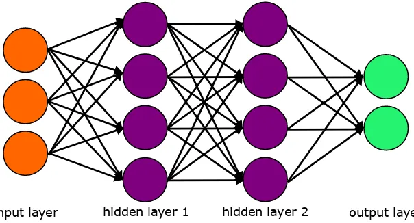
layer, one or several hidden layers, and an output layer (Figure 2.1). Data are propagated

forward through the network via linear transformations between layers followed by possibly

non-linear activation functions within each layer to obtain the output. More precisely, for

thel-th layer, letOl−1_∈

Rp×1be the input,wl ∈Rq×pbe the weight matrix,bl ∈Rq×1be the intercept vector1_,_ξl _{be the element-wise activation function which is typically sigmoid or}

rectified linear unit, andOl _∈

Rq×1be the output, then

Ol =ξl(wl ·Ol−1+bl).

LetXi =O1_i be thei-th initial input,Ybi =OL_i be thei-th final output,θ be the set of all parameters. The network is trained to minimize a cost function, typically the root mean

squared error of predictions:

C(θ) = v u t1

n n X

i=1

kYi−bYik22.

The gradient of the cost function is propagated backwards through the network to update

all the parameters using Stochastic Gradient Descent or its variations.

DNNs are theoretically capable of efficiently yielding more flexible function

(30)

input layer hidden layer 1 hidden layer 2 output layer

Figure 2.1 A basic artificial neural network with 2 hidden layers.

tion and better performance than “shallow” ANNs (Bengio, 2009). However, because the

gradients of early layers are products of the gradients of the subsequent layers by the chain

rule, they tend to vanish or explode when the number of layers is increased naively, making

DNNs difficult to train (Bengio, 2009). Researchers have developed a variety of methods to

enable the training and enhance the performance of DNNs, such as layer by layer

pretrain-ing (Hinton and Salakhutdinov, 2006; Vincent et al., 2010), uspretrain-ing Convolutional Network

for image data (Nielsen, 2015), performingL1 orL2regularizations, adding drop-out to

hidden layers (Srivastava et al., 2014) and so on. The advancement of computer hardware,

especially Graphical Processing Units, also played a big role in the rise of popularity of

DNNs (LeCun et al., 2015). On top of some of the aforementioned enhancements, we add

a new structure and training procedure to DNNs to construct the dimension reduction

functionφÒ, so that we can solve the dilemma thatφÒshould not depend onAt while the predictionEb[Yt+1|St,At]should.

In Section 2.2, we describe our proposed algorithm that is designed to produce a

low-dimensional representation that satisfies the proposed sufficient condition from Theorem

(31)

simulation experiments. In Section 2.4, we illustrate the proposed method using data from a

study of a mobile health intervention targeting smoking and heavy episodic drinking among

college students (Witkiewitz et al., 2014). In Section 2.5, we discuss some shortcomings of the

main algorithm and several directions it can be extended. In Section 2.6, we complete one

such extension that allows our algorithm to handle states in the form of multi-dimensional

arrays such as image frames in video games.

2.2 Method

We inherit the notations on Markov decision processes (MDPs) from Chapter 1. Section 2.1

describes deep neural networks (DNNs) on a high level with notations commonly used in

the literature; in this section we will re-describe DNNs with slightly different notations more

suitable in our feature construction/dimension reduction framework. For simplicity, we assume that_S =_Rp_{. We consider summary functions}_φ_:

Rp→Rq that are representable as DNNs. Here, we present a novel neural network architecture for estimating sufficient

MDPs.

We use criterion (i) in Lemma 1.3.4 to construct a data-driven summary functionφ,

therefore we also require a model for the regression ofYt+1 onSt

φ andAt; we also use a DNN for this predictive model. Thus, the model can be visualized as two DNNs: one

that composes the feature mapφand another that models the regression ofYt+1onSt_φ andAt_{. A schematic for this model is displayed in Figure 2.2. Let}_Φ_:

R→[0, 1]denote a continuous and monotone increasing function and writeΦ◦_{to denote the vector-valued}

function obtained by elementwise application ofΦ, i.e.,Φ◦

j(v) =Φ(vj)wherev ∈R d_{. The}

(32)

thatr1=p. The first layer of the feature map network is

L1(s;Σ₁,η1) =Φ◦ Σ₁s+η1,

whereΣ1∈Rr2×r1andη1∈Rr2. Recursively, fork=2, . . . ,M1, define

Lk(s;Σk,ηk, . . . ,Σ1,η1) =Φ◦

ΣkLk−1 s;Σk−1,ηk−1, . . . ,Σ1,η1

+ηk ,

whereΣk ∈Rrk×rk−1 andηk∈Rk. Letθ1= ΣM1,ηM1, . . . ,Σ1,η1

, then the feature map under

θ1is

φ(s;θ1) =_L_M1(s;θ1) =_L_M1 s;Σ_M1,η_M1, . . . ,Σ₁,η1.

Thus, the dimension of the feature map isrM1. The neural network for the regression of Yt+1_on_St

φandAt is as follows. LetrM1+1, . . . ,rM1+M2 ∈Nbe such thatrM1+M2=p+1. For each a ∈ A define

LM1+1,a(s;θ1,ΣM1+1,a,ηM1+1,a) =Φ◦

ΣM1+1,aφ(s;θ1) +ηM1,a ,

whereΣ_M1₊_1,_a _∈_RrM1+1×rM1 andη

M1,a∈RrM1+1. Recursively, fork =2, . . . ,M2and eacha ∈ A

define

LM1+k,a s;θ1,ΣM1+k,a,ηM1+k,a, . . . ,ΣM1+1,a,ηM1+1,a

=Φ◦

ΣM1+k,aLM1+k−1,a s;θ1,ΣM1+k−1,a,ηM1+k−1,a, . . . ,ΣM1+1,a,ηM1+1,a

+ηM1+k,a ,

whereΣM1+k,a ∈R

rM₁+k×rM₁+k−1 _andη

M1+k∈R

rM₁+k_{. For each}_a _{∈ A}_{, define}

θ2,a = ΣM1+M2,a,ηM1+M2,a, . . . ,ΣM1+1,a,ηM1+1,a

(33)

and writeθ2=θ2,_a _a

∈A. The postulated model forE

Yt+1

St_φ=s_φt,At =at

under

parame-ters(θ1,θ2)is_L_M1₊_M1(s;θ1,θ2,_at).

We use penalized least squares to construct an estimator of(θ1,θ2). LetPndenote the

empirical measure and define

C_nλ(θ1,θ2) =_P_n T X

t=1

||LM1+M2(St;θ1,θ2,At)−Yt+1||2+λ

r1 X

j=1

v u t r2 X `=1 Σ2

1,`,j, (2.1)

and subsequently θb_1,λ_n,θb_2,λ_n

=arg min_θ₁_,_θ₂C_nλ(θ1,θ2), whereλ >0 is a tuning parameter.

The termqP_`=r2₁Σ2

1,`,j is a group-lasso penalty (Yuan and Lin, 2006) on the`th column

ofΣ1; if the`th column ofΣ1 shrunk to zero thenSt_φdoes not depend on the`th

com-ponent ofSt. Computation of θb_1,λ_n,θb_2,λ_n

also requires choosing values forλ,M1,M2, and

r2, . . . ,rM1−1,rM1+1, . . . ,rM1+M2−1, (recall thatr1=p,rM1+M2 =p+1, andrM1is the dimension of the feature map and is therefore considered separately). Tuning each of these parameters

individually can be computationally burdensome, especially whenM1+M2is large. In

our implementation, we assumed r2 =r3 =· · ·= rM1−1 = rM1+1 =· · ·= rM1+M2−1= K1and

M1=M2=K2; then, for each fixed value ofrM1 we selected(K1,K2,λ)to minimize cross-validated cost. Algorithm 2 shows the process for fitting this model; the algorithm uses

subsampling to improve stability of the underlying sub-gradient descent updates (this is

also known as taking minibatches, see Lab, 2014; Goodfellow et al., 2016, and references

therein).

To select the dimension of the feature map we choose the lowest dimension for which

the Brownian distance covariance test of dependence betweenYt+1_−L

M1+M2(St;θ1,b _n,θ2,b _At_,_n)

andSt _{fails to reject at a pre-specified error level}_τ_∈₍_{0, 1}₎_{. Let} Ò

φ1

(34)

Algorithm 2Alternating Deep Neural Networks

Input: Tuning parameters K1,K2 ∈ N, λ ≥ 0; feature map dimension r1; data

¦

i=1; batch size proportionν∈(0, 1); gradient-descent step-size{αb}b≥1;

error toleranceε >0; max number of iterations Nmax; and initial parameter values

b

θ(1)

1,n,θb(

1)

2,n.

1: SetDa =

(i,t): At

i =a andna =#Da for eacha ∈ A andt =1, . . . ,T

2: forb =1, . . . ,Nmaxdo

3: for eacha ∈ A do

4: Draw a random batchBa of sizebνnacwithout replacement fromDa

5: Compute a sub-gradient of the cost on batchBa

Λ(b) a =∇



 1

bνnac X

(i,t)∈Ba

L_M

1+M2

S_it;θb_1,(b_n),θb_2,(b_a)_,_n −Yt_i+1 2 +λ r1 X

j=1

v u t r2 X `=1 Σ2 1,`,j





6: Compute a sub-gradient descent update

b

θ(b+1)

1,n

b

θ(b+1)

2,a,n

=

b

θ(b)

1,n

b

θ(b)

2,a,n

+αbΛ(_ab)

7: Setθb( b+1)

2,a0,n=θb( b)

2,a0,nfor alla06=a

8: If maxa

C_nλθb( b+1)

1,n ,θb( b+1)

2,a,n −Cnλ

b

θ(b)

1,n,θb( b)

2,a,n ≤ε

stop.

Output: θ1,b _n,θ2,b _n

= θb( b+1)

1,n ,θb( b+1)

(35)

Figure 2.2 Schematic for alternating deep neural network (ADNN) model. The term “alternating” refers to the estimation algorithm which cycles over the networks for each treatmenta∈ A.

maps_{7→ L}_M1(s;θ1)b . Define

b

R_n1=¦j ∈ {1, . . .r1}: Σb

2

to be the elements ofSt_{that dictate}_St

Ò

φ1

n

; writeSt

b

R1

nas shorthand for

¦ St

j ©

j∈Rbn1

. One may wish to

iterate the foregoing estimation procedure as described in Corollary 1.3.3. However, because

the components ofSt

Ò

φ1

n

are each a potentially nonlinear combination of the elements ofSt

b

R1

n,

therefore a sparse feature map defined on the domain ofSt

Ò

φ1

n

may not be any more sparse in

terms of the original features. Thus, when iterating the feature map construction algorithm,

we recommend using the reduced process¦ST+1

b

Rn1,i,A

T i,U

T i

©n

i=1and the input; because the

sigma-algebra generated bySt

b

R1

n contains the sigma-algebra generated byS

t

Ò

φ1

n, this does not

incur any loss in generality. The above procedure can be iterated until no further dimension

(36)

2.3 Simulation Experiments

We evaluate the finite sample performance of the proposed method (pre-screening with

Brownian distance covariance +iterative alternating deep neural networks, which we will simply refer to as ADNN in this section) using a series of simulation experiments. To

form a basis for comparison, we consider two alternative feature construction methods:

(PCA) principal components analysis, so that the estimated feature map φPCA(Ò s) is the

projection ofsonto the firstkprincipal components ofT−1PT

t=1Pn{S

t₋

PnSt} {St−PnSt}ü; and (tNN) a traditional sparse neural network, which can be seen as a special case of our

proposed alternating deep neural network estimator where there is only 1 action. In our

implementation of PCA, we choose the number of principal components,k, corresponding to 90% of variance explained. We do not compare with sparse PCA for variable selection,

because based on preliminary runs, the principal components that explain 50% of variance

already use all the variables in our generative model. In our implementation of tNN, we

build a separate tNN for eacha ∈ A, where(λ,K1,K2,r1)are tuned using cross-validation,

and take the union of selected variables and constructed features. Note that there is no other

obvious way to join the constructed features from tNN but to simply concatenate them,

which will lead to inefficient dimension reduction especially when_{|A |}is large, whereas we

will see that ADNN provides a much more efficient way to aggregate the useful information

across actions.

We evaluate the quality of a feature map,φ, in terms of the marginal mean outcome

using Q-learning with function approximation (Bertsekas and Tsitsiklis, 1996; Murphy,

2005); we use both linear function approximation and non-linear function approximation

(37)

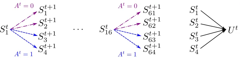
We consider data from the following class of generative models, as illustrated in Figure

2.3:

S1_∼Normal₆₄(0, 0.25I64); A1, . . . ,AT ∼i.i.d.Bernoulli(0.5);

S₄t_i+₋1₃,S₄t_i+₋1₂∼i.i.d.Normal

(1−At)g(S_it), 0.01(1−At) +0.25At ;

S₄t_i+₋1₁,S₄t_i+1∼i.i.d.Normal

Atg(S_it), 0.01At+0.25(1₋At) ;

Ut ∼Normal{(1₋At)[2_{g(S₁t) +g(S₂t)} − {g(S₃t) +g(S₄t)}]

+At[2{g(S₃t) +g(S₄t)} − {g(S₁t) +g(S₂t)}], 0.01};

fori =1, 2, . . . , 16.

Figure 2.3 Relationship betweenSt andYt+1in the generative model, which depends on the

action. First 16 variables determine the next state. First 4 variables determine the utility.

The above class of models is indexed byg :R→Rwhich we vary across the following maps: identityg(u) =u, truncated quadraticg(u) =min{u2_{, 3}_}_{, and truncated exponential}

g(u) =min_{eu_{, 3}_}_{, where the truncation is used to keep all variables of relatively the same} scale across time points. Additionally, we add 3 types of noise variables, each taking up

about1₃ of total noises added:

(i) dependent noise variablesDt

j , which are generated the same way as above except

(38)

time point; and

(iii) constantsCt

l , which are sampled independently from Normal(0, 0.25)att =1 and remain constant over time.

More precisely, letm be the total number of noise variables, then

D_j1,W_k1,C_l1∼i.i.d.Normal(0, 0.25);

D₄t_i+₋1₃,D₄t_i+₋1₂∼i.i.d.Normal

(1−At)g(D_it), 0.01(1−At) +0.25At ;

D₄t_i+₋1₁,D₄t_i+1∼i.i.d.Normal

Atg(D_it), 0.01At +0.25(1₋At) ;

W_kt ∼i.i.d.Normal(0, 0.25);Clt =C

1

l ;

forj =1, 2, . . . ,bm/3c;k =1, 2, . . . ,dm/3e;l =1, 2, . . . ,dm/3e.

It can be seen that the first 16 variables, the first 4 variables, and{g(S₁t),g(S₂t),g(S₃t)+g(S₄t)}ü all induce a sufficient MDP. the foregoing class of models is designed to evaluate the ability

of the proposed method to identify low-dimensional and potentially nonlinear features

of the state in the presence of action-dependent transitions and various noises. For each

Monte Carlo replication, we samplen=30 i.i.d. trajectories of lengthT =90 from the above generative model.

The results based on 500 Monte Carlo replications are reported in Table 2.1 - 2.3. In

addition to reporting the marginal mean outcome under the policy estimated using

Q-learning with both function approximations, we also report: (nVar) the number of selected

variables; and (nDim) the dimension of the feature map. It can be seen that

(i) ADNN produces substantially smaller nVar and nDim compared with PCA or tNN in

all cases;

(39)

(iii) when fed into the Q-learning algorithm, ADNN leads to considerably better marginal

mean outcome than PCA and the original states with non-linear models;

(iv) ADNN is able to construct features suitable for Q-learning with linear function

approx-imation even when the utility function and transition between states are non-linear;

(v) even when Q-function is a flexible function approximator like neural nets, marginal

mean outcome could still be poor when input features are high dimensional (Table

2.2), suggesting the necessity of efficient dimension reduction.

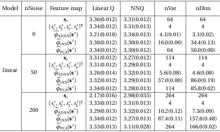
Table 2.1 Comparison of feature map estimators under linear transition across different

number-s of noinumber-se variablenumber-s (nNoinumber-se) in termnumber-s of: marginal mean outcome unumber-sing Q-learning with linear function approximation (Linear Q); Q-learning with neural network function approximation (NN Q); the number of selected variables (nVar); and the dimension of the feature map (nDim)

Model nNoise Feature map Linear Q NNQ nVar nDim

linear

0

st 3.36(0.012) 3.31(0.012) 64 64

(st

1,s

t

2,s

t

3,s

t

4)ü 3.34(0.012) 3.31(0.013) 4 4

Ò

φADNN(st) 3.21(0.018) 3.34(0.013) 4.1(0.01) 3.1(0.02) Ò

φtNN(st₎ _3.38(0.012) _3.30(0.012) _16.0(0.00) _34.4(0.13) Ò

φPCA(st₎ _3.34(0.012) _3.30(0.012) ₆₄ _50.0(0.00)

50

s_t 3.31(0.012) 3.27(0.012) 114 114

(st

1,s

t

2,s

t

3,s

t

4)ü 3.31(0.012) 3.29(0.013) 4 4

Ò

φADNN(st₎ _3.26(0.014) _3.32(0.013) _5.6(0.08) _4.6(0.08) Ò

φtNN(st) 3.32(0.012) 3.29(0.013) 37.0(0.00) 86.0(0.19) Ò

φPCA(st₎ _3.34(0.012) _3.28(0.013) ₁₁₄ _85.8(0.02)

200

st 2.17(0.016) 2.98(0.035) 264 264

(st

1,s

t

2,s

t

3,s

t

4)ü 3.33(0.012) 3.31(0.013) 4 4

Ò

φADNN(st₎ _3.29(0.013) _3.32(0.012) _10.2(0.12) _7.5(0.09) Ò

φtNN(st₎ _3.34(0.012) _3.27(0.013) _87.4(0.11) _157.8(0.48) Ò

Sufficient Markov Decision Processes.

ABSTRACT

DEDICATION

BIOGRAPHY

ACKNOWLEDGEMENTS

TABLE OF CONTENTS

LIST OF TABLES

LIST OF FIGURES

CHAPTER 1

THEORETICAL FRAMEWORK OF

SUFFICIENT MARKOV DECISION

PROCESSES

1.1

Introduction

1.2

Setup and Notation

1.3

Theoretical Results

1.3.1

Variable Screening

1.4

Discussion

CHAPTER 2

CONSTRUCTING SUFFICIENT MARKOV

DECISION PROCESSES WITH

ALTERNATING DEEP NEURAL

NETWORKS

2.1

Introduction

2.2

Method

2.3

Simulation Experiments