Statistical method for testing the neutral mutation hypothesis by DNA polymorphism.

(1)

Copyright 0 1989 by the Genetics Society of America

Statistical Method for Testing the Neutral Mutation Hypothesis by DNA

Polymorphism

Fumio Tajima

Department of Biology, Kyushu University, Fukuoka 812, Japan

Manuscript received February 13, 1989 Accepted for publication July 14, 1989

ABSTRACT

The relationship between the two estimates of genetic variation at the DNA level, namely the number of segregating sites and the average number of nucleotide differences estimated from pairwise comparison, is investigated. It is found that the correlation between these two estimates is large when the sample size is small, and decreases slowly as the sample size increases. Using the relationship obtained, a statistical method for testing the neutral mutation hypothesis is developed. This method needs only the data of DNA polymorphism, namely the genetic variation within population at the DNA level. A simple method of computer simulation, that was used in order to obtain the distribution of a new statistic developed, is also presented. Applying this statistical method to the five regions of DNA sequences in Drosophila melanogaster, it is found that large insertion/deletion (>lo0 bp) is deleterious. It i s suggested that the natural selection against large insertion/deletion is so weak that a large amount of variation is maintained in a population.

A

large amount of genetic variation is maintained in natural populations. Information about this variation at the DNA level can be obtained from DNA sequencing or restriction enzyme technique. WATTER- SON (1975) has shown under the neutral mutation model (KIMURA 1968,1983) that the expectation and variance of the number ( S ) of segregating (or poly- morphic) sites in the sample are given by

E ( S ) = u ~ M , (1)

and

V(S) = a l M

+

a2M2, (2)

respectively, where M = 4Nu, N is effective population size, u is the mutation rate per generation per DNA sequence under investigation,

n-l 1

a

n--l 1

a1 =

E

7 , (3)

a 2 =

E

2,

(4)

and n is the sample size (the number of DNA sequences studied), so that M can be estimated from

i= 1

A S

a1

M =

-.

₍₅₎

It should be noted that S itself is not a good statistic for estimating the DNA polymorphism, since S de- pends on the sample size. On the other hand, TAJIMA (1 983) has shown under the neutral mutation model that the expectation and variance of the average num-

Genetics 123: 585-595 (November, 1989)

ber

(i)

of (pairwise) nucleotide differences between the DNA sequences examined are given by

E ( i ) = M , (6)

and

V ( i ) = blM

+

b2M2,

(7)

respectively, where

bl =

n + l

3(n

-

1)’

and

2(n2

+

n

+

3)

9n(n

-

1) ’ (9)

b2 =

This number

(i)

not only has clear biological mean- ings, but also gives the estimate of M directly.

(2)

gating sites may not be the same as the average number of nucleotide differences which also is the estimate of M.

In this paper I shall investigate the relationship between the number of segregating sites and the average number of nucleotide differences under the neutral mutation model. Using this relationship obtained, I shall also present a statistical method for testing the neutral mutation hypothesis.

RELATIONSHIP BETWEEN THE NUMBER OF

SEGREGATING SITES AND T H E AVERAGE NUMBER OF NUCLEOTIDE DIFFERENCES

Assumption: In this paper we consider a random mating population of N diploid individuals and assume that there is no selection and no recombination between DNA sequences. We also assume that the number of sites on a DNA sequence is so large that a newly arisen mutation takes place at a site different from the sites where the previous mutations have occurred [infinite site model (KIMURA 1969)l. Under these as- sumptions the expectation and variance of the number of segregating sites are given by (1) and

(2),

and the expectation and variance of the average number of nucleotide differences are given by (6) and

(7).

Covariance between the number of segregating sites and the average number of nucleotide differ- ences: If we denote the number of nucleotide differences between the ith and jth DNA sequences by

kj,

the average number of (pairwise) nucleotide differences between the DNA sequences sampled is given by

E

k,

k =

A i<j

($

'

(10)

where n is the number of DNA sequences sampled. Incidentally can also be estimated from

S

k^

= hi, (1 1)

where S is the number of segregating sites, and hi is the unbiased estimate of nucleotide diversity (or het- erozygosity) for the ith segregating site, which is given

i= 1

by

n ( l - Z x 3 j )

hi =

n - 1 , (12)

where xji is the sample frequency of the jth allelic nucleotide in the ith segregating site. When the sample size (n) is large, (1 1) is more practical than (1 0).

If we use (1 0), the covariance between the number

of segregating sites and the average number of nucleotide differences can be given by

Cov(S,

i )

= COV(S, k,). (13)

This covariance can be obtained from the genealogical relationship of DNA sequences.

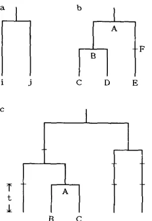
When n is 2, S is equal to

k,

(Figure la), so that Cov(S, kq) = V ( k j ) = V ( S ) . From

(2)

V ( S ) is equal to M

+

M 2 . Therefore, we have

Cov(S,

I)

= M

+

M2. (14)

The genealogical relationship when n is 3 is shown in Figure lb. In this case there are two possible common ancestors (namely A and B ) between the two

DNA sequences which are randomly chosen from the three DNA sequences. Since B is the common ancestor when C and D are chosen, and A is the common ancestor when C and E , or D and E are chosen, the probability that B is the common ancestor is %, and that of A is 2/9. Therefore, the covariance is given by

cov(S,

i )

= '/s cov(S, k C D )

+

?h

cov(s, kCE), where S = ~ B F

+

~ B C

+

k g D

+

R E F . If we notice that the distributions of k B , k B D , and kEF are the same, we can get

cov(S, kCE) = v(kBJ7)

+

cov(S, kCJJ).

TAJIMA (1 983) has shown that

V ( & ) = M

+

M2, v ( k B c ) = M/6

+

M2/36,

COV(~BC, ~ B D ) = M2/36,

so that we have

cov(S, k m ) = V ( ~ C D )

+

~COV(~BC, ~ B D )

2 V ( k ~ c )

+

~ C O V ( ~ B C , ~ B D ) = M/3

+

M2/6.

Using these equations, we obtain

cov(S, ff) ?h v ( k B F )

+

cov(S, kCD)

(1 5 ) = M

+

5/6 M2.

Next, we consider the case where the number of

DNA sequences sampled is more than 3. n DNA

sequences take place when one of n

-

1 DNA sequences bifurcates. Suppose that such a bifurcation occurred at point A in Figure IC, and that its descend- ants are B and C. Then the covariance between S and

is given by

(3)

Test of Neutral M 'utation Hypothesis

Following TAJIMA (1983), we have

587

i j

C

C D E

M M

=-+{-I

2

B C

FIGURE 1 .-(a) Expected genealogical relationship when two

DNA sequences are sampled from a population. (b) Expected ge-

nealogical relationship when three DNA sequences are sampled from a population. (c) One example of the genealogical relationship among five DNA sequences sampled from a population.

where kG is not equal to kBc. Using the same method as the above, we can have

cov(S, KBC) = v(kBC)

+

2(n

-

2)cov(kAB, k A C ) , (17)

and

Cov(S,

k,)

= Cov(S*,

**k*)**

+

V(kBc)

(1 8)

+

2(n

-

2)Cov(k~t3, ~ A C ) , where S* and

&*

are the number of segregating sites and the average number of nucleotide differences for n

-

1 DNA sequences, respectively. Substituting

(17)

and (1 8) into (1 6), we have

Cov(S, I;) = (n

+

l)(n

-

n(n

-

1)

2,

COV(S*,

**i * )**

₍₁₉₎

+

v ( k B C )

+

2(n

-

2)cov(kAB, kAC). Following TAJIMA (1 983), we can obtain V(kBc) and C o v ( k ~ ~ , kAc). HUDSON (1 983) and TAJIMA (1 983) have shown that the probability that n DNA sequences randomly sampled from a population are derived from n

-

1 DNA sequences t generations ago and the divergence took place t - 1 generations ago (see t in Figure IC) is given by

where

Substituting

(2

1) and (22) into (19), we have

COV(S,

i )

= (n

+

l)(n

-

2) COV(S

*,

**i * )**

n(n

-

1) (23) _. _,

+

2M

₊

2M2 n(n

-

1) n(n

-

Since Cov(S, I;) is M

+

M2 when n is 2, we finally have

As n increases, (24) approaches

COV,t(S,

i )

= M

+

% M 2 . ( 2 5 )

We call this covariance the stochastic covariance. T h e sampling covariance is given by

COV,(S,

i)

= COV(S,

i)

-

COV,@,

i)

=- M2. (26)

T h e correlation coefficient ( r ) between S and

k^

is defined as

1 n

COV(S, I;)

r=7*

_V(S)V(k)

(27)

Numerical computations show that this correlation coefficient is large when the sample size (n) is small, and decreases slowly as the sample size increases.

(4)

Let us define

d

as

where a l is given by (3). Then, the expectation of

d

is

0 and the variance of

d

is given by

where V ( i ) , V(S), and Cov(S,

I )

are given by

(7),

(2),

and (24), respectively. Substituting these quantities

into (29), we have

V(d)

= clM

+

c2M2, (30)

where

and

These equations indicate that, unlike the other variances such as the variances of S and

I ,

the variance of

d

increases as n increases and reaches to the asymp- totic value which is identical with the variance of ff.

STATISTICAL METHOD FOR T E S T I N G T H E NEUTRAL MUTATION HYPOTHESIS

Estimating d and V ( d ) : In the previous section we have obtained the variance of

d.

Formula (30), however, cannot be used directly for estimating the variance of

d,

since we do not know M. M can be estimated from S/al or

i.

We notice from (2) and 17) that the variance of S / a l is smaller than that of

K

when n is larger than 3. Therefore, S / a l should be used for estimating M when the neutral mutation hypothesis is correct. Since we assume the neutral mutation hypothesis as a null hypothesis, M is estimated by S/al [see (5)]. @/a1)’, however, cannot be used for estimating M 2 , since the expectation of S2 is given by

E(S2) = V(S)

+

(E(S)12 ₍₃₃₎

= a l M

+

(a:

+

a2)M2,

which is not equal to aTM2. As E ( S 2 )

-

E ( S ) =

(a: + a2)M2, M 2 can be estimated by

S(S

-

1) a:

+

a2’ Therefore, we can estimate

V(d)

by

(34)

?(d)

= elS

+

e d ( S

-

l), (35)

where

el = -,

a1 c1

and

New statistic ( D ) : In order to conduct the statistical test, the following statistic is proposed:

k.

*

-

s

d

D = r - J

-

a1

* (38)

v

( 4

elS

+

e$(S

-

1)

where a l , e l , and e2 are given by (3), (36), and (37).

Then, the mean and variance of D are approxi- mately 0 and 1, respectively. If we know the distribution of D , then we can use D in testing the neutral mutation hypothesis. For this purpose the following computer simulation was conducted.

Computer simulation: First, genealogical relationships of DNA sequences are generated as follows. When there are n DNA sequences, we randomly choose two DNA sequences among n DNA sequences, combine these two DNA sequences, and obtain new

n

-

1 DNA sequences. Figure 2 shows one example of this process. In the case of 5 DNA sequences (A, B, C,

D ,

and E ) , if B and C are chosen, we obtain new four DNA sequences (A, BC, D , and E ) . Next, three DNA sequences (A, BC, and DE) are obtained if D and E are chosen. Furthermore, if A and BC are chosen, then we obtain the genealogical relationship of five DNA sequences shown in Figure 2. In this way we can obtain many genealogical relationships of n DNA sequences.

Next, we generate the number of mutations in each branch. Let

Si,

be the number of mutations in the ith branch among n branches between n DNA sequences and n

-

1 DNA sequences (Figure 2), and S , be the total number of mutations in n branches, namely

n

s,

=

st,.

₍₃₉₎

I= 1

Then, S , follows the geometric distribution,

P ( S n ) = p n ( l

-

pn)’n? (40)

where

1

M 1

+-

n - 1

pn

= (41)

(see WATTERSON, 1975). T h e joint probability of SI,, S2,,

. .

.

, and S,, for a given value of S , is given by

i= 1

(5)

Test of Neutral Mutation Hypothesis 589

using (1 l ) , so that we have

A B C D E

s12 s22

A B C

’13 ’23

s34 s44

’25 s35

FIGURE 2.-One example of the genealogical relationship among five DNA sequences used for explaining the process of computer simulation.

obtained according to (42). In this way we can get the numbers of mutations in all branches for each genealogical relationship.

Once we have a set of data, we can easily compute the number of segregating sites (S = S 2

+

S S

+

.

+

S,) and the average number of nucleotide differences

(i).

Then, we compute D by (38).

I n this simulation we used three values of M (1, IO,

and loo), and four values of n ( 5 , 10, 20, and 30). In

each case we repeated 1000 times. T h e mean and variance of D in each case are shown in Table 1 , and the distribution of D is given in Figure 3. As expected, we can see that the mean of D is nearly zero, although it is negative. T h e variance of D, however, is smaller than 1, especially when M is large. When we conduct a statistical test, this property is not necessarily harm- ful since it reduces the possibility of rejection. From Figure 3, we can see that the distribution of D is not symmetrical, so that it does not follow the unit normal distribution. For the significant test of neutral mutation hypothesis, however, we can use the unit normal distribution as seen in Table 1. For example, the probability that D is larger than

2

is 0.023 if the unit normal distribution is used. T h e result obtained from this simulation shows that only in the case of M = 1

and n = 30 the proportion of D

>

2

(0.029) is larger than 0.023.

One of the problems in using the unit normal distribution is that the actual values of D can take only limited values. T h e minimum value of d is obtained when the frequencies of two allelic nucleotides are

l / n and 1

-

l f n in every segregating site. In this case we obtain

2 n

imin

=

-

s,

(43)

T h e minimum value of D is obtained when S is infi- nitely large. From (38) we can obtain

2 1

” -

T h e maximum value can be obtained in the same way as the above, which is given by

n

_{- -}

1

when n is an even number, or

n + l 1

”

-when n is an odd number. One of the basic distributions which often appear in biological study is a beta distribution. Let us consider the beta distribution an approximate distribution of D . Since the mean and variance of D are assumed to be 0 and 1, the beta distribution can be written as probability density func- tion:

where

( 1

+

ab)b

a = -

b - u ’

(1

+

ab)a

p =

’

a = Dmin, and b = D,,,.

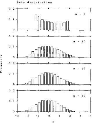
Figure

4

shows the beta distribution, which well agrees with the actual distribution of D obtained from the computer simulation. Table 1 also shows the beta distribution. From this table we can see that the beta distribution fits the actual distribution better than the normal distribution. Because of the above reason, the beta distribution is recommended for testing the neutral mutation hypothesis.

(6)

TABLE 1

Comparisons of the distribution of D obtained by computer simulation with the normal and beta distributions

D

n M -3"2 - 2 - - 1 - 1 - 0 0 - 1 1 - 2 2 - 3 3 - 4 Mean Variance

5

10

20

30

1 0.154 0.393

10 0.162 0.389

100 0.133 0.416

Beta 0.222 0.324

1 0.000 0.226 0.287

10 0.007 0.179 0.340

100 0.002 0.165 0.386

Beta 0.003 0.177 0.336

1 0.004 0.212 0.32 1

10 0.005 0.150 0.395

100 0.004 0.149 0.403

Beta 0.01 1 0.161 0.342

1 0.002 0.171 0.354

10 0.01 1 0.161 0.410

100 0.007 0.140 0.423

Beta 0.012 0.157 0.345

Normal 0.021 0.136 0.341

0.181 0.272 0.260 0.189 0.279 0.179 0.236 0.218

0.313 0.164 0.011

0.338 0.128 0.008

0.325 0.117 0.005

0.304 0.156 0.023

0.296 0.153 0.014 0.000

0.316 0.117 0.017 0.000

0.327 0.114 0.003 0.000

0.315 0.146 0.025 0.000

0.298 0.145 0.028 0.001

0.313 0.096 0.009 0.000

0.321 0.100 0.009 0.000

0.317 0.142 0.026 0.001

0.341 0.136 0.021 0.001

-0.007 0.949

-0.0 16 0.813

-0.025 0.755

0 1

-0.036 0.941

-0.072 0.851

-0.104 0.755

0 1

-0.050 0.959

-0.074 0.839

-0.080 0.724

0 1

-0.002 0.977

-0.154 0.801

-0.110 0.751

0 1

n = 7 0

0 1 0. I

0 0

1 2 ! 0 ! 2 1 4 - 3 - 2 - 1 0 1 2 3 4 - 3 - 2 I O I 2 7 4

FIGURE 3.-Distributions of D obtained from computer simulation.

DISTRIBUTION OF NUCLEOTIDE FREQUENCY ber of nucleotides with frequency i / n in a sample of n

IN T H E SAMPLE DNA sequences is given by

In this section we investigate the distribution of nucleotide frequency in the sample. Consider a given site. If we use the infinite allele model, then the expected number of nucleotides with frequency

( p ,

p

+

d p ) in a population is given by

(KIMURA and CROW 1964), where p is the mutation

(7)

Test of Neutral Mutation Hypothesis 59 1

0 . 2

n = 1 0 0 1

2 0

D 0 2

n 2 0

y. 0 1 0 0 . 2

" = 3 0

0 1

0

- 3 2 - 1 0 1 2 3 4 D

FIGURE 4,"Expected distributions of D obtained by assuming that D follows beta distribution.

n

-

1. We now assume that there are m sites on the DNA sequence. Then the expected number of nucleotides whose frequency is i / n in a sample of n DNA sequences with m sites can be obtained if we assume 4Npm = 4Nu = M , p + 0, and m 4 m, and is given

by

G,(i) = M

(t

7

+

-

. ti ))

when 1 5 i

5

n

-

1. If we use S/al instead of M , then we have

Incidentally the sum of G,(i) for i = 1 to n

-

1 is 2S,

since there are two allelic nucleotides in each segregating site. Using (51), we can compare the observed distribution of nucleotide frequency with the expected one, although we cannot conduct a significant test by using this comparison.

NUMERICAL EXAMPLE

AQUADRO and GREENBERG (1983) studied a sequence of about 900 nucleotide pairs of the human mitochondrial DNA for seven individuals (n =

7).

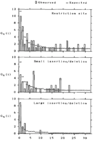
T h e number of segregating sites (S) is 45, and the average number of nucleotide differences (ff) estimated was 15.38. In this case the values of a ] , e l , and e2 are 2.4500, 0.01481, and 0.004784, respectively. Using (38), we obtain D = -0.9382, which is not significantly different from 0 (Table 2), s o that we conclude that the neutral mutation hypothesis can explain the DNA polymorphism of human mitochondrial DNA.

Incidentally, the distribution of nucleotide frequency in the sample is shown in Figure 5, which indicates that the numbers of nucleotides with frequencies '/7 and 6/7 are larger than the expected ones.

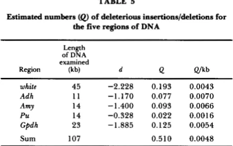
Miyashita and Langley (1988) examined a 45-kb region of the white locus on the X chromosome in Drosofhila melanogaster, using 64 X chromosome lines

(n = 64) with six 6-cutter and ten 4-cutter restriction enzymes. They classified the DNA polymorphisms into three groups, namely restriction site polymorphism, small insertion/deletion (<lo0 bp) polymorphism, and large insertion/deletion (>lo0 bp) polymorphism. As long as the infinite site mutation model is applicable, we can use this method. In the cases of restriction site and insertion/deletion, there are many sites where mutations can take place. Therefore, we can apply the present test to these cases. Unlike the mitochondrial DNA, however, some recombination may occur on the nuclear DNA. In this case the actual variance of d is smaller than that of (30), so that the actual value of D takes more extreme value than that estimated by (38). Because of this, the present method might be conservative when the nuclear DNA is ana- lysed. The result of the present test is shown in Table 3. Significant deviation of

D

from 0 is observed (P

<

0.05) only in the case of large insertion/deletion polymorphism, so that we can reject the null hypothesis that all the large insertion/deletion polymorphisms are maintained without selection at the 5% level.

One of the possible explanations of this is that the large insertions/deletions are deleterious so that they are maintained with low frequency. This can be seen in Figure 6. In this figure only the numbers of segregating sites whose frequencies are less than or equal to 32/64 are shown, since the number of segregating

sites with frequency i / n is equal to that of ( n

-

i ) / n . From this figure we can see that the numbers of segregating sites with low frequencies are much larger than the expected ones.

Another possible explanation is that the population does not reach to the equilibrium yet. For example, if

a population experienced a bottleneck recently, many sites with low frequency might be observed. There- fore, D is expected to be negative. Since the values of

D observed in the cases of restriction site and small insertion/deletion polymorphisms are positive, the bottleneck effect cannot explain the result that the value of

D

observed in the case of large insertion/ deletion is significantly smaller than 0.

(8)

F. Tajima

TABLE 2

Confidence limit of D obtained by assuming the beta distribution

Confidence limit of D

n 90% 95% 99% 99.9%

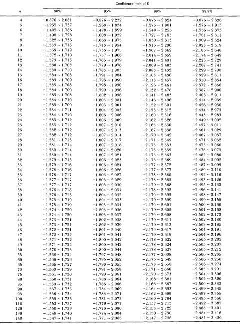
4 5 6 7 8 9 10 11 12 13 14 15 16 17 18 19 20 21 22 23 24 25 26 27 28 29 30 31 32 33 34 35 36 37 38 39 40 41 42 43 44 45 46 47 48 49 50 55 60 65 70 75 80 85 90 95 100 110 120 130 140

-0.876

-

2.081 -1.255

-

1.737

-

1.405

-

1.786 -1.498

-

I .728 -1.522

-

1.736 -1.553

-

1.715 -1.559

-

1.719 -1.572

-

1.710 -1.573

-

1.713 -1.580

-

1.708 -1.580

-

1.710 -1.584

-

1.708 -1.583

-

1.709 -1.585

-

1.708 -1.584

-

1.709 -1.585

-

1.708 -1.584

-

1.710 -1.585

-

1.709 -1.584

-

1.711 -1.584

-

1.710 -1.583

-

1.712 -1.583

-

1.712 -1.582

-

1.712 -1.582

-

1.712 -1.581

-

1.713 -1.581

-

1.714 -1.580

-

1.714 -1.580

-

1.714 -1.579

-

1.715 -1.579

-

1.716 -1.578

-

1.716 -1.578

-

1.717 -1.577

-

1.717 -1.577

-

1.717 -1.576

-

1.718 -1.576

-

1.718 -1.575

-

1.719 -1.575

-

1.719 -1.574

-

1.720 -1.574

-

1.720 -1.573

-

1.721 -1.573

-

1.721 -1.572

-

1.721 -1.572

-

1.722 -1.571

-

1.722 -1.571

-

1.722 -1.570

-

1.723 -1.568

-

1.724

-

1.566

-

1.726 -1.565

-

1.727 -1.563

-

1.729 -1.561

-

1.730 -1.560

-

1.731 -1.559

-

1.732 -1.557

-

1.733 -1.556

-

1.734 -1.555

-

1.735 -1.552

-

1.737 -1.550

-

1.739 -1.549

-

1.740 -1.547

-

1.741

-0.876

-

2.232 -1.269

-

1.834 -1.478

-

1.999 - 1.608

-

1.932 -1.663

-

1.975 -1.713

-

1.954 -1.733

-

1.975 -1.757

-

1.966 - 1.765

-

1.979 -1.779

-

1.976 -1.783

-

1.985 -1.791

-

1.984 -1.793

-

1.990 -1.798

-

1.990 -1.799

-

1.996 -1.802

-

1.996 -1.803

-

2.001 -1.805

-

2.001 -1.804

-

2.005 -1.806

-

2.006 -1.806

-

2.009 -1.807

-

2.010 -1.807

-

2.013 -1.807

-

2.014 -1.807

-

2.017 -1.807

-

2.018 -1.807

-

2.020 -1.807

-

2.021 -1.806 - 2.023 -1.806

-

2.024 -1.806

-

2.026 -1.806

-

2.027 -1.805

-

2.029 -1.805

-

2.030 -1.804

-

2.031 -1.804

-

2.032 -1.804

-

2.033 -1.803

-

2.034 -1.803

-

2.036 -1.803

-

2.037 -1.802

-

2.038 -1.802 -, 2.039

-1,801

-

2.040 -1.801

-

2.041

- 1 .SO0

-

2.042 -1.800

-

2.042 -1.800

-

2.044 -1.797

-

2.048 -1.795

-

2.052 -1.793

-

2.055 -1.791

-

2.058 -1.790

-

2.061

-

1.788 5 2.064

-1.786

-

2.066

-

1.784

-

2.069 -1.783

-

2.071 -1.781

-

2.073 -1.779

-

2.077 -1.776

-

2.080 -1.774

-

2.084 -1.771

-

2.086

-0.876

-

2.324 -1.275

-

1.901 -1.540

-

2.255 -1.721

-

2.185 -1.830

-

2.313 -1.916

-

2.296 -1.967

-

2.362 -2.014

-

2.359 -2.041

-

2.401 -2.069

-

2.403 -2.085

-

2.432 -2.103

-

2.436 -2.1 13

-

2.457 -2.126

-

2.461 -2.132

-

2.478 -2.141

-

2.483 -2.146

-

2.496 -2.152

-

2.501 -2.153

-

2.512 -2.160

-

2.516 -2.162

-

2.526 -2.165

-

2.530 -2.167

-

2.538 -2.170

-

2.542 -2.171

-

2.549 -2.173

-

2.553 -2.173

-

2.559 -2.175

-

2.563 -2.175

-

2.569 -2.177

-

2.572 -2.177

-

2.577 -2.178

-

2.580 -2.178

-

2.585 -2.179

-

2.588 -2.178

-

2.592 -2.179

-

2.595 -2.179

-

2.599 -2.179

-

2.601 -2.179

-

2.605 -2.179

-

2.608 -2.179

-

2.611 -2.179

-

2.613 -2.179

-

2.617 -2.179

-

2.619 -2.178

-

2.622 -2.178

-

2.624 -2.178

-

2.627 -2.177

-

2.638 -2.175

-

2.649 -2.173

-

2.658 -2.171

-

2.666 -2.170

-

2.673 -2.168

-

2.681 -2.166

-

2.687 -2.164

-

2.693 -2.162

-

2.699 -2.160

-

2.704 -2.157

-

2.713 -2.153

-

2.722 -2.150

-

2.730 -2.147

-

2.736

(9)

Test of Neutral Mutation Hypothesis 593

TABLE 2-Continued

~~

Confidence limit of D

n 90% 95% 99% 99.9%

150 -1.545

-

1.743 -1.769

-

2.089 -2.144

-

2.743 -2.477

-

3.443 175 -1.542

-

1.746 -1.765

-

2.095 -2.138

-

2.757 -2.470

-

3.470 200

250 300 350 400 450 500 600 800 1000

-1.539

-

1.748 -1.534

-

1.752 -1.530

-

1.755 -1.526

-

1.757 -1.523

-

1.759 -1.521

-

1.761 -1.519

-

1.763 -1.515

-

1.765 -1.510

-

1.769 -1.505

-

1.772

-1.760

-

2.100 -1.754

-

2.107 -1.748

-

2.114 -1 .744- 2.119 -1.740

-

2.123 -1.737

-

2.127 -1.734

-

2.130 -1.728

-

2.135 -1.721

-

2.143 -1.715

-

2.150

-2.132

-

2.768 -2.122

-

2.787 -2.114

-

2.802 -2.107

-

2.814 -2.101

-

2.824 -2.096

-

2.833 -2.092

-

2.840 -2.084

-

2.853 -2.072

-

2.873 -2.062

-

2.887

-2.462

-

3.492 -2.449

-

3.529 -2.439

-

3.558 -2.430

-

3.581 -2.422

-

3.600 -2.415

-

3.617 -2.409

-

3.632 -2.398

-

3.657 -2.382

-

3.694 -2.369

-

3.722

I 2 3 4 5 6

FIGURE 5.-Observed and expected distributions of the number of allelic nucleotides for human mitochondrial DNA. The observed distribution was obtained from AQUADRO and GREENBERG (1 983), and the expected distribution was obtained by assuming the neutral mutation model.

of D in the case of restriction site polymorphism does not show a significant deviation from 0, but that of insertion/deletion (>300 bp) polymorphism shows a significant deviation in the case of Amy. If we pool the data of four regions of DNA, the deviation of D from 0 becomes highly significant (P

<

0.01). In this case the value of D was obtained by the sum of the values of d divided by the square root of the sum of the estimated variances of d , since these four regions can be assumed to be unlinked. The distribution of the sum of independent random variables approaches the normal distribution as the number of variables increases, and the computer simulation conducted ear- lier indicates that the distribution of D is not far from the normal distribution. Because of these reasons, in order to find the confidence limit of D , we can use the normal distribution when several regions of DNA are used. At any rate, if we apply the unit normal distribution in this case, the deviation of D from 0 is highly significant (P

<

O.Ol), so that the neutral mutation hypothesis is rejected.

DISCUSSION

In this paper we have obtained a statistical method for testing the neutral mutation hypothesis by using DNA polymorphism. Unlike HUDSON, KREITMAN and

TABLE 3

Estimates of D for the three groups of polymorphisms in the

white locus in D. melanogaster

Type of

polymorphism S k ^ D

Restriction site 53 11.92 0.2128 (NS) Small insertion/deletion 40 10.02 0.6075 (NS)

Large insertion/deletion I5 0.94 -2.0709 (P 0.05)

Data from MIYASHITA and LANGLEY (1988). NS, not Significant (P > 0.1).

ACUADE (1 987) where not only DNA polymorphism data but also between species divergence data are necessary, only DNA polymorphism data are needed to use this method. In many cases only DNA polymorphism data are available, so that this method might be useful. When we apply this method, however, some caution is necessary. (1) The DNA sequences applied to this method must be a random sample from a population. (2) We must take into consideration whether the population is at equilibrium or not. For example, as shown in the NUMERICAL EXAMPLE section, a negative value of D can also be obtained if the population experienced a bottleneck recently. In this case a comparison between different kinds of DNA polymorphisms such as a comparison between nucleotide and insertion/deletion polymorphisms may help our interpretation, since a bottleneck affects all kinds of DNA polymorphisms. (3) If a selectively neutral site is linked to a site at which natural selection is operating, then the value of D for the neutral site might be affected by the selected site. [For the coalescent process for a neutral site which is linked to a selected site, see KAPLAN, DARDEN and HUDSON ( 1 988) and HUDSON and KAPLAN (1988).]

In the NUMERICAL EXAMPLE section, we analyzed the five regions of DNA sequences, white, Adh, Amy,

(10)

F. Tajima

6 G,(il

4

2

0

1 0

', S m a l l i n r e r t l o n / d e l e t i o n

8

0 5 1 0 1 5 2 0 2 5 3 0

FIGURE 6.-Observed and expected frequency spectrums of pol- ymorphic variation in the white locus region of D. melanogaster. The

observed spectrums were obtained from MIYASHITA and LANGLEY (1988), and the expected spectrums were obtained by assuming the neutral mutation model.

Under the neutral mutation hypothesis, the probability that D is positive is less than !h (see Table l), so

that the probability that all the five D values are positive is less than l/~z. Therefore, there may k c a site at which natural selection, which increases the genetic variation, is operating. Among the five values of D, the value of D for Adh is quite large, although it is not significantly different from 0. The exceptionally high level of variation was observed in the Adh coding region by KREITMAN and A G U A D ~ ( 1 986), so that the large D value may be explained by natural selection.

Negative values of D were observed in the case of large insertion/deletion for all five regions of DNA. [The length of insertion/deletion in T. TAKANO, S .

KUSAKABE and T. MUKAI (in preparation) is longer

than 300 bp, so that we call it large insertion/deletion according to MIYASHITA and LANGLEY (1 988).] Under the deleterious mutation model, we can estimate the total number of deleterious mutants per DNA sequence (or per genome).

Let qi be the frequency of deleterious nucleotide in the ith deleterious site in a population. If we consider the deleterious site as well as the neutral site, then the expectation of the number of segregating sites for a sample of n DNA sequences is given by

E ( S ) = U ~ M

+

2

[ I

-

9:

-

(1

-

qi)"1.

If we assume that qi is very small, then E ( S ) is approx- imately given by

E ( S ) = a l M

+

n

x

q i . (52)

TABLE 4

Estimates of D for four regions of DNA in D. melanogaster

Restriction site Insertion/deletion

Region S k^ D S k ^ D

Adh 4 1.39 _{1.52O(Ns) 10 0.82 - 1 . 5 3 7 ( ~ S )}

Amy 7 1.74 0 . 5 9 9 * ( ~ ~ ) 10 0.59 -1.839 ( P c 0 . 0 5 )

Pu 6 _{1.25 0.108(Ns)} 2 0.07 -1.305 (NS) Gpdh 18 4.27 0.559 (Ns) 15 1.10 -1.784(P<O.l)

Sum 35 8.64 1 . 1 1 1 (NS) 37 2.58 -3.127 (P<O.Ol)

Data from T. TAKANO, S. KUSAKABE and T. MUKAI (in prepa- ration). NS, not significant ( P > 0.1).

On the other hand, the expectation of the average number of nucleotide differences is given by

= M

+

2

2941

-

qi)

(53) = M + 2 x q i .

If we define d by (28) as before, then the expectation of d becomes

(54)

Therefore, the total number of deleterious mutants per DNA sequence

(E

4;)

can be estimated by

d

Q =

.

"

n

"

2

(55)

a1

(11)

Test of Neutral Mutation Hypothesis 595

TABLE 5

Estimated numbers

(0

of deleterious insertions/deletions for the five regions of DNA

Length of DNA examined

Region (kb) d 4 Q/kb

white 45 -2.228 0.193 0.0043

Adh 11 -1.170 0.077 0.0070

Amy 14 -1.400 0.093 0.0066

Pu 14 -0.328 0.022 0.0016

Gpdh 23 -1.885 0.125 0.0054

Sum 107 0.510 0.0048

Data for white from MIYASHITA and LANGLEY (1988). Data for the others from T. TAKANO, S. KUSAKABE and T. MUKAI (in preparation).

coefficient is 0.00015. OHTA (1973, 1974) has proposed the very slightly deleterious or nearly neutral mutation hypothesis, and this hypothesis has been further developed by KIMURA (1979). The large insertion/deletion seems to support this hypothesis.

I thank T. MUKAI, T. TAKANO and S. KUSAKABE for allowing me to use their unpublished data. I also thank T. OHTA, B. S. WEIR, and two anonymous reviewers for their valuable suggestions and comments.

LITERATURE CITED

AQUADRO, C. F., and B. D. GREENBERG, 1983 Human mitochondrial DNA variation and evolution: analysis of nucleotide sequences from seven individuals. Genetics 103: 287-312. AQUADRO, C. F., S. F. DEESE, M. M. BLAND, C. H. LANGLEY and

C. C. LAURIE-AHLBERG, 1986 Molecular population genetics of alcohol dehydrogenase gene region of Drosophila melano- gaster. Genetics 114: 1 165-1 190.

HUDSON, R. R., 1983 Testing the constant-rate neutral allele model with protein sequence data. Evolution 37: 203-217. HUDSON, R. R., and N. L. KAPLAN, 1988 The coalescent process

in models with selection and recombination. Genetics 1 2 0

HUDSON, R. R., M. KREITMAN and M. AGUAD~, 1987 A test of neutral molecular evolution based on nucleotide data. Genetics

KAPLAN, N. L., T. DARDEN and R. R. HUDSON, 1988 The coalescent process in models with selection. Genetics 120: 819- 829.

KIMURA, M., 1968 Evolutionary rate at the molecular level. Na- ture 217: 624-626.

KIMURA, M., 1969 The number of heterozygous nucleotide sites maintained in a finite population due to steady flux of mutations. Genetics 61: 893-903.

KIMURA, M., 1979 Model of effectively neutral mutations in which selection constraint is incorporated. Proc. Natl. Acad. Sci. USA

7 6 3440-3444.

KIMURA, M., 1983 The Neutral Theory of Molecular Evolution.

Cambridge University Press, London.

KIMURA, M., and J. F. CROW, 1964 The number of alleles that can be maintained in a finite population. Genetics 49: 725- 738.

KREITMAN, M., and M. AGUAD~, 1986 Excess polymorphism at the Adh locus in Drosophila melanogaster. Genetics 114 93- 110.

LEIGH BROWN, A. J., 1983 Variation at the 87A heat-shock locus in Drosophila melanogaster. Proc. Natl. Acad. Sci. USA 8 0

LEWIN, B., 1975 Units of transcription and translation: sequence components of heterogeneous nuclear RNA and messenger RNA. Cell 4: 77-93.

MIYASHITA, N., and C. H. LANGLEY, 1988 Molecular and phe- notypic variation of the white locus region in Drosophila mela- nogaster. Genetics 1 2 0 199-212.

OHTA, T., 1973 Slightly deleterious mutant substitutions in evolution. Nature 246 96-98.

OHTA, T., 1974 Mutational pressure as the main cause of molecular evolution and polymorphism. Nature 252: 351-354. TAJIMA, F., 1983 Evolutionary relationship of DNA sequences in

finite populations. Genetics 105: 437-460.

WATTERSON, G. A., 1974 The sampling theory of selectively neutral alleles. Adv. Appl. Probab. 6: 463-488.

WATTERSON, G. A., 1975 On the number of segregating sites in genetic models without recombination. Theor. Popul. Biol. 7:

83 1-840.

116 153-159.

5350-5354.

256-276.