ABSTRACT
UNDERWOOD, DANIEL JACOB. Risk-Based Simulation Optimization of PSA-Based Prostate Cancer Screening. (Under the direction of Dr. Brian T. Denton and Dr. James R. Wilson.)
Prostate cancer (PCa) is a serious chronic disease affecting a large number of men and is the second leading cause of men’s cancer deaths in the United States. We present a screening simulation model composed of the following: (i) a PCa natural-history submodel based on a discrete-event stochastic process representing a patient’s progression through underlying health states over his lifetime; and (ii) a statistical change-point submodel representing a patient’s prostate-specific antigen (PSA) level over time. Using specific risk-based parameterizations of this screening simulation model, we search for improved PSA-based PCa screening strategies for certain well-known risk groups based on race (white and African American), family history of PCa, and different levels of comorbid medical conditions.
We first demonstrate how the careful use of common random numbers (synchronized patient histories) allows for more precise estimation of NNS, the expected number of patients needed to be screened in order to prevent 1 death from PCa. We validate the simulation model by comparing model estimates of NNS and other statistics with corresponding estimates from the literature. By comparing 14 strategies from the literature, we found that the strategy of screening annually from age 50 to 75 using the PSA threshold 2.5 ng/mL yielded the smallest estimated NNS.
Next, we present a quality-adjusted life-years (QALYs) parameterization of the simulation model that uses synchronized patient histories to estimate for a given screening strategy the expected QALYs gained (QG) by a patient relative to no screening. This development naturally leads to the statistic NNSQ, the expected number of patients needed to be screened to produce a net gain of 1 QALY in the screened population. We formulate an optimization model to find improved screening strategies with QG as the performance measure. Based on results from this model, we discuss how NNSQ (the reciprocal of QG) can be helpful to policy makers as an alternative to NNS, or as an auxiliary performance measure for evaluation of screening policies.
© Copyright 2015 by Daniel Jacob Underwood
Risk-Based Simulation Optimization of PSA-Based Prostate Cancer Screening
by
Daniel Jacob Underwood
A dissertation submitted to the Graduate Faculty of North Carolina State University
in partial fulfillment of the requirements for the Degree of
Doctor of Philosophy
Industrial Engineering
Raleigh, North Carolina 2015
APPROVED BY:
Dr. Julie S. Ivy Dr. John W. Baugh
Dr. Brian T. Denton Co-chair of Advisory Committee
TABLE OF CONTENTS
LIST OF TABLES . . . iv
LIST OF FIGURES . . . ix
LIST OF ALGORITHMS. . . xiii
Chapter 1 Introduction . . . 1
Chapter 2 Literature Review . . . 7
2.1 Prostate Cancer Screening . . . 7
2.1.1 Guidelines . . . 7
2.1.2 Randomized Control Trials . . . 9
2.1.3 Prostate Cancer Screening Models . . . 10
2.2 Simulation Optimization . . . 15
2.3 Contributions of this Dissertation . . . 21
Chapter 3 Simulation of PSA-Based Prostate Cancer Screening for Heterogeneous Pa-tient Risk Groups . . . 24
3.1 Introduction . . . 24
3.2 Methodology . . . 25
3.2.1 Patient Health-State Stochastic Process . . . 26
3.2.2 Model Parameters . . . 36
3.2.3 Screening Strategies . . . 42
3.2.4 Estimation Methods . . . 44
3.2.5 Procedural Description of Simulation Model . . . 52
3.3 Results . . . 54
3.3.1 Numerical Estimates for Model Parameters . . . 54
3.3.2 Model Validation . . . 58
3.3.3 Numerical Results Using Base-case Parameter Values . . . 67
3.3.4 Sensitivity Analysis . . . 76
3.4 Discussion . . . 81
Chapter 4 A Three-Stage Regularization Approach for the Optimization of PSA-Based Prostate Cancer Screening . . . 83
4.1 Introduction . . . 83
4.2 Methodology . . . 86
4.2.1 Single-Period Optimal Screening Analytical Model . . . 86
4.2.2 QALYs Parameterized Simulation Model . . . 107
4.2.3 Number Needed to Screen to Gain 1 QALY (NNSQ) . . . 108
4.2.4 Prostate Cancer Screening Model . . . 110
4.2.5 Optimization Model . . . 115
4.2.6 Regularizing Objective Function . . . 118
4.3 Results . . . 147
4.3.1 Test Problems for the GA . . . 147
4.3.2 Optimization Results for Basecase Parameter Values . . . 154
4.3.3 Single-Period Screening Model Analysis . . . 162
4.3.4 Sensitivity Analysis on Maximum Number of Biopsies . . . 168
4.3.5 Sensitivity Analysis on Model Parameters . . . 170
4.4 Discussion . . . 180
4.4.1 PSA Screening . . . 180
4.4.2 Disease-Screening Modeling and Methodology . . . 183
4.4.3 Limitations . . . 184
Chapter 5 Binary Encoding Scheme to Produce Perfectly-Regular Prostate Cancer Screen-ing Strategies . . . 186
5.1 Introduction . . . 186
5.2 Methodology . . . 188
5.2.1 Encoding Scheme . . . 188
5.2.2 Examples of Encoded Screening Strategies . . . 192
5.2.3 Optimization Model . . . 196
5.2.4 Simulation Optimization Method . . . 197
5.3 Results . . . 199
5.3.1 Optimization Results for Basecase Parameter Values . . . 200
5.3.2 Sensitivity Analysis on Model Parameters . . . 207
5.4 Discussion . . . 216
Chapter 6 Conclusions and Recommendations . . . .217
6.1 Main Conclusions of the Research . . . 217
6.2 Limitations and Future Research . . . 220
LIST OF TABLES
Table 3.1 Definitions of parameters for transition probability matrices. . . 31 Table 3.2 Parameters involved in the risk-specific parameter derivations for the African
Ameri-can, PCa Family History, (CCID1), and (CCI2) risk groups. . . 37 Table 3.3 Multiplicative adjustment ratios used to derive key parameters of the nonreference
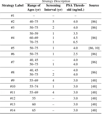
risk groups. The term “onset probability” is synonymous with the term “probability of developing PCa.” . . . 41 Table 3.4 PSA screening strategies compared in this study. Strategy #1 is no screening.
Strate-gies #1–#8 were taken from a prominent simulation study [86]. Strategy #5 was also used in the PLCO trial. Strategies #9–#14 were used in the ERSPC trial.) . . . 43 Table 3.5 Population means and variances of normally-distributed random variables in the
log-PSA growth model expressed in Equation (3.10). The values are taken directly from Gulati et al. [40]. . . 50 Table 3.6 Parameters Used in Our PCa Natural-History Simulation, along with Sources for All
Parameter Estimates. The value of 1.0 as the probability of other-cause death is a modest assumption made in our model only governing transitions at age 100 years. 54 Table 3.7 Lower-bound numerical estimates for parameterwt. The timet(age40Ct) denotes
that the correspondingwt value applies to transitions occurring during the interval
Œt; tC1/. . . 55 Table 3.8 Basecase numerical estimates for parameterwt. The timet (age40Ct) denotes
that the correspondingwt value applies to transitions occurring during the interval
Œt; tC1/. . . 56 Table 3.9 Upper-bound numerical estimates for parameterwt. The timet(age40Ct) denotes
that the correspondingwt value applies to transitions occurring during the interval
Œt; tC1/. . . 57 Table 3.10 Comparing model-estimated PCa mortality and diagnosis rates, lifespan, and
metasta-sized PCa survival time to corresponding estimates from the literature. Whites means white US males with no family history of PCa and CCI=0, AA means African Amer-ican males with no family history of PCa and CCI=0, and mPCa means metastasized PCa. Model estimates obtained by simulating 50,000 patients screened annually from ages 50 to 75 at PSA threshold 4.0 ng/mL, and 95% confidence-interval half widths are given for model estimates. . . 59 Table 3.11 Description of patient and screening characteristics used to simulate each of the 7
major study centers in the ERSPC trial. These quantities are taken from Schr¨oder et al. [95]. . . 60 Table 3.12 Estimates of the expected NNS for screening in each of the compared risk groups
using the screening strategies #1–#14; 95% confidence interval (CI) half-widths are shown in parentheses. Recall that strategy #1 is no screening. . . 69 Table 3.13 Estimates of Clinical Statistics from Screening with Strategy #6 in Each of The
Table 3.14 Clinical statistics for the whites risk group based on samples of 100,000 simu-lated patients under the corresponding screening strategies. CI HW means the 95% confidence-interval half width. Recall that strategy #1 is no screening. . . 71 Table 3.15 Clinical statistics for the African Americans risk group based on samples of 100,000
simulated patients under the corresponding screening strategies. CI HW means the 95% confidence-interval half width. Recall that strategy #1 is no screening. . . 72 Table 3.16 Clinical statistics for the Family History risk group based on samples of 100,000
simulated patients under the corresponding screening strategies. CI HW means the 95% confidence-interval half width. Recall that strategy #1 is no screening. . . 73 Table 3.17 Clinical statistics for the CCI=1 risk group based on samples of 100,000
simu-lated patients under the corresponding screening strategies. CI HW means the 95% confidence-interval half width. Recall that strategy #1 is no screening. . . 74 Table 3.18 Clinical statistics for the CCI2 risk group based on samples of 100,000
simu-lated patients under the corresponding screening strategies. CI HW means the 95% confidence-interval half width. Recall that strategy #1 is no screening. . . 75 Table 3.19 NNS estimates from sensitivity analysis over the annual probability of other-cause
death (dt). For each risk group, the headings “low” and “high” respectively denote the low and high levels of parameterdt. The 95% CI estimates are based on simulated samples of 1 million patients. . . 77 Table 3.20 NNS estimates from sensitivity analysis over the annual probability of developing
PCa (wt). For each risk group, the headings “low” and “high” respectively denote the low and high levels of parameterwt. The 95% CI estimates are based on simulated samples of 1 million patients. . . 78 Table 3.21 NNS estimates from sensitivity analysis over the annual metastasis probability
for patients in state C (et). For each risk group, the headings “low” and “high” respectively denote the low and high levels of parameteret. The 95% CI estimates are based on simulated samples of 1 million patients. . . 79 Table 3.22 NNS estimates from sensitivity analysis over the PCa-screening leadtime (tLT). For
each risk group, the headings “low” and “high” respectively denote the low and high levels of parametertLT. The 95% CI estimates are based on simulated samples of 1
million patients. . . 80 Table 4.1 QALY disutilities in the PCa screening simulation model. . . 108 Table 4.2 Decision-variable (xt) value to PSA-screening threshold rule mappings. . . 117 Table 4.3 Basecase numerical estimates for QALY disutilities in the natural history model. . 154 Table 4.4 Comparison of the screening strategies from Chapter 3 with the optimized strategy
for the whites risk group,xyW, based on estimated expected QG. Estimates are shown with 95% CIs and based on populations (samples) of107independently simulated patients. . . 157 Table 4.5 Comparison of the screening strategies from Chapter 3 with the optimized strategy for
Table 4.6 Comparison of the screening strategies from Chapter 3 with the optimized strategy for the family history risk group,yxFH, based on estimated expected QG. Estimates are shown with 95% CIs and based on populations (samples) of107independently simulated patients. . . 158 Table 4.7 Comparison of the screening strategies from Chapter 3 with the optimized strategy
for the CCID1 risk group, yxC1, based on estimated expected QG. Estimates are shown with 95% CIs and based on populations (samples) of 107 independently simulated patients. . . 159 Table 4.8 Comparison of the screening strategies from Chapter 3 with the optimized strategy
for the CCI2 risk group,yxC2, based on estimated expected QG. Estimates are shown with 95% CIs and based on populations (samples) of 107 independently simulated patients. . . 159 Table 4.9 Definitions of parameters for transition probability matrices. . . 170 Table 4.10 Numerical estimates used as the low and high levels for QALY disutilities in the
sensitivity analysis. . . 171 Table 4.11 Expected QG estimates from one-way sensitivity analysis over model
parame-ters for the White risk group. The symbolD? denotes that all QALY disutilities (DScr;DDia;DBiop;DTre; andDMet) were simultaneously varied to their lowest or
highest plausible levels. . . 171 Table 4.12 Expected QG estimates from one-way sensitivity analysis over model parameters for
the African Americans risk group. The symbolD?denotes that all QALY disutilities (DScr;DDia;DBiop;DTre; andDMet) were simultaneously varied to their lowest or
highest plausible levels. . . 172 Table 4.13 Expected QG estimates from one-way sensitivity analysis over model parameters
for the Family History risk group. The symbolD?denotes that all QALY disutilities (DScr;DDia;DBiop;DTre; andDMet) were simultaneously varied to their lowest or
highest plausible levels. . . 172 Table 4.14 Expected QG estimates from one-way sensitivity analysis over model
parame-ters for the CCID1 risk group. The symbolD?denotes that all QALY disutilities (DScr;DDia;DBiop;DTre; andDMet) were simultaneously varied to their lowest or
highest plausible levels. . . 172 Table 4.15 Expected QG estimates from one-way sensitivity analysis over model
parame-ters for the CCI2 risk group. The symbolD?denotes that all QALY disutilities (DScr;DDia;DBiop;DTre; andDMet) were simultaneously varied to their lowest or
highest plausible levels. . . 173 Table 5.1 Samples of optimized strategies produced by the binary-encoding–scheme method
Table 5.2 Sample statistics on the optimized strategies produced by the binary-encoding– scheme method for each of the compared risk groups using the basecase parameter estimates. The CIs are estimated using the Student-t distribution. PSA thresholds have units ng/mL, and ages and screening frequency have units years. The screening frequency means the time between screen events. . . 202 Table 5.3 Means-based strategies constructed on the basis of the sample means from Table 5.2
of the following quantities: the age to start screening; the age to stop screening; the average PSA threshold, and the frequency of screening. . . 202 Table 5.4 Expected QG estimates across risk groups using basecase parameter levels comparing
strategies #1–#14 from Chapter 3 to the best strategies found by optimization in Chapters 4 (the strategies in Figures 4.15a through 4.15e), and the representative strategies from Chapter 5 (the strategies in Table 5.3). Each estimate is based on a sample of107 simulated patients from the corresponding risk group under the corresponding screening strategy. For each risk group, the labels “opt4” and “opt5” denote, respectively, the corresponding optimized strategy from Chapter 4 and representative strategy from Chapter 5. . . 204 Table 5.5 Expected QG estimates from one-way sensitivity analysis over model parameters
for the Whites risk group, based on samples of 5 independent runs of the GA for each risk-group–experimental-configuration combination. Each estimate is based on a sample of107simulated patients from the corresponding risk group under the corresponding screening strategy. The symbolD?denotes that all QALY disutilities (DScr;DDia;DBiop;DTre;andDMet) were simultaneously varied to their greatest or
smallest plausible values. Seed means the random number seed used in the construc-tion of the initial populaconstruc-tion for the GA and in the crossover and mutaconstruc-tion operators of the GA. . . 208 Table 5.6 Expected QG estimates from one-way sensitivity analysis over model parameters
for the African Americans risk group, based on samples of 5 independent runs of the GA for each risk-group–experimental-configuration combination. Each estimate is based on a sample of107simulated patients from the corresponding risk group under the corresponding screening strategy. The symbolD?denotes that all QALY disutilities (DScr;DDia;DBiop;DTre;andDMet) were simultaneously varied to their
greatest or smallest plausible values. Seed means the random number seed used in the construction of the initial population for the GA and in the crossover and mutation operators of the GA. . . 209 Table 5.7 Expected QG estimates from one-way sensitivity analysis over model parameters
for the Family History risk group, based on samples of 5 independent runs of the GA for each risk-group–experimental-configuration combination. Each estimate is based on a sample of107simulated patients from the corresponding risk group under the corresponding screening strategy. The symbolD?denotes that all QALY disutilities (DScr;DDia;DBiop;DTre;andDMet) were simultaneously varied to their
Table 5.8 Expected QG estimates from one-way sensitivity analysis over model parameters for the CCID1 risk group, based on samples of 5 independent runs of the GA for each risk-group–experimental-configuration combination. Each estimate is based on a sample of107simulated patients from the corresponding risk group under the corresponding screening strategy. The symbolD?denotes that all QALY disutilities (DScr;DDia;DBiop;DTre;andDMet) were simultaneously varied to their greatest or
smallest plausible values. Seed means the random number seed used in the construc-tion of the initial populaconstruc-tion for the GA and in the crossover and mutaconstruc-tion operators of the GA. . . 211 Table 5.9 Expected QG estimates from one-way sensitivity analysis over model parameters
for the CCI2 risk group, based on samples of 5 independent runs of the GA for each risk-group–experimental-configuration combination. Each estimate is based on a sample of107simulated patients from the corresponding risk group under the corresponding screening strategy. The symbolD?denotes that all QALY disutilities (DScr;DDia;DBiop;DTre;andDMet) were simultaneously varied to their greatest or
smallest plausible values. Seed means the random number seed used in the construc-tion of the initial populaconstruc-tion for the GA and in the crossover and mutaconstruc-tion operators of the GA. . . 212 Table 5.10 Samples of optimized strategies produced by the binary-encoding method for the
reference risk group at preclinical dwelling time (tPD) levels of 0, 4, 8, and 12 years.
LIST OF FIGURES
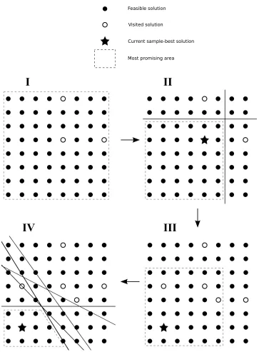
Figure 2.1 Illustrating how solutions are sampled and the most promising area is defined in our COMPASS implementation. . . 18 Figure 3.1 Health states and progression paths in the simulation model. Transitions between
states are represented by arrows. . . 27 Figure 3.2 Sequence of two decision-making stages that take place during each period in the
simulation. . . 29 Figure 3.3 Illustration of the leadtime clock corresponding to a hypothetical patient with PCa
onset at age 42 and with the PSA levels shown from age 40 to 61. . . 48 Figure 3.4 Illustration depicting the divergence between patient histories in the screening and
no-screening simulations. The hypothetical patient depicted in this illustration is shown simulated over 7 periods (years). . . 52 Figure 3.5 Lower-bound, base-case, and upper-bound numerical estimates of parameterwt
inferred from Figure 2 of Haas et al. [44]. . . 55 Figure 3.6 Number of patients simulated for each ERSPC study center. These values are equal
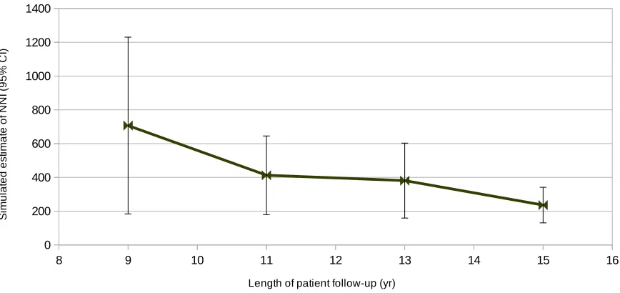
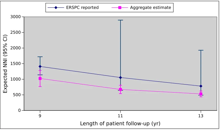
to the minimums of the sizes of the screen and control groups reported for each center. 60 Figure 3.7 Simulation estimates of NNI in each ERSPC trial study center. . . 62 Figure 3.8 Simulation estimates of NNI in the Netherlands study center of the ERSPC trial. . 63 Figure 3.9 Simulation estimates of NNI in the Belgium study center of the ERSPC trial. . . . 63 Figure 3.10 Simulation estimates of NNI in the Sweden study center of the ERSPC trial. . . . 64 Figure 3.11 Simulation estimates of NNI in the Finland study center of the ERSPC trial. . . . 64 Figure 3.12 Simulation estimates of NNI in the Italy study center of the ERSPC trial. . . 65 Figure 3.13 Simulation estimates of NNI in the Spain study center of the ERSPC trial. . . 65 Figure 3.14 Simulation estimates of NNI in the Switzerland study center of the ERSPC trial. . 66 Figure 3.15 Comparison of the aggregated NNI estimates with the NNI values reported by the
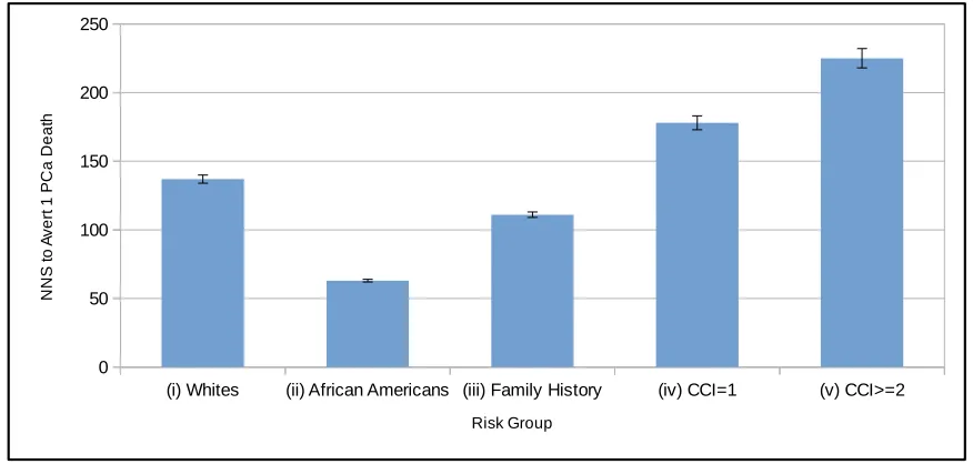
ERSPC trial. . . 67 Figure 3.16 The Estimated NNS to Avert 1 PCa Death for Each Risk Group (i)–(v). Also
displayed are 95% CIs for expected NNS in each risk group based on a sample of 1 million patients. The NNS estimates and associated 95% CIs for risk groups (i)–(v) were, respectively as follows: 137 [134, 140]; 63 [62, 64]; 111 [109, 113]; 178 [173, 183]; 225 [218, 232]. . . 68 Figure 4.1 Sequence of events in the simulation model in a given time period. PSA testing,
prostate biopsy, and definitive PCa treatment take place at the beginning of the period.110 Figure 4.2 Illustration of a PSA threshold vector v containing exactly 2 elements, which
necessarily exhibits an essentially perfectly smooth PSA threshold pattern. . . 121 Figure 4.3 Illustration of a PSA threshold vectorvexhibiting an essentially perfectlyunsmooth
Figure 4.4 Flowchart of three-stage simulation-optimization method. First, the GA broadly explores the feasible region to find a strategy with large expected QG. Then, the clean-up procedure systematically evaluates the strategy from the GA and discards practically insignificant PSA thresholds. Finally, the COMPASS method tries to make regularizing (smoothing) improvements to the cleaned-up strategy without a substantial loss of expected QG. . . 126 Figure 4.5 High-level flowchart of the GA. Beginning with a population (set) of initial
screen-ing strategies, the GA simulates (evaluates) the population. Then, until some prede-termined stopping criterion is met, the GA repeatedly constructs a new population by application of the selection, crossover, and mutation operators, and then simu-lates the new population. . . 127 Figure 4.6 Function call-graph diagram illustrating the organization of algorithms for which
pseudocode is provided. The blue boxes beside the abstract functions RECOMBINE, SELECTION, and CROSSOVERlist the corresponding concrete functions to which the abstract functions may refer. . . 129 Figure 4.7 Illustration of the selection, crossover, and mutation operators in the GA. To
con-struct a single new screening strategy, the GA selects two existing strategies which are then transformed by application of the crossover operator into a single strategy, which is further modified by application of the mutation operator. . . 134 Figure 4.8 Screening strategy with practically-insignificant residual DNA from the GA. . . . 140 Figure 4.9 QALYs-gained observations (i.e.,Dj values) for all screen-detected patients who
benefited from screening under the strategy depicted in Figure 4.8. . . 141 Figure 4.10 Screening strategy from Figure 4.8 after having the practically-insignificant
thresh-olds removed by the clean-up procedure. . . 144 Figure 4.11 Comparison of the 3 recombination strategies for the GA on the ACKL test problem.150 Figure 4.12 Comparison of the 3 recombination strategies for the GA on the BELA test problem.151 Figure 4.13 Comparison of the 3 recombination strategies for the GA on the SALO test problem.152 Figure 4.14 Comparison of the 3 recombination strategies for the GA on the GRWK test problem.153 Figure 4.15 Optimized strategiesxyW;xyAA;yxFH;yxC1;andyxC2produced by the three-stage method
for the White, African American, Family History, CCID1, and CCI2 risk groups, respectively, using the basecase parameter estimates. . . 156 Figure 4.16 Estimated expected QG for each of the compared risk groups for all the
strate-gies from Chapter 3 as well as the stratestrate-gies produced by the three-stage method with basecase parameter values. For each risk group, the label “opt” denotes the corresponding optimized strategy from Figures 4.15a through 4.15e. . . 160 Figure 4.17 Comparison of the estimated expected NNSQ for the basecase optimized strategies
depicted in Figures 4.15a through 4.15e based on samples of107simulated patients from the corresponding risk groups. The 95% CIs reflect inter-patient stochastic variability; they do not reflect generalized uncertainty in any of the model parameters.161 Figure 4.18 Comparison of the estimated expected NNS for the basecase optimized strategies
Figure 4.19 Plots of the # ./y function showing the effect of variation in the certain model parameters on the single-period expected reward for screening 53-year-old men from the reference risk group (the White risk group) at different PSA thresholds ( D0:0; 0:5; : : : ; 10:0ng/mL). . . 164 Figure 4.20 Plots of the # ./y function showing the effect of variation in the certain model
parameters on the single-period expected reward for screening 69-year-old men from the reference risk group (the White risk group) at different PSA thresholds ( D0:0; 0:5; : : : ; 10:0ng/mL). . . 167 Figure 4.21 Optimized strategies produced by the three-stage method for the White, African
American, Family History, CCID1, and CCI2 risk groups, respectively, where no patient is permitted more than 1 prostate biopsy. . . 169 Figure 4.22 Optimized strategies produced by the three-stage method for the White risk group
at different experiments in the sensitivity analysis. The symbolD?denotes that all QALY disutilities (DScr;DDia;DBiop;DTre;andDMet) were simultaneously varied
to their lowest or highest plausible levels. . . 174 Figure 4.23 Optimized strategies produced by the three-stage method for the African
Ameri-can risk group at different experiments in the sensitivity analysis. The symbolD? denotes that all QALY disutilities (DScr;DDia;DBiop;DTre;andDMet) were
simulta-neously varied to their lowest or highest plausible levels. . . 175 Figure 4.24 Optimized strategies produced by the three-stage method for the Family History risk
group at different experiments in the sensitivity analysis. The symbolD?denotes that all QALY disutilities (DScr;DDia;DBiop;DTre;andDMet) were simultaneously
varied to their lowest or highest plausible levels. . . 176 Figure 4.25 Optimized strategies produced by the three-stage method for the CCID1 risk group
at different experiments in the sensitivity analysis. The symbolD?denotes that all QALY disutilities (DScr;DDia;DBiop;DTre;andDMet) were simultaneously varied
to their lowest or highest plausible levels. . . 177 Figure 4.26 Optimized strategies produced by the three-stage method for the CCI2 risk group
at different experiments in the sensitivity analysis. The symbolD?denotes that all QALY disutilities (DScr;DDia;DBiop;DTre;andDMet) were simultaneously varied
to their lowest or highest plausible levels. . . 178 Figure 4.27 Optimized strategies produced by the three-stage method for the reference risk
group at different levels of the preclinical dwelling time (tPD) parameter. . . 180
Figure 5.1 PSA-threshold–based screening strategy decoded fromz1. . . 194 Figure 5.2 PSA-threshold–based screening strategy decoded fromz2. . . 195 Figure 5.3 Estimated expected QG for each of the compared risk groups for all the strategies
LIST OF ALGORITHMS
Algorithm 1 SIMULATION(m) . . . 53
Algorithm 2 SIMULATIONQALYS(m) . . . 114
Algorithm 3 PERIODQALYS(screen, biopsy, age, ageAtTreatment, state, lastState) . . . . 115
Algorithm 4 GENETICALGORITHM(X) . . . 128
Algorithm 5 RECOMBINE STANDARD(X, GENERATION) . . . 131
Algorithm 6 RECOMBINE DETERMINISTICCROWDING(X, GENERATION) . . . 132
Algorithm 7 RECOMBINE MERITOCRACY(X, GENERATION) . . . 133
Algorithm 8 SELECT ROULETTEWHEEL(X) . . . 135
Algorithm 9 SELECT TOURNAMENT(X) . . . 136
Algorithm 10 SELECT UNIFORM(X) . . . 136
Algorithm 11 CROSSOVER ONEPOINT(PARENT1, PARENT2) . . . 137
Algorithm 12 CROSSOVER TWOPOINT(PARENT1, PARENT2) . . . 138
Algorithm 13 CROSSOVER UNIFORM(PARENT1, PARENT2) . . . 138
Algorithm 14 MUTATE(STRATEGY) . . . 139
Algorithm 15 CLEANUP.x/ . . . 143
Algorithm 16 COMPASS(INITIALSTRATEGY) . . . 146
Algorithm 17 DECODESCHEME(BITS) . . . 192
Algorithm 18 GENETICALGORITHM2(X) . . . 198
Chapter
1
Introduction
In 2015 it is estimated that 220,800 new cases of prostate cancer (PCa) will be diagnosed and 27,540 deaths from PCa will occur in the United States [5]. Over the period from 2007 to 2011, African Americans were estimated to be 1.7 times as likely as white US males to be diagnosed with PCa, and 2.4 times as likely to die from PCa [5]. By these estimates, PCa is one of the most common types of cancer affecting US males, and one in which there are ethnic disparities. But screening for PCa is controversial. Some authorities do not recommend routine screening for PCa [78], while many who do recommend screening disagree on how best to screen [98, 16, 15]. Screening for PCa is controversial for two primary reasons: (i) tests to detect PCa are imperfect, and (ii) many researchers and clinicians are apprehensive of the possible harms incurred from overtreatment.
inserting large needles into the prostate gland — for more definitive determination of whether the patient has PCa.
Once PCa is identified by a positive prostate biopsy, the patient and physician may elect to treat the cancer. The early detection and treatment of prostate cancer can add decades to a patient’s life. However, because PCa is a very slow-growing disease, patients with prostate cancer often die of other causes before the cancer metastasizes. Thus, not all PCa treatments result in a gain in life expectancy for the patient. All treatments for PCa do, however, have a high probability of significant side effects from treatment, such as urinary and sexual dysfunction, and in rare cases severe infection and possibly death. Consequently, unnecessary treatment of PCa (referred to as overtreatment) can substantially degrade the quality of a patient’s life.
The use of QALYs is a common way of expressing the overall quality of a particular year of life as a number from 0 to 1. The value of 0 QALYs on one extreme represents death (i.e., no benefit of living whatsoever), and the value of 1 QALY on the other extreme represents a year of perfect health. Values between 0 and 1 represent a less-than-perfect year of life with respect to a patient’s subjective appraisal. By assigning decrements in units of QALYs to certain clinical interventions and undesirable health states, one can make model comparisons not solely on the basis of mortality but also on the basis of different non-fatal degradations to quality of life that can result from diagnosis or treatment of PCa.
There is controversy surrounding PCa screening and the potential impact of screening decisions on many people’s lives due to the potential for overtreatment of men with low-risk and likely indolent PCa. This controversy was caused, in part, by conflicting results from two large randomized trials that studied PSA screening [10, 95]. Much research has been devoted to studying how best to use PSA in screening for PCa. Yet, the question remains hotly debated due to problems with randomized trials including contamination of the nonscreened arms by men who were in fact screened [51, 66]. Moreover, these trial results had limited follow-up and do not account for quality-of-life effects for screened patients.
screening strategies in terms of QALYs.
We conduct extensive sensitivity analysis (SA) of the results from optimization to uncertainties in certain key parameter estimates. We vary parameter estimates in two main ways. First, we selectively vary certain combinations of parameters in order to represent specific known risk groups. Second, in each of these risk groups, we systematically conduct one-way SA on a number of influential model parameters. This SA helps establish robustness in the inferences and conclusions we draw from this research.
After examining the results from two substantially different GA-based simulation optimization approaches, we found strong evidence that PSA was influenced by several physiological factors unrelated to PCa and was therefore not a reliable tool either for diagnosing PCa or for indicating the need to perform a biopsy. In fact, rather than using PSA to selectively biopsy a subset of men at some prescribed age, we found evidence that expected QALYs was maximized whenallmen undergo prostate biopsy (at an age that varies according to risk group). We also found that patients with comorbidities should undergo biopsy earlier in life than patients without comorbidities. These findings were also confirmed using the analytical model based on a formulation of a simplified PCa screening problem in which screening occurs only once for each patient at some defined age. Using simulation to estimate some of the terms in the solution to this analytical model, we found independent support for the conclusions drawn from the simulation optimization methods that virtually all men should undergo prostate biopsy.
carried out, we claim that this inference is very unlikely to be an artifact of inaccurate estimation of model parameters.
This dissertation is structured as follows. In Chapter 2 we present a review of the literature on PCa modeling, screening guidelines, and simulation optimization. We discuss recent guidelines on prostate cancer screening issued by authoritative medical organizations and governmental bodies, prominent randomized control trials and empirical studies to evaluate the impact of PSA screening on prostate cancer mortality, and probabilistic models developed to study the merit of various prostate cancer screening strategies on mortality and quality-of-life. Next, we discuss local and global simulation-optimization approaches. Finally, we discuss the ways in which this dissertation contributes to the body of science on prostate cancer screening and simulation optimization.
In Chapter 3 we evaluate previously recommended PSA screening strategies for different risk groups based on NNS, the expected number needed to screen to avert 1 PCa death. A simulation model of the natural history of prostate cancer is used to evaluate PSA screening in the following risk groups: (i) white US males without a family history of prostate cancer and without comorbidities; (ii) African American males without a family history of prostate cancer and without comorbidities; (iii) white US males with a family history of prostate cancer; (iv) white US males with a Charlson Comorbidity Index (CCI) equal to 1; and (v) white US males with a CCI greater than or equal to 2. This modeling study is designed to answer the following questions:
(a) Which risk groups stand to benefit the least/most from screening in terms of PCa-mortality reduction?
(b) Considering a representative sample of different screening strategies from the literature, which strategy is most efficient for each risk group in reducing PCa mortality?
of 2.5 ng/mL. Therefore, our results suggest that if the sole consideration is reduction of PCa mortality, then a single “one-size-fits-all” strategy may be appropriate for a range of different risk groups.
In Chapter 4, we develop a QALYs-based parameterization of the simulation model from Chapter 3 and use a three-stage simulation-optimization approach to produce clinically realistic improved strategies when PCa mortality is considered along with the quality-of-life degradations stemming from screening and clinical intervention. We also formulate an analytical representation of a simplified single-period PCa screening problem that determines the optimal single-period threshold for screening in terms of maximizing estimated expected QALYs. This model, though much simpler than the real screening problem, is used for supplementary analysis. Following the formulation of this model, we derive point and confidence interval (CI) estimators for the expected reward in QALYs of single-period screening at a given threshold. As an analogue to NNS, we develop and derive a CI estimator for the statistic NNSQ, which is defined as the expected number of patients needed to be screened to produce a net gain in the screened population of 1 QALY. This statistic allows us to utilize variance reduction techniques to improve the efficiency of the simulation optimization method. This three-stage, QALYs-based, simulation-optimization approach is designed to answer the following questions:
(a) When QALYs are considered, which risk groups stand to benefit the least/most from PCa screening?
(b) When QALYs are considered, what is the best way to screen for PCa in each risk group?
Using this approach, we found that there were significant differences in the potential QALYs benefits for different risk groups, with the African American risk group standing to gain the most potential benefit and the comorbidity risk groups standing to gain the least potential benefit. We found the best strategy for each risk group, though not exactly the same across risk groups, was in each case a strategy calling for a biopsy of all men at a particular age (or ages). The most discernible difference between the best strategies for the different risk groups was that biopsy should take place earlier in life for patients with moderate to severe comorbidities (CCI2).
screening strategies without the need for an additional regularizing stage. This alternative approach is designed to answer primarily the same questions we sought to answer in Chapter 4. We use this approach to answer those same questions for the following main reasons: (i) future research on PCa screening may benefit from more than one approach for dealing with the tendency of random-search–based simulation-optimization methods to produce good screening strategies that nevertheless have clinically unrealistic features; and (ii) comparing the results from a second simulation-optimization approach confirms the robustness of our findings with respect to the optimization methodology. This is important due to the likely nonconvex nature of the optimization models. Using this second approach, we obtained results largely concurring with the results from Chapter 4. We also found this approach to be more efficient than the three-stage approach of Chapter 4.
Chapter
2
Literature Review
2.1
Prostate Cancer Screening
In reviewing the literature on PCa screening, we compare and contrast contemporary screening guidelines in Section 2.1.1. We then discuss methods and results from various randomized clinical trials on PCa screening in Section 2.1.2. Finally, in Section 2.1.3, we review PCa screening studies based on probability models.
2.1.1 Guidelines
Some groups, such as the US Preventive Services Task Force (USPSTF) and the American College of Preventive Medicine, recommend against routine PSA-based screening for prostate cancer, basing their recommendation on finding evidence suggesting that screening does not significantly reduce prostate cancer mortality in the general population [70, 78]. Other groups recommend screening in some situations. For example, the American Urological Association (AUA) recommends shared decision-making for men age 55 to 69 years, but does not recommend routine PSA-based screening at other ages [16]. The European Association of Urology (EAU) makes the following statement [47]:
The National Comprehensive Cancer Network (NCCN) provides an algorithm for recommended PSA screening [15] based on discussing risk factors and the possibility of a baseline PSA test. The recom-mended screening frequencies and PSA thresholds for biopsy are different for the age groups 45–75, and
>75 years. And the recommendations stress that men over age 75 should be PSA-tested with caution, especially if they have comorbidities. The American Cancer Society (ACS) recommends that men with at least a 10-year life expectancy be presented around age 50 years with information to make a shared decision whether to undergo screening [98]. They recommend that this discussion begin as early as age 40 or 45 for men at elevated risk for PCa (such as African Americans or men with a positive family history of PCa).
The ACS recommends that the historical 4.0 ng/mL cutoff point still be used, but also that patients with PSA between 2.5 ng/mL and 4.0 ng/mL consider an individualized risk assessment for PCa, particularly for high-grade cancer. It is especially noteworthy that on p. 95 of the 2013 ACSGuidelines on Cancer Screening[98], the following statement appears:
Prostate cancer screening should not occur without an informed decision-making process.
Therefore like the USPSTF, the ACS recommends againstroutinePSA-based screening for PCa without an informed decision-making process.
Finally, the American College of Physicians (ACP) [81] makes the following recommendations about screening for PCa:
Guidance Statement 1: ACP recommends that clinicians inform men between the age of 50 and 69 years about the limited benefits and substantial harms of screening for prostate cancer. ACP recommends that clinicians base the decision to screen for prostate cancer using the prostate-specific antigen test on the risk for prostate cancer, a discussion of the benefits and harms of screening, the patient’s general health and life expectancy, and patient preferences.ACP recommends that clinicians should not screen for prostate cancer using the prostate-specific antigen test in patients who do not express a clear preference for screening.
Guidance Statement 2: ACP recommends that clinicians should not screen for prostate cancer using the prostate-specific antigen test in average-risk men under the age of 50 years, men over the age of 69 years, or men with a life expectancy of less than 10 to 15 years.
Thus we see that like the USPSTF and the ACS, the ACP recommends against routine PSA-based screening for PCa without informed decision making.
European countries also differ in their recommended PSA screening policies. Based on the ERSPC, most European countries (that participated in the study) use the threshold of 3.0 ng/mL, although, Finland, Italy, Holland, and Belgium use the threshold of 4.0 ng/mL [10, 95]. Most European countries use 4-year screening intervals, although Sweden uses 2-year intervals.
2.1.2 Randomized Control Trials
There have been several RCTs to study prostate cancer screening [67, 64, 88, 10, 95, 59]. The two largest of these are the Prostate, Lung, Colorectal and Ovarian (PLCO) Cancer Screening Trial and the ERSPC, the former taking place in the United States. The ERSPC trial found that the rate of death from prostate cancer decreased by 20% as a result of screening, but the PLCO trial found that screening did not achieve a significant mortality reduction [10, 95]. The ERSPC generally used a PSA threshold of 3.0 ng/mL, whereas the PLCO generally used a threshold of 4.0 ng/mL. Thus, the difference in the observed outcomes may be partly due to differences in the screening strategies being evaluated, not to mention differences in prostate cancer incidence and mortality rates between the underlying American and European populations.
the main criticisms was that among participants in the screen arm, those who were prescreened prior to randomization exhibited on average 25% lower prostate cancer mortality than those who were not prescreened. Furthermore, a substantial portion of participants assigned to the control arm actually continued to undergo screening, and subsequent studies have noted that this contamination is likely to weaken the perceived benefit of screening in the PLCO trial [42, 80].
The outcomes of the ERSPC and PLCO trials suggest it may not be possible to accurately evaluate prostate cancer screening strategies using RCTs. This motivates the importance of using quantitative models to investigate the effects of prostate cancer screening on a population.
2.1.3 Prostate Cancer Screening Models
Etzioni et al. [30] formulated an approach for estimating the duration of preclinical prostate cancer, which is prostate cancer that neither has been diagnosed nor has presented symptoms. They derived expressions for estimating the age-specific preclinical incidence rate and prevalence. They then formed the sum weighted by the fraction of a population in each consecutive 1-year age interval from age 30 to 90 of the following quantities: (i) the age-specific preclinical incidence rates; and (ii) the age-specific preclinical prevalences. Finally, they estimated the average preclinical duration as the ratio of the weighted sum of incidence rates to the weighted sum of prevalences. Using data from a Connecticut Surveillance, Epidemiology, and End Results (SEER) registry, US census data, and data from US life tables, they found that the average time spent with preclinical prostate cancer is 11 to 12 years for white males and 10 to 11 years for black males.
predicted the number of prostate cancer deaths prevented, the number of person-years of life saved, the number of PSA tests, and the number prostate biopsies. They presented the relative trade-offs between the benefits and resource implications for each strategy, and found that screening at age 40 and 45 and then screening biennially from age 50 reduced prostate cancer mortality, as well as the number of PSA tests and biopsies when compared with the standard US strategy of annual screening from age 50.
A group of researchers from the Cancer Intervention and Surveillance Modeling Network of the National Cancer Institute, theProstate Working Group, have studied, developed, and compared models of the natural progression of prostate cancer for over 10 years.1Using results from the Rotterdam section of the ERSPC, Draisma et al. [25] modeled the development of prostate cancer up to the point of diagnosis as a Markov process with 9 states defined by all combinations of 3 different cancer stages and 3 different cancer grades. Screening for prostate cancer in the model consisted of events with sensitivity depending on the stage of an underlying cancer. Three variants of this basic model were considered. The first variant included the simulation of cancer that would be detectable as localized cancer by biopsy but would never have been otherwise diagnosed, since such cancers were suggested by the high detection rates among screened men in the ERSPC data. The second variant sampled the duration of preclinical cancer stages based on different probability distributions in order to produce higher variance in the length of time a patient spends in a given cancer stage. The third variant prevented the tumor grade from changing once it became detectable by screening. Using these model variants, they predicted lead times and rates of overdiagnosis for screening at different intervals, and found that lead times and overdiagnosis rates were more favorable for screening intervals larger than 1 year. They also produced evidence that screening may advance diagnosis by more than 10 years.
Etzioni et al. [31] used a Markov chain–based natural-history model of prostate cancer to examine the optimal frequency for normal-risk males to undergo PSA testing. Using rates of disease onset and transition rates between stages (defined by the Whitmore-Jewett staging system), the model generates the age of onset of prostate cancer and the duration in each cancer stage for a fixed cohort of US males. For each patient, the model uses reported lifetime probability of clinical presentation to determine randomly whether the patient will ever be clinically diagnosed. An initial PSA value is randomly generated for each
patient, and each subsequent year the patient’s PSA value increases by a percentage (plus a small random error) that depends on the patient’s cancer stage and stage duration. Using their model, they consider 5 different screening strategies on the basis of benefits harms, specifically, the number of life-years saved from screening and the number of false positive PSA tests and rate of overdiagnosis. They found that screening every 2 years was a cost-effective alternative to the standard US strategy of annual screening. Etzioni et al. [32] used a simulation model to investigate whether population PSA screening could be responsible for the decline in prostate cancer mortality observed from 1992 through 1994. The simulation model identified patients to be PSA-tested and PSA-testing–diagnosed based on a PSA utilization database, recorded PSA testing rates, and linked SEER–Medicare data. Based on a range of estimates for how often PSA screening is used for diagnostic purposes and how often it is used for screening, the model then selected a portion of the PSA-testing–diagnosed patients to have been diagnosed early, i.e., diagnosed at a time when the cancer is amenable to definitive treatment. Using an estimate of the decreased risk of death from prostate cancer by screening, and an estimate of the time by which diagnosis is advanced by screening (lead time), the simulation model generates a date of death for the patient with screening and a date of death for the patient without screening. Using the decreased risk of dying from prostate cancer by screening, they computed the rate of death from prostate cancer prevented by screening. This rate was added to the observed prostate cancer mortality rate to produce a mortality rate reflecting the absence of screening. Using a rate of screening efficacy matching the rate hypothesized for the PLCO trial, they computed an adjusted prostate cancer mortality rate for the period from 1988 to 1994, and found that only very short lead times would result in PSA screening being potentially fully responsible for the observed decline in prostate cancer mortality.
were, respectively, 7 and 5 years, with corresponding overdiagnosis rates 44% and 29%, respectively. After adjusting for the expected lifetime probability of latent undiagnosed prostate cancer during the era before the advent of PSA screening, the overdiagnosis rates for blacks and whites during that era were estimated to be at most 37% and 15%, respectively.
In order to assess whether PSA screening was responsible for the decline in prostate cancer–specific mortality since the 1990s (a research objective similar to that of Etzioni et al. [32]), Etzioni et al. [35] adapted the model from Etzioni et al. [31] to simulate life histories for the US population corresponding to several different birth cohorts between 1980 and 2000. The model generates a set of natural histories and clinical case histories, and then pairs the clinical histories that include diagnosis with natural histories based on birth cohort year, age of disease onset, and age of diagnosis. For clinical histories where no diagnosis occurs, clinical histories are paired with the remaining unmatched natural histories so that age at other-cause death in the clinical history precedes the age of distant-stage incidence in the natural history. For each birth cohort, PSA screening histories are simulated based on reported data on interscreening intervals. Simulated patients with a PSA value greater than 4 ng/mL underwent prostate biopsy with a probability based on data from the PLCO trial. Results from the model suggested that 80% of the decrease in incidence of advanced-stage prostate cancer since 1990 was attributable to prostate cancer screening.
function incorporating a multiplicative trend function to account for changes in the general practice of prostate cancer screening. Third, they modeled PSA screening using a PSA simulator based on linked SEER–Medicare data and results from the National Health Interview Survey. Using PSA screening trends, the model estimates incidence in the presence of PSA screening as well as the distribution of lead times. By 2000, the FHCRC and UMICH models project that PSA screening may explain, respectively, 45% and 70% of the decline in prostate cancer mortality.
Gulati et al. [41] studied the risk of clinical progression and prostate cancer–specific death after detection of prostate cancer in the absence of definitive treatment using 3 models discussed above: the FHCRC [32], MISCAN [25], and UMICH [106] models. For all 3 models, incidence rates were derived from data in 9 SEER registries covering the period from 1975 to 2000. Disease progression levels were defined as Gleason Scores in the ranges 2–7 and 8–10. Other-cause mortality rates were derived from US life tables. And a common Poisson regression model was used to model prostate cancer survival [2]. The models projected that without early detection or definitive treatment, 12%–25% of US males with preclinical onset would have died due to prostate cancer. If left without definitive treatment, prostate cancers diagnosed by positive biopsy with Gleason Score 2–7 and 8–10 would later cause prostate cancer death with probabilities 0.23–0.34 and 0.63–0.83, respectively.
also reducing harms associated with overdiagnosis.
2.2
Simulation Optimization
Simulation optimization is any instance of optimization where the objective function is evaluated by simulating a stochastic system; the simulator is effectively ablack boxthat returns a value often with no clear analytic expression of the function. Stochastic problems which lack properties such as convexity and optimal substructure are not amenable to optimization methods such as stochastic programming or stochastic dynamic programming, but are often amenable to simulation optimization. Fu [38] reviews a host of optimization techniques, including tabu search, simulated annealing, and genetic algorithms, which are suited to optimize problems in which the objective function must be approximated by simulation, and discusses the challenges presented by, and the growing interest in, simulation optimization. Other excellent reviews of simulation optimization are [56] and [102]. Andrad´ottir [8] provides an excellent review of simulation-optimization based on random search methods.
Simulation optimization problems are often solved by implementing a GA, one of the approaches taken in this thesis, such as described in [27] and [24]. GAs are conceptually rooted in the evolutionary laws of natural selection, and are members of the larger class of evolutionary algorithms. Like natural selection, GAs improve a system over time by repeatedly modifying a population of candidate solutions in such a way that better candidate solutions are promoted over time. In 1975, Holland [53] proposed this natural concept as an algorithmic tool for systems modeling and analysis .
GAs have been widely applied across diverse disciplines. Cryptanalysts have used GAs with an initial population comprising guessed keys to attempt to decrypt intercepted cyphertext [75]. Astronomers have used GAs to fit models of the rotation curve of a distant galaxy [18]. Electrical engineers have used GAs to aid in the design of digital signal processing and analysis filters [45]. The common thread that unites these and many other applications, is the use of GAs to overcome the computational intractability of certain problems.
COMPASS can be considered a framework because key components of the framework can be significantly modified without violating several mild assumptions that are sufficient conditions for COMPASS to asymptotically converge to a locally optimal solution.
COMPASS is a sampling-based stochastic-search optimization method. The key feature of COMPASS is the “most-promising area” (MPA), which is defined to be the set of feasible solutions that are at least as close to the current sample-best solution as they are to other visited solutions [55]. Thus, the MPA is fully defined given the set of feasible solutions, the set of solutions that have previously been explored (visited solutions), and the current sample-best solution. At any iteration, COMPASS conducts stochastic search confined to the feasible solutions in the MPA.
An implementation of COMPASS begins with an initial solution (or multiple initial solutions). The expectation of the stochastic objective function is estimated for these solutions (usually by simulation), and the current sample-best is identified by comparing the sample-mean objective-function values of all the solutions. Given the current sample-best solution and the other initial solutions (if there are multiple initial solutions), the MPA is updated. If there is only 1 initial solution, which of course must be the current sample-best solution, then the MPA will be the entire feasible region; otherwise, the MPA will be a subset of the feasible region containing solutions that are at least as close to the current sample-best solution as they are to the other initial solutions.
On subsequent iterations of an implementation of COMPASS, solutions are randomly sampled within the MPA, and all visited solutions — the set of visited solutions includes the sample-best solution and the newly sampled solutions — are evaluated based on some defined simulation-allocation rule (SAR). Then, the current sample-best solution is updated by comparing the sample-mean objective-function values of all visited solutions, which may or may not result in the current sample-best solution changing. Once the sample-best solution is updated, then the MPA is updated, and COMPASS proceeds to the next iteration unless some defined stopping criterion is satisfied.
SAR, it is necessary only to simulate the number ofadditionalreplications (observations) of each solution in order to satisfy the total number of replications required of each solution by the SAR. The accumulation of simulation observations over the iterations of COMPASS reduces the overall computational costs of the method.
Figure 2.1 illustrates four iterations of COMPASS. In Figure 2.1, each of the black dots represents a feasible solution to a hypothetical two-dimensional discrete solution-space. In step I, the MPA (denoted by the dashed border) is the entire set of feasible solutions, and 3 initial solutions (white dots with black borders) are chosen. Because we have sampled or explored these solutions, they are considered visited solutions. In step II, the sample-best (denoted by the star) is selected from the current set of all visited solutions, and the MPA is updated.
The MPA is updated by constructing hyperplanes separating the sample-best solution from the other visited solutions. A hyperplane is constructed between the sample-best solution and each other visited solution. Each hyperplane separates feasible solutions that are at least as close (in Euclidean norm) to the sample-best solution as to the given visited solution from all other feasible solutions that are closer to the given visited solution than to the sample-best solution. In the two-dimensional case, each hyperplane would be the perpendicular bisector of the line segment connecting the sample-best solution to the given non-sample-best visited solution. Note that the MPA can be defined by separating hyperplanes that, together with the implied hyperplanes at the boundaries of the finite feasible region, form a convex polyhedron. In particular, to form the MPA polyhedron, one constructs for each non-sample-best visited solution the hyperplane normal to the line containing that non-sample-best visited solution and the sample-best solution. In the two-dimensional problem in Figure 2.1, the separating hyperplanes are lines perpendicular to lines containing a visited solution and the sample-best solution.
Now, in step III, 3 new solutions are sampled from the updated MPA, and the sample-best solution changes. Finally, in step IV, the MPA is updated based on the entire set of visited solutions and the new sample-best solution discovered in step III.
Feasible solution
Visited solution
Current sample-best solution
Most promising area
I
II
IV
III
grows larger than 10. They proposed a new scheme for sampling solutions from the MPA calledcoordinate sampling; in coordinate sampling, new solutions are sampled by simply shifting the sample-best solution in one coordinate direction instead of sampling solutions uniformly randomly from the MPA. They found that coordinate sampling reduced the computational overhead of COMPASS by as much as 1000 times. Recently, Xu et al. [111] developed an local-search alternative to COMPASS called the adaptive hyperbox algorithm (AHA). There are many similarities between COMPASS and AHA; indeed, AHA was inspired by COMPASS. Unlike COMPASS, however, the MPA in AHA is always defined by a
d-dimensional hyperbox, whered is the number of decision variables. In COMPASS, the MPA is constructed by hyperplanes separating the sample-best solution from each other solution in the visited set. Consequently, when the number of visited solutions grows very large, then construction of the MPA, which occurs at every iteration of COMPASS, can become time-prohibitive. In AHA, the MPA is constructed or modified at each iteration by simple shifting each facet of the hyperbox in one coordinate direction. For problems of many decision variables, AHA is shown to perform as well as COMPASS.
Xu et al. [110] recommend that the optimal computing budget allocation (OCBA) procedure be used as the SAR in COMPASS. Given a set of solutions, OCBA determines the number of simulation replications required for each solutionxi in order to maximize the probability that the solution with highest sample-mean performance is truly the solution with highest expected performance. Letv.xi/
denote the expected performance of solutionxi, letv.xxi/denote the sample-mean estimator ofv.xi/
obtained by m0i independent replications of the simulation at solution xi, let i2 denote the sample variance of them0isimulation-generated responses at the solutionxi, letbdenote the index of the solution with highest sample-mean performance, and letkdenote the number of solutions being compared. Then the probability of correct selection for a maximization problem in which we take solutionxbto be the best solution is defined as
From Chen [21] we know that a lower bound onPfCSgcan be computed by
PfCSgLB D
k
Y
iD1;i¤b
Prfxv.xb/ >xv.xi/g: (2.2)
Because Equation (2.2) is a lower bound onPfCSgthat can be quickly computed from the sample-mean performance estimates for solutionsx1; : : : ;xk, OCBA uses this approximation to estimate the probability of correct selection.
OCBA utilizes the concept of signal-to-noise ratio. The “signal” in OCBA for a given solutionxi is the differenceıb;i D xv.xi/ v.x xb/between the sample meanv.xxi/of that solution and the sample mean v.N xb/ of the current sample-best solution. The “noise” in OCBA for a given solution is that solution’s sample variancei2. The fundamental principle of OCBA is to allocate simulation replications to the various solutions in proportion to their signal-to-noise ratios. If a solution has a relatively high signal-to-noise ratio, we know with a high probability that this solution is not actually the best of the solutions under consideration. On the other hand, if a solution has a relatively low signal-to-noise ratio, then we know with a lower probability that this solution is not actually better than the current sample-best solution.
From Chen and Lee [22], we know that given a computing budget ofBsimulation replications, we can maximize the approximate probability of correct selection asymptotically asB ! 1by solving the equations
mi
mj D
i=ıb;i
j=ıb;j
2
; i; j 2 f1; 2; : : : ; kg; andi ¤j ¤b; (2.3)
mb Db
q
k
X
iD1;i¤b
m2i
i2; (2.4)
k
X
iD1
mi DB: (2.5)
chosen by experimentation for a given problem. Every timeBis increased, Equations (2.3), (2.4), and (2.5) are solved and each solutionxi is evaluated by executingmi m0i additional simulation replications. This iterative process allows OCBA to gradually learn more about the true mean and variance of each solution, and, at each iteration after the first, correct poorer mean and variance estimates from the preceding iteration.
2.3
Contributions of this Dissertation
This dissertation contributes to the existing literature in the following ways. First, our research constitutes to the best of our knowledge the first simulation-optimization study of PCa screening across ethnic, hereditary, and comorbidity risk groups. Although randomized clinical trials have studied the effect of prostate cancer screening in different populations, they are costly, time-consuming, and lack the freedom to explore more than a handful of alternative screening strategies. Randomized clinical trials also suffer from contamination and other sources of bias, as described previously in this chapter. Our research, which uses simulation rather than real trial patients, is unencumbered by the financial and ethical constraints that preclude consideration of a vast array of untried and unexplored possible screening strategies. This research can be extended by modeling additional risk groups, such as subgroups within the groups we considered. Additionally, this model could be modified to consider additional non-PSA-based PCa biomarkers.
optimization), it also allows us to model a range of important aspects of the problem that would otherwise be extremely challenging, if not practically infeasible. For example, we model clinical detection of PCa on the individual patient level by monitoring the time that a patient spends with PCa, and we use this time in conjunction with empirical PCa-leadtime estimates to determine when (if ever) a given patient will present symptoms of PCa that lead to clinical detection. To model the same monitoring process in a Markov model would require a large state-space expansion, and the transition probabilities between states in the expanded space might be very difficult to estimate accurately. Another example of the advantage of relaxing the Markov assumption is our use of a widely accepted method for sampling patient PSA levels based on a linear changepoint model of PSA growth [40]. In this method, each patient’s PSA trajectory over time is based on the age at PCa onset (if onset occurs for the given patient) and several randomly-sampled, continuous, patient-specific, PSA-model parameters. Such a PSA model does not have a tractable Markov representation, because each patient’s future PSA trajectory depends not merely on the patient’s present PSA level but also on previous values of the PSA level and on the time of PCa onset (if applicable). These two examples demonstrate the value in using a simulation-optimization approach as opposed to a dynamic-programming approach because both clinical detection and PSA growth over time are important components of the PCa screening problem.
Third, we have carefully validated important aspects of our simulation model such as life expectancy, PCa diagnosis and mortality, and metastasis survival. We validated the novel PCa leadtime–based implementation of clinical detection together with other components of the simulation model by using simulation to reconstruct the ERSPC trial and compare the corresponding simulation NNS estimates with the published reports on the outcomes of the ERSPC.
Fourth, we demonstrate how careful synchronization of simulated patient histories can be used as a variance-reduction technique to evaluate and compare screening strategies on the basis of QALYs. The NNSQ statistic is easily interpreted by a clinical audience because of its conceptual similarity to the widely-used NNS statistic. Therefore, we contend that NNSQ is an excellent performance measure for a comparative simulation study of disease screening or treatment strategies.
in the time series of PSA test thresholds. Because of the tendency of simulation-optimization methods to produce strategies with erratic patterns of PSA test thresholds, and because such irregular strategies would be difficult to implement in practice and easy to misinterpret, these methods may prove valuable to future simulation-optimization research in disease screening and treatment. This research could be extended by investigating additional approaches for inducing regularity in the decision-variable time series. For example, the binary-encoding scheme could be modified for the PCa screening problem by assuming a nonlinear rate of change in the PSA threshold over time.
Chapter
3
Simulation of PSA-Based Prostate Cancer
Screening for Heterogeneous Patient Risk
Groups
3.1
Introduction
recommend screening in the context of a shared decision-making process for some patients that considers individual patient preferences, life expectancy, and risk factors such as race and family history of PCa [16, 98].
Differences in incidence and mortality rates, as well as variation in the predictive value of PSA, can affect the balance of harms and benefits of screening within demographic subpopulations of US males [85, 105]. Estimating the public-health implications of screening in these various subgroups is further complicated by both the large number of proposed screening strategies and the difficulty of estimating common performance measures for screening such as the expected number needed to screen (NNS) to avert 1 PCa death [10, 95].
We developed and used a computer simulation of PCa screening, derived from a stochastic-process model of the natural history of the disease, to compare screening strategies for five demographic groups based on race (white and African American), family history of prostate cancer, and different levels of comorbid medical conditions. Using estimates of the incidence, other-cause mortality, and PCa mortality rates associated with each risk group, we compared published PSA screening strategies to find the strategy that minimized the expected NNS for each subgroup.
3.2
Methodology
A stochastic-process model of the natural history of PCa from Underwood et al. [107] was adapted and combined with a method for sampling patient PSA histories and a method for incorporating clinical incidence of PCa to predict the effects of published screening strategies on different risk groups. We developed a method of synchronizing patient histories between screening and no-screening simulations in order to estimate expected NNS. Different risk groups were modeled by varying relevant model parameters based on ratios reported in the literature.
from a multi-center Scandinavian study instead of a largely regionally-local set of patients under care at Mayo Clinic. The annual probability that untreated PCa metastasizes is now estimated according to length of time since PCa onset (with a metastasis probability of 0 during a specific “preclinical dwelling interval”), whereas in Underwood et al. [107] a single fixed probability was used independent of how long a given patient had PCa. The annual probability of PCa-specific death is based on SEER data both in Underwood et al. [107] and in this research, but the estimates in this research are based on a more-recently published SEER Survival Monograph.
In addition to improved estimates of various model transition probabilities, the model in this research surpasses the model in Underwood et al. [107] by the use of PCa leadtime in the simulation of clinical (nonscreen) detection of PCa. Accounting for clinical incidence of PCa is important because it influences the overall absolute benefit that can be realized by screening.
In the model in this research, we also have a more detailed set of QALY disutilities, and the disutility estimates come from a prominent recent study of quality-of-life and PCa screening. Previously, in Underwood et al. [107], the estimates for the various QALY disutilities were pooled from more than a single source. Furthermore, previously the disutility estimate for biopsy was based on a disutility estimate from another similar biopsy procedure; in this research, we have a much better estimate for the disutility of biopsy, and it is significantly smaller than the previous estimate inferred from a nonprostate biopsy procedure. Finally, in much of this research we permit men to undergo more than 1 prostate biopsy during their lives. Previously, we restricted all patients to at most 1 biopsy.
3.2.1 Patient Health-State Stochastic Process
Screen detection
Death from PCa Disease-free
patient
Patient had metastasized PCa, but died of other causes
PCa onset
Metastasis of untreated PCa
Patient had PCa, but died of other causes
Clinical detection No PCa
PCa (undetected)
Posttreatment
for PCa Metastasis from PCa
PCa specific mortality All-other-cause
mortality