Test Protocols for Evaluating Commercial Microgrid Controller.

(1)

ABSTRACT

LONG, QIAN. Test Protocols for Evaluating Commercial Microgrid Controller. (Under the direction of Dr. David Lubkeman).

(2)

(3)

Test Protocols for Evaluating Commercial Microgrid Controller

by Qian Long

A thesis submitted to the Graduate Faculty of North Carolina State University

in partial fulfillment of the requirements for the degree of

Master of Science

Electrical Engineering

Raleigh, North Carolina 2016

APPROVED BY:

_______________________________ _______________________________

Dr. Srdjan Lukic Dr. Ning Lu

_______________________________ Dr. David Lubkeman

(4)

ii

DEDICATION

To my parents and grandparents for their unconditional love. To my teachers for their precious life lessons.

To all my friends for their care and support.

(5)

iii

BIOGRAPHY

Qian Long was born in Jianli, China. He received his Bachelor of Science degree in Electrical Engineering and Automation from China Agricultural University in June 2014. He started to pursue a Master of Science degree in Electrical Engineering in North Carolina State University in August, 2014. His research interests include distribution system analysis, Volt/VAR control and microgrids.

(6)

iv

ACKNOWLEDGEMENTS

I would first like to express the sincerest gratitude to my advisor, Dr. David Lubkeman, for his continuous patience, guidance and support through the completion of my thesis. I appreciate his giving me the amazing opportunity that allows me to be exposed to the exciting fields of microgrid operation and control. His advice on academics as well as careers are priceless and his constant hard work and commitment inspire me to keep working and studying harder.

I would also like to thank Dr. Ning Lu and Dr. Srdjan Lukic, not only for serving my thesis committee, but also for their insightful comments and suggestions on my research.

My thanks also go to my lab mates, Yuhua, who has been a wonderful teammate and has developed battery and inverter models for the testbed, Xinyang, who has provided resourceful information on DNP3 communication, Xiangqi and Jian, who has designed PV, load and CHP models for the testbed. It would be impossible for me to complete the thesis without their great contribution.

I also sincerely thank my friends Sen Yang, Lei Mao, Shaoliang Nie and Boxuan Zhong for their care and friendship. In particular, I would like to give thanks to Weifeng Li for stimulating me to learn and grow as a graduate student and a researcher.

(7)

v

LIST OF TABLES

Table 2.1 Mapping on feeders to microgrid zones ... 15

Table 2.2 Critical load groups vs noncritical load groups ... 16

Table 2.3 Olney Town Center microgrid resource portfolio ... 16

Table 2.4 Comparison of short circuit values between full and reduced models ... 32

Table 3.1 Table of functional test cases ... 37

Table 3.2 Microgrid efficiency test results ... 40

Table 3.3 Reliability of distribution components ... 41

Table 3.4 Customers distribution information ... 43

Table 3.5 Microgrid reliability test results ... 44

Table 3.6 Baseline performance analysis (no microgrid) ... 44

Table 3.7 Microgrid Greenhouse Gas test results ... 47

Table 3.8 Summary of test variations ... 48

Table 3.9 Test variation coding scheme ... 49

Table 3.10 Energy management - grid connected test procedures ... 51

Table 3.11 Energy management - islanded test procedures ... 53

Table 3.12 Intentional islanding - stability test procedures ... 55

Table 3.13 Unintentional islanding - external test procedures ... 57

Table 3.14 Unintentional islanding - internal test procedures ... 59

(10)

viii

LIST OF FIGURES

Figure 1.1 A typical microgrid schematic [4] ... 2

Figure 1.2 DOE microgrid activities in United States [5] ... 4

Figure 1.3 CERTS microgrid schematic ... 5

Figure 1.4 IIT microgrid system configuration [11] ... 6

Figure 1.5 Resource mix and energy flows in UCSD microgrid [13] ... 7

Figure 1.6 Critical load groups in Olney Town Center [14] ... 9

Figure 2.1 Olney Town Center microgrid zones ... 14

Figure 2.2 Olney distribution systems (orange – feeder 15119, blue – feeder 15125, yellow – feeder 15126, magenta – feeder 15129) ... 14

Figure 2.3 PV system block in Simulink ... 18

Figure 2.4 PV system general structure ... 18

Figure 2.5 Referenced real world PV profile ... 19

Figure 2.6 Simulated PV system output power ... 19

Figure 2.7 Critical load groups block in simulink ... 20

Figure 2.8 Critical load groups general structure ... 20

Figure 2.9 Referenced real world load profile ... 21

Figure 2.10 Measured load group input power ... 21

Figure 2.11 Block diagram of a CHP unit... 22

Figure 2.12 Simulink diagram of a CHP unit ... 23

Figure 2.13 Block diagram of the micro-turbine in a CHP unit... 23

Figure 2.14 CHP electrical output versus power output reference command under grid-connected mode ... 24

Figure 2.15 Speed response between transitions from grid-connected mode to islanded mode ... 25

Figure 2.16 Thermal loads versus thermal energy provided by Chiller ... 25

Figure 2.17 Energy storage system model block diagram ... 25

Figure 2.18 Dual polarization battery model ... 26

Figure 2.19 Schneider inverter model block diagram [20] ... 26

Figure 2.20 IQ-V characteristic of the voltage control function [20] ... 27

Figure 2.21 Olney Town Center microgrid master one-line diagram ... 30

(11)

ix

Figure 2.23 FREEDM microgrid test environment ... 33

Figure 2.24 Communication test validation: (a) CHP dispatch value from 200kW to 240kW (b) BESS charging/discharging rate from 10kW to -10kW ... 34

Figure 2.25 Energy dispatch – long-term simulation ... 35

Figure 3.1 Outage map for feeder 15126 ... 42

Figure 3.2 Microgrid Zone 1 one line diagram for reliability analysis ... 45

Figure 4.1 Test environment diagram ... 62

Figure 4.2 DNP3 master-slave configuration ... 63

Figure 4.3 Test architecture diagram ... 64

Figure 4.4 Example of the configuration file for multiple slave devices ... 64

Figure 4.5 OpWriteFile block ... 67

Figure 4.6 Post-processing workflow ... 67

Figure 4.7 TestDrive signal tree ... 68

Figure 4.8 TestDrive console interface ... 69

Figure 4.9 Testing workflow ... 71

Figure 4.10 LabVIEW test master ... 72

Figure 5.1 Predefined dispatch schedule of CHP and BESS from LabVIEW master ... 74

Figure 5.2 (a) Electricity dispatch (b) Energy production ... 75

Figure 5.3 Evaluation of baseline (no DERs) vs microgrid ... 76

Figure 5.4 CHP fuel efficiency vs temperature ... 77

(12)

x

LIST OF ABBREVIATIONS

BESS Battery Energy Storage System

CERTS Consortium for Electric Reliability Technology Solutions

CHP Combined Heat and Power

DER Distributed Energy Resources

DG Distributed Generation

DNP3 Distributed Network Protocol

DOE U.S. Department of Energy

DR Demand Response

DSM Demand Side Management

ESP Energy Service Provider

GHG Greenhouse Gas

MMC Microgrid Master Controller

PCC Point of Common Coupling

SAIDI System Average Interruption Duration Index

(13)

1

Chapter I. Introduction

1.1 The Microgrid Concept

Distribution grids are experiencing an evolution, often noted as Smart Grid. A smart grid generally refers to an electricity network that employs a class of innovative technology, including intelligent monitoring, control, and communication, in order to offer more reliable, resilient, affordable and sustainable electric services. Increasing integration of renewable energy resources, aging infrastructure of electrical systems, extreme weather events, and system security and resiliency needs. Those are all leading to these significant changes in how electricity is generated, distributed, managed and consumed. The availability of smart grids is critical to social, economic and environmental benefits [1, 2].

Microgrids, also characterized as the “building blocks of smart grids”, are perhaps the most promising, novel network structure [2]. The key feature that distinguishes microgrids from any other type of distribution network structure is its control capabilities over local distribution network operation through DERs, such as energy storage devices, PV arrays, wind turbines, controllable loads and distributed generators. Generally, these control capabilities allow microgrids to be managed in an optimally economical and sustainable manner, interconnected to the main grid. However, due to grid faults or other interruptions, the microgrids can also be transitioned via appropriate control strategies into islanded operation mode, thus enhancing the resiliency of electric services. Since consequences of adverse weather, like hurricanes and ice storms, have driven a desire to make the power system more resilient, the microgrid technology has been drawing more and more attention in recent years [3].

Up to now, there is no agreement on the architecture of microgrids, or on how large or small microgrids should be with respect to energy capacity and geographic area. But there’s one common feature: The microgrid should be able to isolate from the main grid and independently manage generation assets and balance the critical electric loads within the microgrid. The key components that enable this feature are: the circuit breakers that isolate the microgrid at the PCC or multiple PCCs, the microgrid controller that operates the system and maintains system stability and DERs. In the thesis, a definition of a microgrid from U.S. Department of Energy Microgrid Exchange Group is used:

(14)

2

A typical schematic of a microgrid system is shown as Figure 1.1. It is a community area served by one or more distribution substations and also supported by high penetrations of local DERs such as energy storage systems, micro-turbines, fuel cells and DR. Microgrid systems heavily rely on microgrid control center to provide monitoring, communication and control capabilities across the area in order to achieve a more sustainable, reliable, and economical electric energy system operation.

Figure 1.1 A typical microgrid schematic [4]

1.1.1 Overview of Potential Microgrid Impacts [2]

A microgrid can offer a large variety of economic, technical, environmental and social benefits to consumers, microgrid owners and utility:

(15)

3

Technical – The microgrid can improve the technical performance of the distribution grid in the following aspects: 1) Energy efficiency improvement due to network loss reduction and the utilization of CHP units; 2) Control over power quality via demand side management, coordinated reactive power control and constrained active power dispatch,; 3) Transmission congestion reduction; 4) Ancillary services for supporting grid stability; 5) Grid reliability enhancement via microgrid islanded operation when loss of main grid.

Environmental – The generation in the microgrid leads to a shift towards renewable energy and thus a low GHG emission. On the other hand, the utilization of more energy efficient solutions like CHP and DSM is facilitated by control operation of microgrids.

Social – The microgrid application can raise public awareness and foster incentives for saving energy and reducing carbon emission as well as creating new research topics and job opportunities. For remote or rural regions, the microgrid technology provides a promising solution of electrification.

All the impacts listed above are easy to understand in qualitative aspects but will be less easier to study quantitatively. It is not only because the quantification of microgrid benefits itself is abstract and tentative, but also because it is a multi-objective multi-stakeholder problem where the solution requires some degree of coordination.

1.1.2 Real World Microgrid Demonstration

(16)

4

Figure 1.2 DOE microgrid activities in United States [5]

CERTS Microgrid [6, 7, 8]

The CERTS microgrid was initiated in 1999 to respond to a call from U.S. Congress to restart a federal transmission reliability R&D program and it was implemented to address the concerns on grid reliability technology [9]. It was demonstrated at a full-scale test bed built at American Electric Power Walnut site near Columbus, Ohio, sponsored by the California Energy Commission PIER Electric Transmission Research Program Its participants included University of Wisconsin-Madison (PSERC), Sandia National Laboratories, Woodward, Princeton Power Systems, Northern Power Systems, Tecogen, and Lawrence Berkeley National Laboratory.

(17)

5

Figure 1.3 CERTS microgrid schematic

The CERTS Microgrid Demonstration accomplished its objective of enhancing the ease of integrating small energy sources into a microgrid by developing three advanced techniques [7, 10]: 1) a method for effecting automatic and seamless transitions between grid-connected and islanded modes of operation; 2) an approach to electrical protection within the microgrid that doesn’t depend on high fault currents; and 3) a method for microgrid control that achieves voltage and frequency stability under islanded conditions without requiring high-speed communications.

The IIT Perfect Power Systems

DOE and private industry partners sponsored the Perfect Power initiative, launched by the Galvin Electricity Initiative at Illinois Institute of Technology (IIT) in 2008, together.

The construction of the microgrid involves the entire IIT campus, driven by facts that [11]: 1) The occurrence of at least three power outages per year resulted in a series of teaching and research disruptions with an estimated cost of $500,000 annually;

(18)

6

Figure 1.4 IIT microgrid system configuration [11]

Key features of the IIT Perfect Power microgrid include:

1) High Reliability Distribution System (HRDS) is implemented by replacing old radial distribution systems with new redundant looped systems using fully automated switches shown in Figure 1.4. If the disturbance occurs in the loop, it can be isolated by the switches within 6 cycles and the system can still supply power to all the buildings.

2) A three level hierarchical controller, the Intelligent Perfect Power System Controller (IPPSC), is designed to interface, coordinate, and control the actions of building controllers, HRDS controllers and distributed generation controllers inside the campus. Besides, it allows the microgrid to respond to real time pricing of electricity demand through communication outside with ISO and utility. This system coordinates how much electricity is needed and what load services can be deferred or curtailed to reduce peak demand.

(19)

7

microgrid the ability to completely disconnect from the main grid and operate as an island for a short-term period during emergency or major utility disturbances.

UCSD Microgrid [12, 13]

The University of California, San Diego (UCSD) owns a 42-MW microgrid with a master controller and optimization system that self-generates 92% of its own annual electricity load and 95% of its heating and cooling load for a community of 45,000 residents [10]. It saves US$800,000 per month for the UCSD by using the generation of DERs in the microgrid.

This microgrid consists of two 13.5 MW natural gas generators, one 3-MW steam generator, three steam driven chillers, five electric driven chillers and one thermal energy storage (TES) tank with 1.5 MW of behind-the-meter solar PV, as well as 1.4 MW of curtailable HVAC loads. Figure 1.5 shows the resource mix and energy flows of the UCSD microgrid. Heat energy is recovered from the two generators’ exhaust to generate steam that is utilized in three aspects: electricity via steam turbine, chilled water via steam driven chillers and hot water via heat exchanger. The TES tank reduces electric chiller operation during SDG&E on peak hours and thereby reduces power production costs by using low-cost, off-peak energy.

(20)

8

UCSD, in collaboration with Power Analytics, has developed a microgrid master controller Paladin, which can monitor and control the real time operations of the microgrid and conduct power system analysis to verify reliability constraints for microgrid planning and operation. As a complementary software, UCSD has deployed VPower platform to integrate the UCSD campus diverse renewable portfolios to minimize energy cost and carbon footprint. Both of the solutions ensure that the economic optimization is achieved while electrical constraints are satisfied.

1.1.3 Nested Microgrids

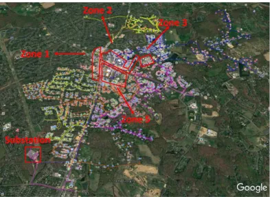
Nested microgrids refer to multiple microgrid zones within the microgrid system that can be operated independently in islanded mode and optimized as a portfolio when grid-connected. This concept is brought based on the fact that the vital services and facilities, such as fire departments and hospitals, are usually dispersed across a wide area in the community. Figure 1.6 shows Olney Town Center is such kind of community with critical services scattered all over the region. In the architecture of nested microgrids, services that are both geographically and electrically close are grouped into one control node and the services in the whole area can be served by a cluster of control groups. During grid outage, each node would serve the facilities with their own distributed generation to increase resiliency while all the nodes would be managed together to maximize economic benefits and provide grid support during normal operations. Another advantage of the nested architecture over single microgrid for the whole area is that it takes full advantage of local underground cables and avoids the cost for undergrounding of overhead lines when overhead forms most of the local backbone systems.

(21)

9

Figure 1.6 Critical load groups in Olney Town Center [14]

1.2 Microgrid Modeling and Control

1.2.1 Microgrid Modeling [15]

A microgrid system usually includes local distribution feeders, distributed energy resources (DERs), loads, reclosers and switches, power electronic interfaces, control and protection systems, and so on. To investigate system characteristics, perform power system analysis and apply control techniques, a microgrid model is required and it should be able to accurately reflect the dynamics of the real-world system.

(22)

10

modeling, there are a few typical representations of DERs that are widely used and proves effective in microgrid system modeling. A description of microgrid system models and component models are introduced in Chapter 2.

1.2.2 Microgrid Control

The microgrid control system is the key to ensure reliable, secure and economical operation of microgrids in either grid-connected or islanded mode so that the microgrid appears as a controlled, coordinated unit to the upstream network. Several most relevant challenges in microgrid control include [16]:

Stability issues: Local oscillations may emerge from the interaction of control systems of DG units. Moreover, the transition between grid connected and islanded mode needs to be done seamlessly.

Low inertia: Unlike bulk power systems where a high number of synchronous generators ensure a relatively large inertia, microgrids might show a low-inertia characteristic since the energy capacitors store is far less than energy stored in rotary shaft of the generators. The low-inertia characteristic in the system can lead to severe frequency deviations in islanding mode when there’s only a small mismatch between load and generation, especially when no appropriate control mechanism is implemented.

Uncertainty: The uncertainty of parameters, such as load profiles and weather forecasts, in microgrids is higher than that in bulk power systems due to a reduced number of loads and highly correlated variations of available energy resources. The coordination among different DERs becomes more challenging especially in isolated microgrids.

Desirable features of microgrid control systems include [16]:

Economic dispatch: An appropriate or optimal dispatch of DERs participating in the operation of a microgrid can significantly reduce costs, or increase profits with taking into account other factors like reliability, system efficiency and GHG emission.

Transition between modes of operation: The microgrid should be able to operate in both grid-connected and islanded mode, including a smooth transition between them. Different control strategies might be defined for each mode of operation.

Frequency/Voltage Control: Especially during islanded operation where system stability is sensitive to active/reactive power imbalance, DERs in the microgrid should be able to regulate voltage and maintain frequency within permissible range.

(23)

11

A full description of microgrid control functionality can be found in ORNL use cases, which are discussed in Appendix C.

1.3 Project Background

The work described in this thesis is part of the Olney Town Center Microgrid Project awarded by Department of Energy. The main purpose of the project is to research, develop, model and test a microgrid control system that is able to provide highly resilient electricity services for the Olney Town Center area, located at Montgomery County, Md. The project is studying how such a microgrid would operate in different scenarios in accordance with State and Federal goals.

The Olney Town Center serves as a critical community hub and lifeline, including a hospital, two schools, police and fire stations, a water tower, and other vital services within one square mile. Even though PEPCO, the local utility, has taken many steps to harden the grid, major equipment can be still damaged by storms and other events, resulting in an extended outage. These attributes make the Olney Town Center a good prospect for an advanced community microgrid. A high resilient microgrid at Olney Town Center will provide safety and security values by ensuring the community’s ability to provide emergency and essential services during and after an emergency or other outage-causing event.

To manage the nested microgrid, a microgrid controller, namely GreenBus, is designed by the team from Green Energy Corporation to integrate renewable energy resources, natural gas CHP units, BESS, and DSM technologies in near-real-time optimization schemes. The GreenBus system is expected to have the capability of improving reliability measure SAIDI by 98%, while increasing efficiency by at least 20% and reducing GHG emissions by 20% or more.

(24)

12

1.4 Contents of Thesis

The thesis mainly discusses microgrid model design and validation, microgrid controller test plans and evaluation methodology, test environment setup, and how test results are analyzed.

(25)

13

Chapter II. Olney Microgrid Testbed

As is mentioned in Section 1.3, the Olney Town Center Microgrid Project focuses on the development of a microgrid control system capable of providing highly resilient electricity services for critical facilities. After the microgrid control system is designed and developed, its functionalities need to be validated through a rigorous laboratory emulation.

The Olney Microgrid testbed, which provides a testing environment for the purpose of validation and evaluation of microgrid controller, is built based on OPAL-RT simulator. Opal-RT provides a distributed real-time simulation platform that can solve power system equations fast enough to continuously produce output conditions that realistically represent conditions in the real network. Because the output is real time, the simulator can be connected directly to power system control equipment and protective relay equipment or interfaced with external equipment or emulators of individual grid subsystems such as distributed generation or energy storage. Therefore, a variety of microgrid control scenarios can be evaluated through a mix of simulation and interfaces of microgrid components.

The FREEDM team has developed a multiple-zone microgrid system model that contains microgrid component prototypes for PV, BESS, and load and NG-CHP units, to emulate the local distribution network. Section 2.1 focuses mainly on the configuration of local distribution systems and microgrids. Component models as well as system models are discussed in Section 2.2. In Section 2.3, the whole test environment is introduced. Finally, verification results of testbed communication are shown in Section 2.4 to demonstrate that the testbed is successfully interfaced to the microgrid controller.

2.1 Overview of Olney Microgrid Design [17]

(26)

14

Figure 2.1 Olney Town Center microgrid zones

(27)

15

Table 2.1 Mapping on feeders to microgrid zones

Zone 1 Zone 2 Zone 3 Zone 5

Feeder 15119 √ × √ √

Feeder 15125 × √ √ √

Feeder 15126 √ × × ×

Feeder 15129 × × √ ×

There are four feeders, all of which are connected to the 13.2 kV substation, serving the Olney microgrid zones. Figure 2.2 shows the GIS information of the distribution feeders, showing that all of four microgrid zones are closer to the end of the feeders. Each feeder serves one or more than one zone and each microgrid zone consists of sections from one or more feeders. The mapping information is described in Table 2.1.

There are several special considerations for microgrid designs. Those considerations include Load Criticality, Resource Portfolio and Grid Reconfiguration, which are discussed further below.

2.1.1 Load Criticality

The primary objective of the Olney microgrid is to provide resilient electricity for critical services, so the selection of critical loads is necessary and needs to be based on some criteria. In the Olney Town Center area, there are a high density of loads that are critical to health, safety and vitality of the Olney community. There also exist substantial loads that provide convenience and shelter and other services that help maintain the community during long-duration outage events, with small loads that generally do not impact the community. Four levels of load criticality are defined as below:

High – important public safety and life-related services that must remain available and continue operations throughout the whole event and even the aftermath;

Medium – critical services that become important within the next 8 to 24 hours from the beginning of the event;

Low – critical services that become important within two days;

Optional – additional retail and other facilities, especially restaurants that can serve the community in the aftermath of the event.

(28)

16

Table 2.2 Critical load groups vs noncritical load groups Microgrid Zones Critical Load kW Peak Critical Load kW Avg Noncritical Load kW Peak Noncritical Load kW Avg Total Load kW Peak Total Load kW Avg

1 1,158 390 133 27 1,291 417

2 1,758 961 225 59 1,983 1,020

3 2,611 1,736 0 0 2,611 1,736

5 2,040 1,054 37 12 2,077 1,066

Total 7,567 4,141 395 98 7962 4239

2.1.2 Resource Portfolio

The size of generation and storage is chosen based on all the following assumptions:  accommodate the critical loads within the microgrid boundary

 support all the critical loads in an island  support use of flexible load as a resource

 support use of utility grid energy supplies as a variable resource where economically beneficial

Table 2.3 summarizes the total microgrid resource portfolio.

Table 2.3 Olney Town Center microgrid resource portfolio

Resources Total kW capacity Description

NG Engine-based CHP 3,480 2*762 kW+2*358 kW+ 5*248 kW

with 20T and 30T absorption chillers Solar PV 1,827 Rooftop PV arrays of various site Battery Energy Storage 730 Li-ion community energy storage

units

NG Generator 150 2*50 kW+2*20 kW natural gas

engine generators as base generation supplement to the CHP units

Total 6,187

2.1.3 Grid Reconfiguration

(29)

17

Since the control system is designed for nested microgrids, which operate as a portfolio when grid-connected and as separate islands upon loss of the distribution system, it is of great importance to know the PCCs of each zone. In the case of Olney circuits, each microgrid zone is assumed to have two types of PCCs: one is at the head of the zone and the other at the tail. The locations of head and tail breakers as well as tie switches can help determine logical PCC locations. Since some of the zones consist of circuits from different feeders, each zone has at least two PCCs. A detailed microgrid system reconfiguration is discussed in the Section 2.2.2.

2.2 Olney Microgrid Modeling

What makes a good microgrid system model? First of all, the test system should be equivalent to the original circuits with the same operating characteristics on buses-of-interest. Then, regarding microgrid components modeling for DERs, loads and transformers, the models that are developed should accurately reproduce the dynamic behaviors of the real world devices. Now that there are a large number of similar elements in the microgrid system under study, the prototype MATLAB/Simulink model is derived for each component. If the modeling for one component is straightforward, the built-in models in Simulink/Simpowersystems libraries are deployed but the corresponding parameters are updated to duplicate the real-world components. The further discussion on component models are given in Section 2.2.1. Section 2.2.2 focuses on how an equivalent reduced model is derived. The reason why a reduced model is required is that the original circuits are too complicated, containing almost 5000 components. Therefore, duplicating the detailed model is time-consuming. Besides, from the simulation standpoint, it’s intractable to process a large scale system at a high time resolution via real time simulators.

2.2.1 Component Model Functionality

Dynamic models are developed in the MATLAB/Simulink environment for photovoltaic (PV) systems, load groups, combined heat and power (CHP) units and battery energy storage systems (BESS) based on the real-life commercial products or existing researches. The models are used for studies on various operating modes of the microgrid controller. To represent the real-world microgrid components as accurately as possible, they are validated by a combination of real-world data as well as established component models. The details of modeling validation approach are described following the discussion on model functionality.

2.2.1.1 PV Systems

Modeling Approach

(30)

18

as a three phase controllable current source importing power to the grid. The power generated can be controlled to follow any given PV profile.

The block diagram is shown in Figure 2.3. The PV model can be attached to any bus in the grid and can inject power to follow a pre-defined, dynamically changing PV profile. In Figure 2.3, the ‘Enable’ variable (1 for on and 0 for off) controls the status of the PV. The output power from PV system is measured and logged by a three-phase V-I meter.

Figure 2.4 shows a general structure of the PV system model. Three phase voltage measured at the attached bus is transformed into the dq0 reference frame so that Vq=0. Based on the relationship: P=Ud*Id and Q=-Ud*Iq, the injected active and reactive power can be controlled by controlling the injected currents on both d-axis and q-axis. Also, because the model uses measured terminal voltage in the dq0 reference frame, in conjunction with a phase lock loop controller to determine the correct system frequency, the model is suitable for grid-connected and islanded simulations, where the frequency may vary.

The power reference used for PV system are all real world PV profiles and processed outside the model.

Figure 2.3 PV system block in Simulink

(31)

19

Functionality

 Use real-world 1-minutes solar data to create a solar radiation database;  Use interpolation to generate real-time database;

 Contain 3 PV profile day types: Sunny, Partial Cloudy, Cloudy;  Allow random selection of solar profiles;

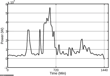
 Allow the effect of storms and clouds to be added at designated time intervals. Verification

The model is verified by feeding a random real world PV profile shown in Figure 2.5 to the model. The measured PV system power output is shown in Figure 2.6. We conclude that the model successfully emulated the real world power PV profile reference.

Figure 2.5 Referenced real world PV profile

Figure 2.6 Simulated PV system output power

0 720 1440

0 0.5 1 1.5 2 2.5 3 3.5

4x 10

5 Time (Min) P o we r (W )

0 720 1440

0 0.5 1 1.5 2 2.5 3 3.5

4x 10

(32)

20

2.2.1.2 Load Group

Load groups are modeled as a three-phase controllable current source extracting power from the grid. The extracted power can be controlled to follow any given load profile.

The model is developed in Simulink and the block diagram is shown in Figure 2.7. The model can be connected to any bus in the grid to emulate electric demand. The power flowing from grid to load group is measured as logged data. The power reference used for load groups are all real world load profiles and processed outside the model.

Figure 2.8 shows a general structure of the load group model. The modeling approach is exactly the same with PV systems. The only difference is that in this case, the power reference needs to be negative so that the direction of power flow is from grid to the current source.

Figure 2.7 Critical load groups block in simulink

Figure 2.8 Critical load groups general structure

(33)

21

Functionality

 Hourly load data provided by PEPCO and additional 15-minute residential load data based on PNNL field demos;

 Use interpolation to generate real-time database;  4 day types: Spring, Summer, Fall and Winter;  4 load priorities: High, Medium, Low, Optional;  Allow selection of load profiles in real-time;

 Allow control set points for load shedding and modulation;  Allow any level of reactive power.

Verification

The model is verified by feeding to the model a real world load profile provided by PEPCO, shown in Figure 2.9. The measured load group power output is shown in Figure 2.10. We conclude that the model successfully emulated the real world demand profile reference.

Figure 2.9 Referenced real world load profile

Figure 2.10 Measured load group input power

0 720 1440

-1 0 1 2 3 4 5 6x 10

5 Time (Min) P o we r (W )

0 720 1440

-1 0 1 2 3 4 5 6x 10

(34)

22

2.2.1.3 CHP Unit

The CHP unit is composed of a 250 kW gas fired micro-turbine, a synchronous generator and an absorption chiller. The micro-turbine consumes the natural gas as the fuel, and by burning the fuel it generates mechanical power to drive the synchronous generator. The generator then provides electrical energy to the load and grid. As a byproduct, the exhaust heat coming out of turbine can be recycled through the absorption chiller to supply cooling or heating loads. Figure 2.11 shows the block diagram of the CHP unit.

Figure 2.11 Block diagram of a CHP unit

Figure 2.12 shows the dynamic model of the CHP unit developed in Simulink. The micro-turbine unit consists of governor control, temperature control, acceleration control, fuel system, compressor and turbine, as shown in Figure 2.13. Details of simulation parameters regarding the micro-turbine block can be found in [18]. The synchronous generator block consists of the excitation system and the generator.

The following equations show the exhaust heat calculation, where Qex is the amount of exhaust

heat in kW; Pfuel is the amount of fuel sent to turbine in kW; p2, q2 are coefficient constants.

Absorption chiller is simplified to be the coefficient of performance (COP), where the input is Qex and output is the cooling capacity. COP for a single-effect ranges from 0.6 to 0.8 while

COP for a double-effect ranges from 1.4 to 1.6.



,



2

 

2

 

ex fuel out out fuel out

Q  f P T  p T P q T 

 

2 out 2 out 2

p T  a T b

 

2 out 2 out 2

q T  c T d

1

  _{for CHP on} 0

(35)

23

Figure 2.12 Simulink diagram of a CHP unit

Figure 2.13 Block diagram of the micro-turbine in a CHP unit

Functionality

 Under grid-connected mode, CHP unit delivers real power to the grid based on power reference command;

(36)

24

 Under both grid-connected and islanded mode, CHP unit provides thermal energy to cooling/heating loads.

Verification

Figure 2.14 shows the steady state performance of the CHP that delivers real power to the grid based on power reference command. Note that during hour 15 to hour 19, due to the limit of ambient temperature, the CHP unit cannot output to its maximum capacity.

Figure 2.15 shows the dynamic response of CHP during the islanding event when the CHP unit regulates the frequency of the microgrid when the transition happens at 25s. The speed variation of CHP unit jumps up immediately when grid-connected mode is transitioned to islanded mode and recovers back to one per unit after 7 seconds.

Figure 2.16 shows CHP unit provides thermal energy to cooling/heating loads. The thermal energy output to heating/cooling loads corresponds to CHP output power in Figure 2.14. It can be seen from Figure 2.16 that with the set point shown in Figure 2.14, thermal load demands (orange) exceeds CHP thermal output energy (blue) in the nighttime while there is a surplus of thermal output energy during the day.

(37)

25

Figure 2.15 Speed response between transitions from grid-connected mode to islanded mode

Figure 2.16 Thermal loads versus thermal energy provided by Chiller

2.2.1.4 Energy Storage System

The Energy Storage System consists of two parts: battery equivalent model and inverter model. A high-level block diagram is shown in Figure 2.17.

Figure 2.17 Energy storage system model block diagram External

Controller

Inverter Model

Battery Equivalent

Model

3-ph Grid

Power Reference

(38)

26

Figure 2.18 Dual polarization battery model

The battery equivalent model is used to simulate the battery’s states including the battery open-circuit voltage (Voc), terminal voltage and SOC. A dual polarization battery model is deployed in this case. This is a well-established battery modeling approach [19]. The equivalent circuit is shown in Figure 2.18.

The inverter model is developed based on Schneider Electric BESS grid-connected inverters. The inverter is modeled using average modeling approach. The block diagram is shown as Figure 2.19 below.

Figure 2.19 Schneider inverter model block diagram [20]

The inverter converts the DC power provided by the energy storage to AC power at three-phase AC nominal output voltage. The model presented is intended to produce simulation results that closely approximate the response of the plant to these disturbances, and do not in any way represent the physical implementation of the specific inverter or plant control algorithms.

Frequncy 1/(1+sTff) Droop_Freq

Pref /

Vd_PCC

+ +

1/(1+sTix)

PFref tan(cos-1) /

Qref

1/(1+sTvf) Droop_Voltage

Vd_PCC

Limit

1/(1+sTPC)

dq0

abc

PLL VPCC 1

2

3 Id_ref

Iq_ref

/ Vd_PCC

++ +- PI

+ - PI ++

Id_measured

(39)

27

Functionality

 Battery operation states (SOC, Voc, etc.) are simulated and monitored using battery equivalent model;

 Three general modes of inverter operations are provided, as follows:

1. Constant Power Factor (QMODE = 1): In this mode, the desired imaginary, or reactive, current Iq_ref is varied in direct proportion to the desired real (active) current Id_ref to maintain a constant power factor, derived from the initial conditions in the power flow solution, throughout the duration of the simulation.

2. Constant Reactive Power (default, QMODE = 2): In the default mode, the desired imaginary (reactive) power stays constant throughout the simulation by varying the imaginary (reactive) current Iq_ref in inverse proportion to the terminal voltage. The value of reactive current is derived from the initial condition in the power flow solution. 3. Voltage Control (QMODE = 3): In this mode, the desired imaginary (reactive) power is dependent on the terminal voltage Vd_PCC based on the specified Q-U dead band and droop characteristic. This function becomes active if the terminal voltage Vd_PCC is outside of the specified bandwidth. In such case, the inverter’s reactive current Iq_ref varies as a linear function of terminal voltage, according to the characteristic of Figure 2.20 below. The user defines the slope and bandwidth of the Iq-V characteristic.

Figure 2.20 IQ-V characteristic of the voltage control function [20]

(40)

28

dead band and droop characteristic. This function becomes active if the frequency is outside of the specified bandwidth. In this case, the inverter’s active current Id_ref varies as linear

function of frequency. Similar to the Voltage Control mode, the user defines the slope and bandwidth of the Id-F characteristic.

Regardless of the mode of operation, current limiting is applied to Id_ref and Iq_ref to limit the

apparent current, with reactive current given priority over active current. The real and reactive components of current are aligned with the generator bus voltage angle by means of a fast acting phase locked loop (PLL).

Verification

The verification of dual polarization battery model can be found in [19].

The verification of inverter model is included in [20].

2.2.2 Distribution System Modeling

As shown in Figure 2.2, the Olney distribution circuits within the primary microgrid footprint are four feeders with thousands of electrical components. The development of a full model with such complexity requires a great deal of time and effort, and moreover, its simulation needs significant computational power. The model is designed for studying microgrid operations under different scenarios, so circuit details outside the microgrid footprint are not modeled. Considering the impact of an upstream fault on microgrid protection equipment, the upstream utility system is simplified into a Thevenin equivalent circuit. The microgrid system is kept in detail using a reduced circuit in order to reduce the modeling effort without any impact on the characteristics of microgrid system. A circuit reduction method is applied on the system and the model is developed based on a combination of resources, including utility network KMZ models, CYME models, microgrid design models, and refinements from utility engineering department.

Circuit Reduction Method [21]

(41)

29

Next, all the nodes that don’t contain load or generation are removed. Under simple cases with a single line going through the node, the equivalent line is the sum of impedances on either side. This technique is applied to the whole distribution system. If the bus is part of a network where there is a branch split or there are multiple lines, the bus will not be removed until the next iteration of reduction.

Then, an equivalent impedance is placed to represent the upstream utility network ending at microgrid head PCC, with a dummy load representing the downstream circuit from tail PCC. The reduction technique assumes that all the upstream loads, either on the backbone feeder or at laterals, are too small compared to the loads within the microgrid boundary to impact the voltage drop. Therefore, we ignore upstream loads and combine upstream laterals. Eventually, the upstream equivalent impedance equals to the sum of the impedances of the upstream backbone feeders.

For the laterals within the microgrid boundary but not between the buses-of-interest, we combine those laterals by placing their loads on the point of interconnection. For the laterals within the microgrid boundary that contain buses-of-interest, the junction points also become buses-of-interest because laterals that did not have buses-of-interest were already removed. In cases where the lateral has the buses that contain non-critical loads, these laterals can either be combined by placing all the loads on the nearest upstream bus-of-interest or be removed if the loads are small.

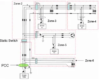
Using the method mentioned above, reduced equivalent models are derived for all the microgrid zones and feeders. The reduced one-line-diagram for the distribution feeders is shown in Figure 2.21 and a detailed model for microgrid Zone 1 is shown in Figure 2.22. The models for the rest of the zones, along with system parameters, are included in Appendix B.

(42)

30

total three PCC head breakers but only one of them is the normally-closed breaker that connects to the utility. The other PCC head breakers are normally-open interconnections to Zone 1 and Zone 2.

(43)

31

(44)

32

Verification

A short circuit analysis is conducted on the reduced microgrid model. As shown in Table 2.4, the fault currents on several PCCs match well with the results generated by running short circuit analysis on the full CYME mode. It proves that the reduced model derived using circuit reduction technique is equivalent to the original circuit.

Table 2.4 Comparison of short circuit values between full and reduced models Fault

Location

3 phase fault (kA) line to ground fault (kA)

Full Model

Reduced Model

Error Full Model

Reduced Model

Error

Substation 23.610 23.101 2% 25.610 24.906 3%

Z5-19-0 5.867 5.052 14% 3.941 3.568 9%

Z1-26-0 5.730 6.568 15% 3.926 3.622 8%

Z2-25-0 4.890 5.254 7% 3.304 3.377 2%

Z5-25-0 3.032 3.140 4% 4.527 4.977 10%

2.3 Testbed Environment Setup

As introduced in Section 2.1 and 2.2, the FREEDM Microgrid Testbed is a multiple-zone microgrid model that runs in real time on the OPAL-RT real time platform. In addition to the microgrid model, techniques are needed not only to integrate microgrid controller that remains to be validated and evaluated, but also to operate the testing in an automatic fashion. The setup of test environment is shown in the Figure 2.23.

The DNP3 protocol is utilized to emulate communication in the field for data acquisition and control. When a real-time simulation is running, the testbed supports a DNP3 outstation interface that communicates with the MMC. This allows the testbed to send out system states to the controller for monitoring and control purposes, and to receive control commands from the microgrid master controller.

(45)

33

and test-initialization parameters. If needed, the test can be automated using the Python script language supported by TestDrive.

The details about microgrid controller integration and TestDrive implementation are discussed in Chapter 4.

(46)

34

2.4 Testbed Functionality Verification

Two cases are shown in Figure 2.24 to demonstrate that the FREEDM microgrid testbed successfully integrates microgrid controller. In the first case, CHP dispatch command is sent by microgrid controller to set CHP output power from 200kW up to 240kW; in the second case, BESS charging/discharging target is sent by microgrid controller to set BESS from 10kW (discharging) to -10kW (charging). These results show that microgrid controller is able to effectively operate microgrid system model.

(a)

(b)

(47)

35

Besides the two cases mentioned above, Figure 2.25 shows a long-term steady state simulation where the controller is dispatching CHP and BESS. The results are captured and plotted using data logging function and post-processing tools in the testbed. It shows that the current testbed has the capabilities to integrate the interface to the microgrid controller, record metrics and analyze data. Additional test results are presented in Chapter 5.

(48)

36

Chapter III. Olney Microgrid Test Protocols

3.1 Overview of Test Plan and Functional Test Requirements

The test plan defines procedures utilized for validation of the core functional requirements of the microgrid controller in order to support the performance targets set by the Department of Energy, which are defined as follows [17]:

 reducing outage time of critical loads by >98% at a cost comparable to non-integrated baseline solutions (such as an uninterruptable power supply (UPS) with backup generator);  reducing emissions by >20%; and

 improving system energy efficiencies by >20%.

These performance targets are to be measured during test execution of use cases that are used to define the triggers, actors, and functions required by the microgrid system and specifically the microgrid controller. The definition of use cases mainly refers to the ORNL test cases, which are included in Appendix C.

(49)

37

Table 3.1 Table of functional test cases

Primary Functional Test Cases Microgrid Modes Objectives (Metrics)

Energy Management Grid >20% reduction in emissions

>20% improvement in system energy efficiencies

>98% reduction in outage time of critical loads

Energy Management Island >20% reduction in emissions

Ancillary Services – Demand Response

Grid – Ancillary Services

>20% reduction in emissions

Ancillary Services – Power Management

Grid – Ancillary Services

>20% reduction in emissions

Intentional Islanding – Stability

Transition to Island

Unintentional Islanding – External

Transition to Island Triggered by External Faults

Unintentional Islanding – Internal

Transition to Island Triggered by Internal Faults

(50)

38

Table 3.1 (Continued)

Primary Functional Test Cases Microgrid Modes Objectives (Metrics)

Island-to-Grid Transition Transition to Grid >98% reduction in outage time of critical loads

Microgrid black start Startup Ready >98% reduction in outage time of critical loads

Cyber Security Grid >98% reduction in outage time of critical loads

3.2 Performance Evaluation Methodology for Commercial Microgrid Controller

Efficiency, reliability and emission are three primary metrics for evaluating how well a microgrid controller performs. In this section, numerical forms of these three objectives are explored and constructed with a set of necessary measurements defined. Also we illustrate how the metrics are computed from the perspective of testing.

3.2.1 System Energy Efficiency

Microgrid architectures will improve system energy efficiency for two reasons: (1) Since microgrid enables the integration of distributed energy resources that are located close to loads, power flows in transmission and distribution circuits are reduced, so are the losses, leading to a higher system efficiency; (2) the utilization of CHP units in microgrid application can greatly improve the total energy efficiency because waste heat previously rejected to the atmosphere is made use of to provide heat for local use, thus increasing fuel-to-electricity efficiency.

According to the efficiency target proposed by DOE, it should be demonstrated that after deployment of the microgrid and its controller, the system efficiency is improved by at least 20% from that in the baseline case. The baseline is defined as the scenarios where current electric distribution system involves no distributed generation.

(51)

39

On the generation side, the efficiency of a generator or power plant is usually expressed as a percentage of the amount of energy generation to the power transmission lines divided by the amount of energy used by the generator or the power plant. It considers the losses caused when the fuel is being converted into heat or electricity. Generally, the efficiency of a thermal power plant is around 40% [24]. Therefore, most of the systems deliver electricity to users at an overall efficiency of under 40%.

A reasonable metric for evaluating microgrid system efficiency should combine both of the concepts and is shown as below:

1

n load i

m input j

E E

 





Eload ---- Energy Consumption of Critical Load Groups;

n ---- The Number of Critical Loads;

m ---- The Number of Resources including utility;

Einput ---- Energy Input to Resources.

(52)

40

Table 3.2 Microgrid efficiency test results Baseline Efficiency Critical Load

(kWh)

Component Efficiency

Energy Input (kWh)

Grid [Test Data] 40% [Test Data]

Microgrid Efficiency Energy Production (kWh) Component Efficiency Energy Input (kWh)

PV [Test Data] [Test Data] [Test Data]

BESS [Test Data] [Test Data] [Test Data]

NG-CHP [Test Data] [Test Data] [Test Data]

Grid [Test Data] 40% [Test Data]

Average Microgrid Efficiency

[Test Data] [Test Data] [Test Data]

Efficiency Improvement

[Test Data]

To calculate efficiency metric, the simulation should capture the measurements below:  CHP output power

 CHP fuel use  PV output power

 BESS charge/discharge rate

 Grid-side imported power (baseline and microgrid)  Load consumption

3.2.2 Reliability

The DOE resiliency objective is a 98% reduction in outage time for critical loads. In our case, the SAIDI index is used as the approximation of average reliability of utility service for resiliency evaluation. The SAIDI is a measure of how many interruption hours an average customer will experience over the course of a year [25]. The formula is shown below:

/

CustomerInterruptionDurations

SAIDI hour yr

TotalNumberofCustomersServed

(53)

41

Assumptions

1. Based on utility GIS information, we assume all the microgrid zones don’t have internal reclosers except for feeder 15126 in Zone 1. For the microgrid zones that don’t have internal switches, permanent faults will be isolated based on distribution system protection schemes when they occur inside the zones.

2. If temporary fault occurs, regardless of where it is, the microgrid won’t transition to islanded mode, and disturbances seen by the customers will only depend on the locations of reclosers and protection relays. All the fuses are set to fuse savings mode. In other words, temporary faults won’t affect SAIDI values.

3. Due to lack of individual customer information, we estimate the number of customers in a load group by assuming it is proportional to load size.

4. The failure rates and MTTP on overheads and UG cables are assumed according to data in [25] and PEPCO’s average SAIDI (175.3 minutes/customer/year [17]) (See Table 3.3). 5. Microgrid zones are modeled to utilize existing as-built distribution systems and to

demonstrate reliability improvements with microgrid implementation only, before considering additional system improvements, such as segment undergrounding and internal switch additions, to achieve enhanced resilience and support a 98 percent improvement in customer reliability.

6. Natural gas service is maintained during all utility grid outage scenarios.

Table 3.3 Reliability of distribution components

Conductor Type Failure Rate (counts/mile) MTTP (hrs)

Overhead Main Lines 0.36 4

Overhead Laterals 0.36 4

UG cables 0.05 10

Fault Locations

We take Feeder 15126 in Zone 1 for example to illustrate reliability analysis. In the diagram, the UG cables are marked in blue and overheads are represented in magenta. Within the microgrid zone, there is a recloser in the middle of section Z1_26_04 and four laterals, two of which are overheads and the other are UG cables.

Four types of fault locations are considered:  Fault Location 1: Upstream Utility Circuit

(54)

42

 Fault Location 3: Section Between Z1_26_0 and Z1_26_2 on Lateral 1

 Fault Location 4: Lateral of Load 1&6&7 Between Z1_26_5 and Z1_26_6 on Lateral 2

We only consider three types of internal fault locations because the Olney outage map, shown in Figure 3.1, indicates that from 2009 to 2015 there was a small chance that a fault would happen at other locations within the zone except Location 2, 3 and 4. Therefore, we assume that failure rate is negligible at other locations which are not shown in Figure 3.1.

Figure 3.1 Outage map for feeder 15126

(55)

43

The distribution of customers is shown in Table 3.4. The number of customers is estimated based on average load consumption. Though the values seem small, they nevertheless produce weighting factors for calculating SAIDI. If there are multiple locations for one critical load group, we assume each location has the same number of customers.

Table 3.4 Customers distribution information Load Group Number The Number of

Locations

Number of Customers at Each Location

Total Number of Customers

Group 1 2 3 6

Group 3 3 8 24

Group 4 2 1 2

Group 6 1 7 7

Group 7 1 5 5

Group 9 2 3 6

Total 50

Testing Evaluation Approach

To evaluate the performance of microgrid controller on enhancing reliability, tests from three use case tests (Unintentional Islanding-External, Energy Management-Islanded, and Transition-to-Grid-Connected) will be evaluated in post-process analysis to show how many customers can still be served in the aftermath of the faults under the supervision of microgrid controller. For example, if a fault occurs in the upstream circuit, reliability is determined by whether the microgrid controller can successfully transition to islanded mode and manage resources to maintain critical load. If load modulation or load shedding is required during islanded mode, then reliability metrics will degrade. Test data showing load not served will be recorded in the format described in Table 3.5 and used to calculate outage time in various event scenarios, and those metrics will be compared to baseline results shown in Table 3.6 to produce a percentage reduction in outage time and equivalent improvement in SAIDI values.

(56)

44

prioritize investments required to assure service for critical loads, supporting the DOE objective to achieve performance outcomes at a cost comparable to non-integrated UPS/backup power solutions.

Enhanced Resilience Evaluation Approach

The test team will evaluate enhanced resilience by including a long-duration outage variation among the Energy Management – Islanded use case tests. Specifically, the test run will simulate an ice storm during the month of February, resulting in a fault at Location 1 for a duration of 10 days. Such a variation will include winter daily load patterns and low PV generation, demonstrating microgrid performance in a major storm-related outage scenario. Resilience metrics will show service maintained to critical loads during this long-duration grid outage.

To calculate reliability metric, the simulation should capture the measurements below:  Amount of loads being shed for each load group

 Outage duration for each load group

Table 3.5 Microgrid reliability test results Fault Location Number of Events MTTP (hrs)

The Number of

Customers Being Served

The Number of Customers Not Being Served

1 0.652 4 [Test Data] [Test Data]

SAIDI (min/customer/year) Target 3.5

Test Result [Test Data]

Table 3.6 Baseline performance analysis (no microgrid) Fault

Location

The Number of Events

MTTP (hrs)

The Number of

Customers Being Served

The Number of Customers Not Being Served

1 0.652 4 0 50

2 0.054 4 0 50

3 0.017 4 0 50

4 0.027 4 35 15

(57)

45

(58)

46

3.2.3 Greenhouse Gas Emission

The DOE has the objective of reducing the CO2 footprint of the microgrid area by greater than 20% from the current baseline. This reduction can be achieved by displacing energy supplies from the utility generation portfolio with distributed energy resources having greater amounts of high-efficiency clean generation (natural gas CHP) and non-emitting renewable energy resources.

There are two approaches that are widely used in electric utilities [26]:

Marginal emissions factors (MEFs) are used to quantify avoided CO2 emissions. They reflect the emissions intensities of the marginal generators in the system --- the last generators needed to meet demand at a given time, and the first to respond given an intervention. For specific regions, we calculate the change in fossil generation (G) and change in emissions (E) between one hour and the next:





1 MWh

h h h

G G G_

  

 

1

h h h

E E E _ kg

  

Using linear regression techniques, the slope of a linear regression of Eon G estimates the average MEF. This definition can be applied to a general database that contains data for multiple years, or subsets of the data. For example, monthly MEFs are obtained via using 12 separate regressions of E on G for observations in each month and daily MEFs are obtained via using 24 separate regressions of E on G for observations within a given hour.

Average emissions factors (AEFs) are widely used for evaluating the emissions of either the components or the system. In our case, the AEFs are used instead of MEFs since the marginal generator concept does not apply to our microgrid test system which has one CHP unit. The AEF metrics are derived based on the knowledge of emissions from each component and computed by dividing total emissions by total energy production for a specific time interval.

(59)

47

Table 3.7 Microgrid Greenhouse Gas test results

Baseline Grid CO2 emissions Tons/MWh Total MWh Total CO2 (Tons)

Grid 0.504 [Test Data] [Test Data]

Microgrid CO2 emissions Tons/MWh Total MWh Total CO2 (Tons)

PV 0 [Test Data] 0

CHP - NG [Test Data] [Test Data] [Test Data]

BESS 0 [Test Data] 0

NG Generator [Test Data] [Test Data] [Test Data]

Grid 0.504 [Test Data] [Test Data]

Total Microgrid emissions [Test Data] [Test Data] [Test Data]