Copyright2000 by the Genetics Society of America
Selective Mapping: A Strategy for Optimizing the Construction
of High-Density Linkage Maps
Todd J. Vision,* Daniel G. Brown,
†David B. Shmoys,
†,‡Richard T. Durrett
§and Steven D. Tanksley*
*Department of Plant Breeding,†Department of Computer Science,§Department of Mathematics and‡School of Operations Research and Industrial Engineering, Cornell University, Ithaca, New York 14853
Manuscript received June 21, 1999 Accepted for publication January 12, 2000
ABSTRACT
Historically, linkage mapping populations have consisted of large, randomly selected samples of progeny from a given pedigree or cell lines from a panel of radiation hybrids. We demonstrate that, to construct a map with high genome-wide marker density, it is neither necessary nor desirable to genotype all markers in every individual of a large mapping population. Instead, a reduced sample of individuals bearing complementary recombinational or radiation-induced breakpoints may be selected for genotyping subse-quent markers from a large, but sparsely genotyped, mapping population. Choosing such a sample can be reduced to a discrete stochastic optimization problem for which the goal is a sample with breakpoints spaced evenly throughout the genome. We have developed several different methods for selecting such samples and have evaluated their performance on simulated and actual mapping populations, including the Lister and Dean Arabidopsis thaliana recombinant inbred population and the GeneBridge 4 human radiation hybrid panel. Our methods quickly and consistently find much-reduced samples with map resolution approaching that of the larger populations from which they are derived. This approach, which we have termed selective mapping, can facilitate the production of high-quality, high-density genome-wide linkage maps.
S
INCE its inception in the early decades of this cen- gained from culling relatively uninformative genotypes,a selective sampling approach is highly desirable. To tury, genetic linkage mapping has been based on
random sampling of individuals from large recombinant that end, we have developed computational methods
for finding good mapping samples and have tested the
populations (F2’s, doubled haploids, etc.) and, more
re-cently, from panels of radiation hybrid cell lines. A ran- application of these methods to several widely used
map-ping populations, including a set of Arabidopsis thaliana dom sampling approach provides a means of mapping
with little prior knowledge about each individual. How- recombinant inbred lines (ListerandDean1993) and
the GeneBridge 4 human radiation hybrid panel (
Gya-ever, large samples of recombinational crossover sites
or radiation-induced fragmentation sites, collectively re- payet al. 1996).
A two-phase mapping approach: We propose that ferred to as breakpoints, can only be obtained by
genotyp-there be two experimental phases in the construction ing large numbers of individuals.
of a high-density genetic map: the first is to construct Since individuals differ in the number and
distribu-a high-confidence frdistribu-amework distribu-and the second is to distribu-add tion of breakpoints, different combinations of
individu-new markers to this framework. This two-phased strategy als complement one another to varying degrees in the
allows many markers to be placed on a well-measured order and position information they provide. In
princi-map with a minimum of genotyping and avoids the ple, with prior knowledge of the number and position
loss in map resolution that would result from arbitrarily of breakpoints in a mapping population, it should be
shrinking mapping population size. We have dubbed possible to select a sample of individuals with a more
this strategy selective mapping. Similar strategies have desirable distribution of breakpoint sites than is likely
been proposed for determining the linkage relation-in a random sample of the same size. (We discuss some
ships between markers and phenotypic variants (e.g., possible measures of “desirability” in what follows.)
Patersonet al. 1991;Darvasi1997) and selective geno-Given the magnitude of current research efforts in the
typing of human pedigrees has been employed to map
area of linkage mapping (e.g.,Wang et al. 1998), and
markers already known to be in a particular region the potential savings in throughput and expense to be
(Fainet al. 1996). However, we are aware of no previous
application of these ideas to whole-genome mapping of molecular markers.
Corresponding author: Todd Vision, USDA-ARS Center for
Bioinfor-In the first phase of the proposed strategy, the
break-matics and Comparative Genomics, 604 Rhodes Hall, Cornell
Univer-sity, Ithaca, NY 14853. E-mail: [email protected] points for each individual in the full mapping
tion are located using a limited number of the available markers, which we refer to as the framework markers. Preferably, these markers are chosen on the basis of prior knowledge concerning their even distribution throughout the genome, as measured by breakpoint density. The map constructed in this first phase, in which the framework markers are placed confidently and precisely, is referred to as the framework map. This concept has been modified somewhat from that of
Keatset al. (1991). In the second phase, the genotypes
for all subsequent markers are scored in a small sample of individuals that have been selected on the basis of the information obtained during the first phase. The data obtained in this second phase allow the mapping of new markers relative to the fixed framework. We
Figure 1.—The concept of a bin. A bin is the interval
have recently developed methods of analysis designed between the most closely adjacent breakpoints in the sample
specifically to accommodate selected samples (D. G. under consideration. This schematic shows that while deleting
one or more individuals may result in there being fewer bins, Brownand T. J.Vision, unpublished results).
Conven-this need not result in an increased maximum bin length.
tional mapping software packages may also be modified
Boundaries between shaded and unshaded areas represent
for this task.
breakpoints. Bin lengths are drawn to scale. Individuals are Map resolution:A major concern raised by selective assumed to be haploid. (A) The inclusion of all three
individu-mapping is how much of a cost one must pay in map als breaks the interval into four unequal length bins. (B)
Removing the third individual causes the loss of the smallest
resolution in return for the benefit of genotyping
mark-bin but the maximum mark-bin length remains unchanged.
ers on only a subset of the mapping population. To answer this question, and to explore ways of minimizing this sacrifice, it is necessary to precisely define map
bin length (ABL), the sum of the squares of the bin resolution.
lengths (SSBL), and the maximum bin length (MBL). We first define a bin to be an interval along a linkage
The ABL is easily minimized. It is equal to the sum group within which no breakpoints occur among any
of all bin lengths (the genome length) divided by the members of a given set of individuals but which is
number of bins. Since the first of these is constant, the bounded by such breakpoints in at least one individual
function is minimized by maximizing the number of (or by the end of a linkage group; see Figure 1). Bins
bins. Thus, the sample of k individuals out of a mapping are the smallest unit of resolution in a genetic map; two
population of size n that minimizes the ABL consists of or more loci within a single bin cannot be ordered
the k individuals with the most breakpoints, assuming relative to one another without supplementary
informa-all breakpoints are at unique positions. Unfortunately, tion. This limit to resolution is a very real problem for
this sample may contain a small number of very long
a high-density map. Ben-Dorand Chor (1997) note
bins, resulting in a considerable fraction of markers be-that it is currently impractical to construct a mapping
ing coarsely mapped. Since this is undesirable, we sug-population with sufficient breakpoint density, even for
gest that it is preferable to minimize one of the alterna-a ralterna-adialterna-ation hybrid palterna-anel, thalterna-at the relalterna-ative order malterna-ay be
tive statistics: either the SSBL or the MBL. resolved for every triplet of linked markers when the
Minimizing the SSBL is equivalent to minimizing the number of markers is much greater than 100.
expected length of the bin containing a marker chosen We define the map resolution for a given set of
individu-uniformly at random from the whole genome. To see als to be the set of the lengths of the bins in that set of
this, consider a genome of length L, divided into bins individuals. Assuming that the location of each
break-of length l1, . . . lm. A uniformly chosen marker has proba-point is unique, and that no more than one population
bility p1⫽l1/L to be in the first bin, p2⫽l2/L to be in
member has zero breakpoints, different samples of the
the second, and so on. The expected length of the bin population will also differ in the distribution of bin
containing a uniformly chosen marker isRm
i⫽1pili⫽(1/L) boundaries and bin lengths. By selecting a collection of
Rm
i⫽1l2i. Since L is constant, the expected bin length is individuals with optimal (or near optimal) map
resolu-directly proportional to the SSBL. We note that minimiz-tion for a given size, we aim to place markers with greater
ing the SSBL is not the same as minimizing the variance precision in the second phase of selective mapping than
of the bin lengths. While the two functions are similar, would likely happen using a random sample of the same
the SSBL implicitly takes into account the number of size from the same mapping population.
bins. It can be thought of as a single statistic
incorporat-Evaluation statistics:The observed distribution of bin
ing information about both the variance and the mean lengths, and thus the resolution of a genetic map, may
of the bin length distribution. be characterized by many different evaluation statistics.
the longest bin in the genome, which may be an attrac- tial functions for protein folding (e.g., Crippen 1991)
and in the design of gene expression experiments (Karp
tive prospect to some investigators. On the other hand,
we have found that minimizing SSBL maximizes the et al. 1999), among other applications. In addition to
these tools, we have also evaluated the utility of a clean-genome-wide accuracy and precision in marker
place-ment (D. G.Brownand T. J.Vision, unpublished re- up procedure designed to ensure that each member
of the chosen sample contributes to the value of the sults). We feel that both the MBL and the SSBL are
legitimate as minimization goals. Furthermore, they are objective function.
Greedy algorithms: Greedy algorithms tend to be fast
closely correlated among samples.
and to give satisfactory solutions, but can only guarantee to find a local optimum. The simplest formulation of
METHODS AND RESULTS
the greedy algorithm is as follows. To construct a sample of size k, start with an empty sample. Then, until the We first consider an idealized case, in which the
loca-tions of the breakpoints are exactly known. We are given desired sample size is reached, find the unchosen
popu-lation member that, when added to the current sample,
a population P with n members, which we label as P⫽
{1, 2, . . ., n}, and seek the best sample subset of the most improves our objective function. The underlying
hope is that these k good choices will combine to give population for a given size k.
We cannot consider all (n
k) possible samples, since this a sample that is good overall (NemhauserandWolsey
1988, p. 393). An alternative strategy is to start with number is prohibitively large for realistic values of n
[e.g., (100
30)⫽1026]. Instead, we have considered a number the entire population as the sample, and at each step,
remove the member from it that would have the least of naive heuristics, which turn out to perform rather
poorly, and have developed much more desirable algo- effect on the objective function, until the sample is of
the desired size. We did not employ this strategy because rithms using ideas from the field of discrete
optimiza-tion. it is computationally very expensive for large
popula-tions. To evaluate the quality of a possible sample, we order
all of the breakpoints in the members of the sample One can avoid focusing on a single local optimum
by incorporating a limited element of randomness into and compute the MBL, that is, the longest distance
between consecutive breakpoints (including the ends the choice of each member of the sample set. To
imple-ment a randomized greedy algorithm, choose the next of linkage groups). This statistic is our objective function;
for each sample size k, we seek the population sample sample member uniformly at random from the r choices
that would most improve the objective function for some of that size that minimizes the objective function. Later,
we consider data from real populations, where we do small value of r (e.g., 3 or 5;Resende1998). Repeat this
a large number of times, and choose the best sample not know the exact sites of the breakpoints. For such
cases, we will seek a sample that minimizes a slightly set found.
To further improve upon this scheme, we have consid-modified objective function.
Let the performance ratio of a sample be the ratio of the ered a mixed greedy algorithm that sequentially employs
two different objective functions. To build a mixed objective function value for the sample to the objective
function value for the population as a whole. Clearly, greedy sample of size k, first build a sample S1of size
k/2 by performing the greedy algorithm with the SSBL
the best possible performance ratio is 1.0, and the
per-formance ratios of all algorithms will approach 1.0 from objective function. After k/2 selections, switch to the
greedy algorithm to minimize objective function MBL, above as k approaches n.
Naive algorithms:One naive algorithm is to generate augmenting S1 until a sample S of size k is obtained.
The reasoning behind this approach is that minimizing a large number of random samples of size k and select
the generated sample with minimum objective function the first objective function forces all bins to be small,
rather than myopically focusing on the largest bin. Thus, value. A less naive algorithm is to choose the sample that
consists of the k individuals having the most break- upon switching to the MBL objective function, one has
a better starting point than if one had begun with the points. As discussed above, this latter sample is
guaran-teed to have the smallest possible ABL for a given k. MBL objective function initially. We have considered a
randomized version of this algorithm where the half However, it may be far from optimal at minimizing the
MBL or SSBL. sample S1is produced by a randomized greedy
proce-dure and the augmentation to the full sample is by a
Preferred algorithms: In addition to evaluating the
performance of these naive algorithms, we have made nonrandomized greedy algorithm. Since we have found
that this randomized mixed greedy algorithm consis-use of more sophisticated tools, including greedy
algo-rithms, integer programming, and linear programming tently outperforms simpler (nonrandomized or
non-mixed) greedy algorithms both in simulations and in with randomized rounding. Neither greedy algorithms
nor mathematical programming are new to biological real data, we only report results for the randomized
mixed greedy algorithm in our results on the MBL. We applications. Greedy algorithms have been used for
DNA sequence assembly (e.g.,Staden1979), while math- also report results using an unmixed randomized greedy
poten-Integer linear programming: poten-Integer linear program- corresponding to the midpoint of the range ( Nem-hauserandWolsey 1988, p. 127).
ming is an alternative solution method that has the
Unfortunately, integer programs can be quite slow to advantage of finding the optimal sample of size k.
How-solve, and their solution time increases quite dramati-ever, it requires a prohibitive amount of computation
cally as their size increases (Nemhauser and Wolsey
for a large population.
1988, p. 125). In this case, the solution time depends Let the objective function be MBL and consider the
primarily on the population size. While the optimal population P⫽{1, . . ., n}. To each member i of P, assign
threshold, and its associated sample, can be calculated a decision variable yi, where yi⫽1 if member i is included
for reasonably small, simulated data, this is not so for
in our sample, and yi⫽0 otherwise. The constraints on
moderate to large mapping populations. Thus, we have the variables model the requirements of the sample and
employed integer programming primarily to evaluate must be linear constraints in the decision variables. The
the performance of alternative algorithms, none of first constraint on the yi’s is that兺iyi⫽k, requiring that
which can guarantee an optimal sample. a sample of size k must be chosen. To formulate the
Linear programming with randomized rounding: Linear
second set of constraints, consider an objective function
programming, another form of mathematical program-value B and suppose that it is possible to find a sample
ming, provides a common way to work around the com-of size k that achieves this value. In this sample, the
putational intractability of integer programming. One longest distance between consecutive breakpoints is less
“relaxes” the integer programming requirement that than or equal to B. To encode this into a finite number
the yivariables are 0 or 1 and simply requires that the
of constraints, we note that the distance between any
yibe in the closed interval from 0 to 1. One then obtains breakpoint in the entire population and the next
solutions that may fractionally choose population mem-breakpoint in the sample is less than or equal to B,
bers, with the sum of the fractions still equal to k. For since each unchosen breakpoint is between two chosen
a given threshold B, we consider the following linear breakpoints, which we know are separated by a distance
program, which we call LPB:
less than or equal to B. For each breakpoint j in any of
the members of the population, let Cj,B be the set of
兺
i
yi⫽k; (4)
population members i that have a breakpoint after j
and within distance B of it. Then, for each breakpoint
兺
i苸Cj,B
yiⱖ1, for each breakpoint j; (5)
j in the entire population, at least one member of Cj,B
must have been chosen. For each breakpoint j, this 0ⱕy
iⱕ1, for all i⫽ 1 . . . n. (6)
requirement can be modeled by adding to the integer
These linear programs, without the integer require-program the constraint 兺i苸Cj,B yi ⱖ 1. Thus, there is a
ment on the yi, are much easier to solve (Chva´tal1983) sample of size k with objective function value less than
and assignments to the yi variables that satisfy these
or equal to B exactly when there is a solution to the
constraints are still valuable despite being potentially following set of constraints, which is the integer program
fractional. For example, they allow us to judge the
qual-corresponding to distance B, or IPB:
ity of a given sample. Let B*
LPbe the smallest value of B
for which LPBis feasible. Then B*LPⱕ B*, since if y is
兺
i
yi ⫽k; (1)
the 0–1 assignment that shows that IPB*. is feasible, then
y is also a feasible assignment for LPB*. Suppose, then,
兺
i苸Cj,B
yi ⱖ1, for each breakpoint j; (2)
we find a sample S with objective function value BS,
which is close to B*
LP. Then B*ⱕBS, since B*is the best
yi 苸{0, 1}, for each i⫽1, . . . , n. (3)
possible value. So B*
LPⱕ B* ⱕ BS, and if BS is close to
We say that a set of constraints is feasible if it can be B*
LP, then it must also be close to B*. Hence, the linear
satisfied by an assignment to the yi decision variables program gives a lower bound on the optimal objective
(called a feasible solution); otherwise it is infeasible. One function for the integer program.
seeks B*, the minimum possible value of B for which
In addition to obtaining lower bounds on B*with the
IPB is feasible; this is the best objective function value linear programs, one can also use feasible yiassignments
that can be attained for sample size k. An optimal sam- to the linear programs to select actual samples. Each of
ple, then, consists of the k population members for the yi will range from zero to one. If we treat yias the
which yi⫽1 is a feasible solution to IPB. Note that there probability with which we choose to include population
may be multiple feasible solutions for a given feasible member i, and we make these choices independently,
set of constraints. then the expected sample size is k. Intuitively, this
“ran-One can obtain the value of B*solving a limited num- domized rounding” scheme takes advantage of the
in-ber of integer programs using a bisection search strat- formation in the yi. If yi is near one, one is likely to
egy. To do this, one maintains a range of values in which include member i; if it is near zero, it will probably not
B*may fall and cuts the range in half at each step based be included in our sample (RaghavanandThompson
it greedily until it is of size k; if too large, remove the 5 min and was almost entirely devoted to solving the linear programs.
sample members whose deletion has the least impact
on the objective function until the sample is of size k. The results are shown in Figure 2A. The figure shows,
for several algorithms, the mean performance ratio (the Repeat the process many times and choose the best
sample set found. MBL of the sample divided by the MBL of the entire
population) for the samples found of a given size. We Integer and linear programs designed to minimize
SSBL, as opposed to MBL, are too computationally in- also computed the optimal samples of each size using
integer programming. The randomized mixed greedy tensive to be practical even for moderately sized data
sets. Therefore, we report only mathematical program- and linear programming with randomized rounding
so-lutions were nearly indistinguishable from one another ming results for the MBL objective function.
Post-selection clean-up: In optimizing the MBL, it is often and were extremely close in MBL to the optimal samples found by integer programming.
possible to improve the samples chosen by the greedy
and randomized rounding algorithms described above On the other hand, the two naive algorithms
(choos-ing the best of 50 random samples and choos(choos-ing the by adding a clean-up routine. The longest interbreakpoint
interval of a given sample is defined by only two sample sample containing the most breakpoints) required
sam-ples approximately twice as large, or larger, than would members: the member that includes the first breakpoint
of that interval and the member that includes the sec- be optimal for a given performance ratio. For example,
the mean performance ratio of the samples from the ond breakpoint. Taking advantage of this fact,
imple-ment a clean-up routine by looking at a provisionally randomized mixed greedy algorithm of size 25 was 1.27;
this performance ratio was not achieved until size 52 selected sample, in the order in which the individuals
were added, and removing individuals whose deletion when the best of 50 random samples was selected and
until size 68 when the population members with the does not increase the maximum bin length. Then restart
the greedy algorithm and augment the now incomplete most breakpoints were selected. We examined whether
choosing the best out of a larger set of random samples sample until it reaches size k. Repeat this process until
removing any single member from the sample would (1000, instead of 50) made a qualitative difference to
this conclusion and found that it did not (results not increase the MBL. In the experiments we report below,
the randomized mixed greedy and randomized round- shown). Figure 2A also shows the average, as opposed
to the best, performance ratio among 100 random sam-ing algorithms both include this clean-up routine.
ples. If a researcher were to randomly cull a population comparable to this one, for whatever reason, this is the
Simulated populations with exactly specified breakpoints
sacrifice in mapping resolution that would result. As can be seen from the comparison of the average and the We evaluated the performance of our sample
selec-tion algorithms on simulated data with exactly specified best random samples, the variability among the random
samples was small compared to the distance between breakpoints. We looked for the minimum sample sizes at
which these algorithms found samples whose objective these samples and those selected by the more
sophisti-cated algorithms. function values were close to the objective function
value for the full population. We then chose samples The addition of the clean-up routine made a
substan-tial contribution to the quality of the samples chosen, of constant size from populations of increasing size.
This was done with the twofold aim of evaluating the particularly for the randomized rounding routine. The
cleaned randomized rounding samples had a perfor-sensitivity of algorithm performance to population size
and providing some guidance as to how large a popula- mance ratio 12.6% closer to 1.0 than uncleaned
sam-ples, when samples of all sizes were considered. We tion size should be used in constructing a framework
map. All of our test codes were implemented in Matlab also found that, in the absence of the clean-up routine,
samples chosen by randomized rounding had signifi-5.3 (Mathworks, Natick, MA) and run on a Sun Ultra
Sparc 10 workstation. Our linear and integer programs cantly higher MBL than samples chosen by the
random-ized mixed greedy algorithm. When the clean-up rou-were solved with CPLEX 4.0 (CPLEX Optimization,
In-cline Village, NV), an industrial mathematical program- tine was added, the performance ratios of samples
chosen by these two algorithms became nearly indistin-ming package.
Fixed population size with increasing sample size:In guishable. While the clean-up routine was appended to the end of these two algorithms and not the others, we
our first set of tests, we simulated 10 F1 recombinant
populations of 100 haploid organisms with a genome found that this difference was not wholly responsible
for the striking separation between the two classes of length of 1000 cM. Breakpoint sites were generated by
simulating, for each organism, a homogeneous Poisson algorithms; the randomized rounding and randomized
mixed greedy selected samples had consistently lower process with mean inter-breakpoint distance of 100 cM.
For all sample sizes, the randomized greedy algorithms performance ratios than samples chosen by the other
algorithms even in the absence of a clean-up routine ran in less than 10 sec. The computation time for the
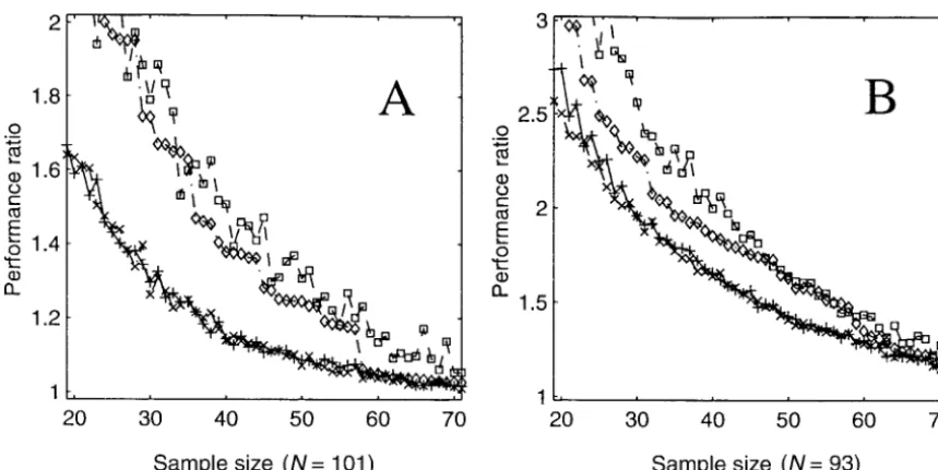
Figure2.—Optimization for the maximum bin length in simulated populations with exact breakpoint placement. The haploid F1 population size is 100 and the simulated map length is 1000 cM. (A) Shown are the average performance ratios, over 10 replicates, for samples of varying sizes chosen by each of six different algorithms. The performance ratio is defined as the ratio of the maximum bin length in the selected sample relative to that for the population as a whole. (B) Shown are the maximum bin lengths in samples of size 30 chosen from populations of variable size using several different algorithms. Plotted is the maximum bin length value averaged over 50 simulated populations. Integer programming results are not shown. (⫻) Random-mixed greedy; (⫹) randomized rounding; (䉫) most breakpoints; (䊐) best of 50 random samples; (䉭) average random sample; (—, in A) the integer programming, or optimal, solution; (䊊, in B) the linear programming lower bound; and (䊉, in B) the whole population. Note that the random-mixed greedy and randomized rounding solutions approach the optimal solution (in A) or the lower bound (in B) and greatly outperform the alternative heuristic algorithms.
Increasing population size with fixed sample size:In ized mixed greedy and randomized rounding algo-rithms performed quite well. In contrast, the best-of-50-the second set of simulations, we examined best-of-50-the effect
of increasing the size of the mapping population while random-sample algorithms selected samples of equally
poor quality at all population sizes. Interestingly, the holding the sample size fixed. Better samples potentially
exist within larger populations but, because the search algorithm that chose the population members with the
most breakpoints improved only slightly in performance space expands rapidly with increasing population size,
it might be more challenging to find them. Further- as the population size increased.
The randomized rounding and randomized mixed more, the map resolution of the best sample of a given
size may not increase as rapidly as that of the whole greedy algorithms improved in an absolute sense as the
population size increased; however, their performance population. Thus, we desired to measure both the
abso-lute and relative map resolution as a function of popula- ratios slowly increased, as well. In other words, the MBL
of the whole population decreased faster than the tion size.
We simulated 50 haploid recombinant F1populations MBL of selected samples of fixed size. The performance
ratio of the linear programming lower bound B*
LPalso
each of sizes 50, 75, 100, 125, and 150, with genome
length 1000 cM, as before, and generated samples of increased (Figure 2B), suggesting that the randomized
rounding and randomized mixed greedy samples were size 30 from each of these populations. The results are
shown in Figure 2B; the figure shows, for each popula- still close to optimal for their size.
The MBL of the population as a whole approximately tion size, the MBL in samples generated by each of
the algorithms. Due to the computational speed of the halved as the population size doubled. (This can be
explained by noting that the entire population of N randomized greedy algorithm, we were able to select
samples of size 200 from populations as large as 500 in individuals is equivalent to a sample from a single
homo-geneous Poisson process with mean inter-event distance only a moderate amount of computer time. The linear
programming algorithm was practical for populations of 100/N cM). An important consequence of this
non-linear relationship between population size and map of fewer than about 300. The integer program did not
converge within 24 hr for populations of size 125 and resolution is that, even in the absence of selected
sam-pling, improvements in map resolution become increas-150, so these results were not obtained; for clarity, the
integer programming results are not shown in Figure 2B. ingly more modest as the population size grows.
random-Figure4.—Cumulative bin length distributions under
dif-Figure 3.—Optimization for the sum of squares of bin
ferent sample selection algorithms. The haploid F1population lengths in simulated populations with exact breakpoint
place-size is 100 and the simulated map length is 1000 cM. The ment. The haploid F1population size is 100 and the simulated
fraction of the genome found in bins of less than a given bin map length is 1000 cM. Shown are the performance ratios
length is shown for samples of size 30 found using four differ-for one replicate, in samples of varying size, chosen by four
ent sample selection methods and for the whole population. different algorithms. The performance ratio is defined as in
(䊉) Whole population; (䉮) random greedy (minimizing sum Figure 2. (⫻) Random greedy; (䉫) most breakpoints; (䊐)
of squares of bin lengths); (⫻) random mixed greedy (min-best of 50 random samples; (䉭) average random sample.
imizing maximum bin length); (䉫) most breakpoints (most breakpoints (minimizing average bin length); (䉭) single ran-dom sample.
also evaluated samples chosen solely to minimize SSBL in a 100-member simulated population. Figure 3 shows
the result from this experiment, plotting the SSBL vs. at one extreme and that of a single random sample at
the other. the mapping population size for the best of 50 randomly
chosen samples of each size, the sample chosen to have Application to existing mapping populations:We
ap-plied these algorithms to a number of different existing the most breakpoints, and the sample found by the
greedy randomized algorithm. (A mathematical pro- mapping populations. We report on these results in
detail for two populations constructed in very different gramming formulation is computationally impractical
with this objective function.) The differences in sample ways. The first of these is a recombinant inbred (RI)
population derived from a cross between A. thaliana quality among the algorithms are not as pronounced
as for MBL, but it is still clear that the randomized ecotypes Columbia and Landsberg erecta (Lister and
Dean 1993; http://nasc.nott.ac.uk/RIdata). We
ana-greedy samples are of higher quality than can be found
by naive methods. lyzed 101 lines scored for 261 of the identified
frame-work markers spaced at an average of 2.0 cM apart. The We were also interested in the distribution of the bin
lengths in samples chosen to minimize ABL, MBL, or total map length in this population is 513.1 cM. Since
there is a twofold expansion of crossover frequency as SSBL. Figure 4 shows the cumulative fraction of the
genome found in bins of various lengths for selected a result of the repeated selfing of these lines (Haldane
andWaddington1931), the Arabidopsis RI population samples of size 30 chosen from the same 100-member
simulated population. For reference, the distribution is closely comparable to the simulated haploid
recombi-nant F1population, for which the total map length was
for the entire population is shown. Despite there being
many small bins in the sample containing the most 1000 cM. The second mapping population that we
con-sider in detail is the GeneBridge 4 radiation hybrid breakpoints, much of the genome is still represented
by large bins. The samples minimizing MBL and SSBL (RH) panel of 93 hamster cell lines, each retaining
about 32% of the human genome (Gyapayet al. 1996).
concentrate more of the genome in small to
moderate-length bins. Unlike the MBL sample, the SSBL sample Due to several large gaps between the framework
mark-ers in the RH map, we divided the linkage groups with does not accumulate bins that are just shy of the
maxi-mum length. On the other hand, the SSBL sample does gaps of length greater than 25 centirays (cR), or a
popu-lation breakage frequency of 25%, into linkage groups have a slightly longer maximum bin length than the MBL
sample. The ABL, MBL, and SSBL bin length distribu- within which all framework intervals were less than or
estimation more precise. However, it does not preclude further modification to handle the imprecisely specified breakpoints of the RI and RH data. For the randomized the occurrence of bins greater than 25 cR since bins
may span multiple framework intervals. We found in rounding algorithm, we treat a feasible set of yivariables
to a very closely related linear program as the probability simulation experiments (results not shown) that
intro-ducing a small number of long (greater than 40 cM) that each population member is either rejected or
ac-cepted to the sample and then greedily adding to the gaps into a simulated framework map had only a small
effect on the ability of our algorithms to find samples sample until it is of full size. See appendix b for the
differences between the linear program solved in the exact with small MBL. But there were many such gaps in the
human data set, and we chose to be conservative. In case and that needed for the stochastic case. Integer
programming is not appropriate in this case, as our total, we analyzed 55 human linkage groups with a map
length of 10,866 cR. In addition to these, we analyzed previous integer programming model assumed
knowl-edge of exact breakpoint placement. We note that the a number of other published mapping data sets.
Unlike the simulated populations, in which break- linear programs solved in this case are much smaller
than for the exact case and can easily be solved for points could be precisely localized, the marker
geno-types in the real data sets allow us only to identify those populations of size greater than 300.
intervals bearing odd numbers of breakpoints. Although unobserved breakpoints undoubtedly occur in the
map-Results for Arabidopsis, human, and other data sets
ping populations under consideration, they do not
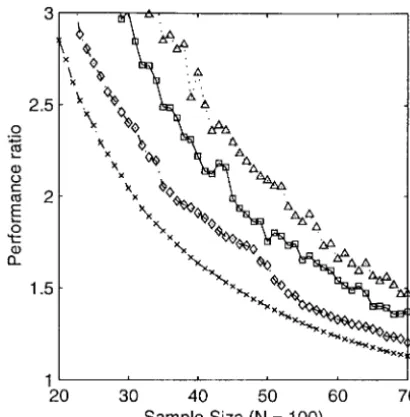
con-tribute to our choice of a sample. For each observable For the Arabidopsis data (Figure 5A), we found that
the randomized mixed greedy and randomized breakpoint, we assume that there is exactly one
break-point uniformly distributed between the flanking mark- rounding algorithms both performed well, although not
as well as on simulated data, and they greatly outper-ers and that no breakpoints occur in intervals having
identical flanking markers. Further, we assume that the formed the naive algorithms. For example, the
random-ized mixed greedy algorithm found a sample of size 30 sites of breakpoints are unique and independent of one
another. with performance ratio less than 1.3; to achieve the
same performance ratio with a sample containing those This conforms to our earlier assumption that
break-point sites are generated by independent Poisson pro- lines with the most breakpoints required 45 individuals.
For samples of size 30, the randomized mixed greedy cesses. It also assumes that map distances are additive,
which is ideally the case. Since nonadditivity of map and randomized rounding algorithms ran in less than
5 min. Much of this time was occupied in repeated distances, and the related phenomenon whereby the
map length expands with the addition of new markers, evaluations of the objective function via simulation
dur-ing the greedy additions. are largely due to the use of an inappropriate mapping
function (Liu1998) and/or the accumulation of geno- For the radiation hybrid data (Figure 5B), we found
that both the differences among the algorithms and the
typing errors (LincolnandLander1992), sample
se-lection should be preceded by careful error checking improvements obtained by selective sampling were less
dramatic than for the recombinant inbred data. While and rigorous analysis of framework marker data.
Updating the algorithms: Given the uncertainty in the shape of the relationship between performance ratio and minimum sample size was similar for both data sets, precise breakpoint location, we wish to minimize the
expectation of the MBL or SSBL, under the assumption the samples required to achieve a given performance ratio were approximately 50% larger for the human that known breakpoints are uniformly and
indepen-dently distributed within framework intervals. A closed- data. In addition, the superiority of the randomized
mixed greedy and randomized rounding algorithms di-form di-formula for E (MBL) is not readily available. So,
to evaluate the MBL objective function, we generate minished as the performance ratio approached 1.0. Still,
for modest sizes, we did experience significant improve-100 replicates of the population in which all breakpoints
have been instantiated (i.e., randomly resolved to exact ments. A sample of size 47 was obtained by both the
greedy and linear programming algorithms with a per-sites). We compute the mean quality of our chosen
sample for these replicates using the same objective formance ratio less than 1.5. By comparison, the
same-sized sample containing those cell lines with the most function as in the simulations described above, where
breakpoints were known with precision. For E(SSBL), visible breakpoints had a performance ratio greater
than 1.7. we have derived a closed-form solution given known
marker sites and a known number of breakpoints be- The superior performance of selective sampling in
the Arabidopsis population appears to be due to the tween consecutive markers. For a full derivation of
this formula, see appendix a. Accordingly, our mixed smaller number of breakpoints per individual.
Compari-sons of simulated data with comparable average break-greedy algorithm selects the first half of the sample
without the need to randomly resolve the breakpoint point densities (10 or 100 per individual) gave
qualita-tively the same results as the Arabidopsis and human locations many times over, thereby improving both the
accuracy and the speed of the algorithm. data, respectively (results not shown). That is, for the
Figure5.—Analysis of existing mapping populations. Shown are the performance ratios (of maximum bin length) for samples of varying size chosen by four different algorithms: (⫻) random-mixed greedy (minimizing maximum bin length); (⫹) randomized rounding (minimizing maximum bin length); (䉫) most breakpoints; and (䊐) best of 50 random samples. (A) The Lister and Dean Arabidopsis recombinant inbred (RI) population. Population size is 101 and map length is 513.1 cM. (B) The Genebridge 4 human radiation hybrid (RH) panel. Population size is 93 and map length is 10,866 cR.
sizes were required for a given performance ratio and much smaller sample can be selected for subsequent
the sizes needed to approach a performance ratio of mapping that very nearly minimizes the necessary
sacri-1.0 were similar for all of the algorithms, including the fice in map resolution. Two computationally efficient
naive ones. The explanation for this appears to be as algorithms have been found that are successful in
find-follows. Consider a long genome composed of some ing samples with small maximum bin length. The first is
number of short genomes concatenated end to end. a greedy algorithm that employs two objective functions
The breakpoint distributions in the short genomes are sequentially, first minimizing the sums of the squares
independent and the MBL of the long genome is the of the bin lengths and then minimizing the maximum
maximum of the MBL among the short genomes. For bin length. It also exploits randomness to search a large
any sample, the performance ratio for the long genome space of possible good samples. The second algorithm
will be the worst performance ratio achieved for any of involves linear programming with randomized
round-the short genomes. This will clearly be worse than round-the ing to convert fractional assignments into integral ones.
average performance ratio among the short genomes. Sample sets from both algorithms are improved by the
Hence, the gain to be realized by selective sampling for inclusion of a clean-up routine that disposes of members
MBL is diminished by increasing breakpoint density. that do not contribute to the quality of the sample and
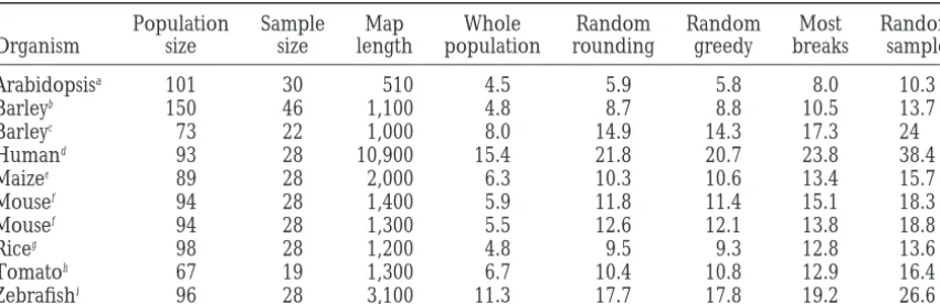
Table 1 shows the results of selective mapping for greedily replaces them with other selections that do.
maximum bin size using 10 data sets, including the two The greedy and linear programming algorithms
dramat-described above. Samples were chosen, using several ically outperform more naive alternatives such as
choos-different algorithms to be approximately 30% the size ing the individuals with the most visible breakpoints or
of the base population. The randomized rounding and choosing the best of a collection of randomly generated
randomized mixed greedy algorithms performed com- samples. Furthermore, the linear programming and
parably to one another and outperformed the most greedy algorithms find samples that are within a few
breakpoints sample in all populations. For the random- percentage points of the optimal sample for a given
ized greedy algorithm, performance ratios ranged from size, as indicated by comparisons with the integer
pro-1.29 to 2.2. While maximum bin length was significantly gramming solution for simulated data. For an
alterna-correlated with genome length (for the randomized tive objective function, the sum of the squares of the bin
greedy algorithm, ⫽ 0.8, P ⬍ 0.005), performance lengths, the samples we find by using the randomized
ratio was not. greedy algorithm are also superior in map resolution
to random samples.
The radically different origins of the breakpoints in
DISCUSSION
the various recombinant populations examined here and the GeneBridge 4 human radiation hybrid panel We have shown that, given genotypic data for a limited
TABLE 1
Maximum bin size in samples from a variety of datasets
Population Sample Map Whole Random Random Most Random
Organism size size length population rounding greedy breaks sample
Arabidopsisa 101 30 510 4.5 5.9 5.8 8.0 10.3
Barleyb 150 46 1,100 4.8 8.7 8.8 10.5 13.7
Barleyc 73 22 1,000 8.0 14.9 14.3 17.3 24
Humand 93 28 10,900 15.4 21.8 20.7 23.8 38.4
Maizee 89 28 2,000 6.3 10.3 10.6 13.4 15.7
Mousef 94 28 1,400 5.9 11.8 11.4 15.1 18.3
Mousef 94 28 1,300 5.5 12.6 12.1 13.8 18.8
Riceg 98 28 1,200 4.8 9.5 9.3 12.8 13.6
Tomatoh 67 19 1,300 6.7 10.4 10.8 12.9 16.4
Zebrafishi 96 28 3,100 11.3 17.7 17.8 19.2 26.6
All distances are measured in centimorgans except for the human radiation hybrid panel, which is measured in centirays.
aListerandDean(1993). bKleinhofset al. (1993). cGraneret al. (1994). dGyapayet al. (1996). eBurrandBurr(1991). fBlakeet al. (1999).
gTaguchi-Shiobaraet al. (1997). hTanksleyet al. (1992).
iPostlethwaiteet al. (1998).
variety of mapping populations. We have not analyzed and an incremental cost per genotype. With selective
mapping, the latter costs are reduced in direct propor-multigenerational pedigrees here, because of the added
complication due to breakpoints that are identical by tion to the reduction in the size of the mapping
popula-tion. For inherently serial genotyping methodologies, descent. But these could, in principle, be
accommo-dated. Our methodology does not require that any map- such as denaturing high-pressure liquid
chromatogra-phy (Underhill et al. 1997) or mass spectrometry
ping function be used to derive the framework map.
However, the assumptions made about breakpoint dis- (Griffin et al. 1997), there would also be a directly
proportional reduction in the time required to map tribution in the sample selection process are the same
as those underlying the Haldane mapping function each locus. Since mapping on the order of 5000 markers
currently requires tens to hundreds of thousands of (Haldane1919). Under these assumptions, our
meth-odology can accommodate segregating populations dollars and may take several years for a moderately
equipped lab to complete, the potential savings from
with unknown linkage phase (e.g., an F2) without further
modification. If the model is violated by the presence the application of selective mapping are considerable.
Rather than sacrificing map resolution, one could apply of interference, then fewer double recombinations
would be expected to occur between framework mark- selective mapping to a project with the aim of attaining
the finest map resolution possible given the resources ers. As a consequence, the performance of the selection
algorithms may be somewhat improved. that are available by tuning the population size, sample
size, and framework density accordingly. On the basis of these results, we propose a two-phase
mapping strategy for projects in which a very large num- Clearly, it is desirable to have a framework map
suffi-ciently dense that one may catalog the locations of the ber of markers are to be mapped on a single population.
In the first phase, the genotypes at a set of framework overwhelming majority of the breakpoints in the
popula-tion. But it would be counterproductive to make the markers are scored in the full mapping population, and
a framework map is constructed from these data. In the framework so dense that only a small proportion of the
markers remain to be genotyped in the selected sample. second phase, markers are mapped using only a selected
subset of the population and positions are inferred rela- We propose the rule of thumb that, at the very least,
framework markers should be chosen so as to be evenly tive to the fixed framework map. By adopting this
strat-egy, a near-optimal balance may be reached between spaced at intervals of less than half the length that would
be tolerated as the maximum bin length. The rationale mapping precision and genotyping effort.
Practical considerations: The cost of genotyping is for this is that if two adjacent framework intervals each contain one breakpoint, the distance between the two
dependent upon laboratory methodology (Cotton
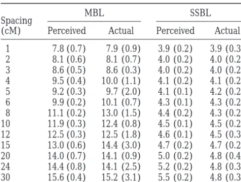
TABLE 2 number of individuals allows for an extremely large number of possible genotypic configurations. For a
Effect of framework marker spacing on map
mapping population of n individuals, in which one can
resolution of selected samples
distinguish x genotypes at each locus, there are xn possi-ble genotypic configurations. For reasonapossi-ble values of
MBL SSBL
Spacing n and x, the number of possible configurations is far
(cM) Perceived Actual Perceived Actual
larger than can be expected to occur in an actual
map-1 7.8 (0.7) 7.9 (0.9) 3.9 (0.2) 3.9 (0.3) ping population (e.g., 230 ⬎ 1 ⫻ 109). However, the 2 8.1 (0.6) 8.1 (0.7) 4.0 (0.2) 4.0 (0.2) actual number of bins in a population is limited by the 3 8.6 (0.5) 8.6 (0.3) 4.0 (0.2) 4.0 (0.2) rarity of recombinational or radiation-induced break-4 9.5 (0.4) 10.0 (1.1) 4.1 (0.2) 4.1 (0.2) points within each individual and will always be orders 5 9.2 (0.3) 9.7 (2.0) 4.1 (0.1) 4.2 (0.2)
of magnitude less than xn. It is governed both by the
6 9.9 (0.2) 10.1 (0.7) 4.3 (0.1) 4.3 (0.2)
size of the population and the type (e.g., in an F2 popula-8 11.1 (0.2) 13.0 (1.5) 4.4 (0.2) 4.3 (0.2)
tion of size n, the expected number of bins is 2n⫹ 1
10 11.9 (0.3) 12.4 (0.8) 4.5 (0.1) 4.5 (0.2)
12 12.5 (0.3) 12.5 (1.8) 4.6 (0.1) 4.5 (0.3) for a 100-cM linkage group). We have found that
multi-15 13.0 (0.6) 14.4 (3.0) 4.7 (0.2) 4.7 (0.2) ple bins with identical or near-identical genotypic
con-20 14.0 (0.7) 14.1 (0.9) 5.0 (0.2) 4.8 (0.4) figurations only occur in very small mapping popula-24 14.4 (0.8) 14.1 (2.5) 5.2 (0.2) 4.8 (0.3) tions and are not a major concern in practice (D. Brown 30 15.6 (0.4) 15.2 (3.1) 5.5 (0.2) 4.8 (0.3)
andT. Vision, unpublished results).
Mean and standard error (in parentheses) for samples of The problem of data analysis after the second round
30 from five simulated haploid F1populations of size 100 with of genotyping is somewhat novel, in that all distance genomes 600 cM long. Data for SSBL are divided by genome information is derived from the observed distances in length and are thus expected bin size.
the framework map and potentially large numbers of new markers, genotyped only in the selected sample, are to be placed in ordered bins. We have developed longest bin between them. If markers are spaced more
widely, then the algorithms described in this article may fast and robust methods, to be reported elsewhere, that
are appropriate to this analysis (D. Brown and T.
perform poorly in finding a sample with a desirable
breakpoint distribution. Table 2 shows the results of Vision, unpublished results). Conventional mapping
software may also be modified to order new markers simulations in which marker density was varied on
popu-lations with exactly specified breakpoints with simulated relative to the framework and to each other and to
measure distances relative to the fixed framework. genome length 600 cM, where samples were selected
on the basis of the visible marker genotypes. Measured A natural extension of selective mapping would be
to divide a very large population (of size much greater by MBL, both actual and perceived resolution varies
roughly 2-fold between the highest (1 cM) and lowest than 100) into multiple samples, each containing a
de-sirable distribution of breakpoints for a particular chro-(30 cM) densities, while for SSBL, it varies about 1.5-fold
for perceived resolution and only 1.25-fold for actual mosome, or region of the genome. These samples may
be used to finely map a locus of particular interest after resolution. Thus SSBL is more robust to framework
density, although it tends to overestimate the expected it has already been localized to a region by use of a
selected whole-genome sample (Fain et al. 1996). This
bin length at sparse densities.
Investigators should also consider the base population extension would allow high-density mapping at fine
res-olution with only a moderate increase in experimental size and the intended sample size prior to undertaking a
high-density mapping experiment. The expectation of the effort over the use of a single genome-wide mapping
sample. MBL for the base population can be calculated a priori
from the formula E(MBL)≈ L ⫻ ln(rn⫹ z)/(rn⫹ z), The authors discourage application of selective
map-ping by individual investigators to community mapmap-ping where L is the length of the genome in centimorgans
or centirays, r is the expected number of breakpoints projects, such as the interspecific mouse backcross maps
being coordinated by the Jackson Laboratory. Due to per individual based on the type of population under
consideration (e.g., r ⫽ 2L/100 for an RI population the importance of monitoring data quality from
differ-ent laboratories and the difficulties inherdiffer-ent in merging
derived from an F2cross by recurrent selfing), n is the
size of the base population, and z is the number of partial data sets, such projects require that genotyping
be done on a common set of individuals. chromosomes (which can be treated as if due to the
occurrence of z⫺1 uniformly distributed breakpoints; Software availability: While the greedy and linear
pro-gramming algorithms are nearly identical in
perfor-Feller1957).
A further issue in sample selection is the need to mance, the greedy algorithm has the advantage that it
does not require specialized linear programming soft-avoid a sample for which multiple bins cannot be
distin-guished by genotype. This situation would create ambi- ware to implement and can be easily adapted to the
Crippen, G. M., 1991 Prediction of protein folding from amino
lab code with which we performed the tests in this
re-acid sequence over discrete conformation space. Biochemistry 3:
search, we have designed software that implements the 4232–4237.
randomized mixed greedy algorithm for sample selec- Darvasi, A., 1997 Interval-specific congenic strains (ISCS): an
ex-perimental design for mapping a QTL into a 1-centimorgan
inter-tion and that computes the locainter-tions of markers that
val. Mamm. Genome 8: 163–167.
have been genotyped in a selected sample relative to Fain, P. R., E. N. Kort, C. Yousry, M. R. JamesandM. Litt, 1996 A
a user-supplied framework map. This software, called high resolution CEPH crossover mapping panel and integrated
map of chromosome 11. Hum. Mol. Genet. 5: 1631–1636.
MapPop, allows one to select samples from
popula-Feller, W., 1957 An Introduction to Probability Theory and Its
Applica-tions that contain on the order of 500 individuals or tions. John Wiley & Sons, New York.
less within minutes on a modern desktop computer. It Graner, A., E. Bauer, A. Kellerman, S. Kirchner, J. K. Murayaet
al., 1994 Progress of RFLP-map construction in winter barley.
is available from http://genome.cornell.edu/software.
Barley Genet. Newslett. 23: 53–59.
html along with documentation on its installation and Griffin, T. J., W. Tang, andL. M. Smith, 1997 Genetic analysis by
use. peptide nucleic acid affinity MALDI-TOF mass spectrometry. Nat. Biotech. 15: 1368–1372.
The first generation of saturated genetic maps (O’Brien
Gyapay, G., K. Schmitt, C. Fizames, H. Jones, N. Vega-Czarnyet
1990) has proven to be an invaluable resource for the
al., 1996 A radiation hybrid map of the human genome. Hum.
identification and cloning of genes involved in crucial Mol. Genet. 5: 339–346.
Haldane, J. B. S., 1919 The combination of linkage values and the
cellular functions and contributing to naturally
oc-calculation of distances between the loci of linked factors. J.
curring phenotypic variation in a wide variety of model
Genet. 8: 299–309.
organisms (Tanksley1993;Collins1995). These first Haldane, J. B. S., andC. H. Waddington, 1931 Inbreeding and
linkage. Genetics 16: 357–374.
generation maps are currently being greatly enriched
Karp, R. M., R. StoughtonandK. Y. Yeung, 1999 Algorithms for
by several new classes of molecular markers (Primrose
choosing differential gene expression experiments. Proceedings
1998). While the first generation of saturated genetic of the 3rd ACM RECOMB Conference, Lyon, France, pp. 208–
maps included on the order of 1000 markers or less, 217.
Keats, B. J., S. L. Sherman, N. E. Morton, E. B. Robson, K. H. Buetow
the next generation of maps can potentially include
et al., 1991 Guideline for human linkage maps: an international
tens of thousands of markers (e.g., Wanget al. 1998). system for human linkage maps. Genomics 9: 557–560.
Such very-high-density maps will have a profound im- Kleinhofs, A., A. Kilian, M. A. Saghai Maroof, R. M. Biyashev,
P. Hayeset al., 1993 A molecular, isozyme and morphological
pact on efforts to characterize genomic structure and
map of the barley (Hordeum vulgare) genome. Theor. Appl. Genet.
function, to understand the relationship between geno- 86:705–712.
type and phenotype, and to compare these findings Lincoln, S., andE. Lander, 1992 Systematic detection of errors in
genetic linkage data. Genomics 14: 604–610.
across distantly related taxa. If the effort necessary to
Lister, C., andC. Dean, 1993 Recombinant inbred lines for
map-produce very-high-density maps could be reduced by ping RFLP and phenotypic markers in Arabidopsis thaliana. Plant
selective mapping, it would not only facilitate ongoing J. 4: 745–750.
Liu, B. H., 1998 Statistical Genomics. CRC Press, Boca Raton, FL.
projects to generate such maps in model organisms but
Nemhauser, G. L., andL. A. Wolsey, 1988 Integer and Combinatorial
also allow these useful resources to be developed for
Optimization. John Wiley & Sons, New York.
other organisms. O’Brien, S., 1990 Genetic Maps, Ed. 5. Cold Spring Harbor
Labora-tory Press, Cold Spring Harbor, NY. D.G.B. acknowledges N. Edwards for his help in connecting Matlab
Paterson, A. H., J. W. Deverna, B. Laniniand S. D. Tanksley, models with CPLEX optimization software. The authors thank L. Rowe
1991 Fine mapping of quantitative trait loci using selected over-and M. Barter at the Jackson Laboratory for providing mouse data
lapping recombinant chromosomes, in an interspecies cross of and K. Livingstone, D. Schneider, M. Sorrells, and S. Chasalow for tomato. Genetics 124: 735–742.
helpful comments on the manuscript. T.J.V., D.G.B., and S.D.T. are Postlethwait, J. H., Y. L. Yan, M. A. Gates, S. Horne, A. Amores supported by National Science Foundation (NSF) Grant DBI-98- et al., 1998 Vertebrate genome evolution and the zebrafish gene 72617, D.G.B by an NSF Graduate Research Fellowship and by the map. Nat. Genet. 18: 345–349.
UPS Foundation, D.B.S. and D.G.B. by NSF Grants CCR-970029, DMS- Primrose, S. B.1998 Principles of Genome Analysis. Blackwell Science.
9805602, and Office of Naval Research Grant N0014-96-1-00500, and Oxford.
Raghavan, P., andC. D. Thompson, 1987 Randomized rounding. R.T.D. by NSF Grant DMS-96-26201.
Combinatorica 7: 365–374.
Resende, M. G. C., 1998 Greedy randomized adaptive search proce-dures. AT&T Labs Research Technical Report 98.41.1.
Staden, R., 1979 A strategy of DNA sequencing employing
com-LITERATURE CITED puter programs. Nucleic Acids Res. 6: 2601–2610.
Taguchi-Shiobara, F., S. Y. Lin, K. Tanno, T. Komatsuda, M. Yano Ben-Dor, A., andB. Chor, 1997 On constructing radiation hybrid
et al., 1997 Mapping quantitative trait loci associated with regen-maps. J. Comput. Biol. 4: 517–533.
eration ability of seed callus in rice, Oryza sativa. Theor. Appl.
Blake, J. A., J. E. Richardson, M. T. Davisson, J. T. Eppigand
Genet. 95: 828–833.
Mouse Genome Database Group, 1999 The Mouse Genome
Tanksley, S. D., 1993 Mapping polygenes. Ann. Rev. Genet. 27: Database (MGD): genetic and genomic information about the
205–233. laboratory mouse. Nucleic Acids Res. 27: 95–98.
Tanksley, S. D., M. W. Ganal, J. Prince, M. Devicente, M. Boni-Burr, B., andF. A. Burr, 1991 Recombinant inbreds for molecular
erbaleet al., 1992 High density molecular linkage maps of the mapping in maize. Trends Genet. 7: 55–60.
tomato and potato genomes. Genetics 132: 1141–1160.
Chva´tal, V., 1983 Linear Programming. W. H. Freeman, New York.
Underhill, P. A., L. Jin, A. A. Lin, S. Q. Mehdi, T. Jenkinet al.,
Collins, F. S., 1995 Positional cloning moves from perditional to
1997 Detection of numerous Y chromosome biallelic polymor-traditional. Nat. Genet. 9: 347–350.
phisms by denaturing high-performance liquid chromatography.
Cotton, R. G. H., 1996 Mutation Detection. Oxford University Press,
Wang, D. G., J. B. Fan, C. J. Siao, A. Berno, P. Young et al., intervals, we first consider the two-interval case, where
1998 Large-scale identification, mapping and genotyping of
sin-M⫽(m1, m2) and C ⫽(c1, c2).
gle nucleotide polymorphisms in the human genome. Science
Proposition 2. In this case, F(M, C) ⫽ F(m1, c1) ⫹
280:1077–1082.
F(m2, c2)⫹ 2m1m2/[(c1 ⫹1)(c2⫹ 1)].
Communicating editor:G. A. Churchill
Proof. The case when either c1⫽0 or c2⫽0 is
straight-forward, since we add the length of the empty frame-work interval to the length of the first (respectively, last)
APPENDIX A: A CLOSED-FORM FORMULA bin in the other framework interval; for brevity, we omit
FOR THE EXPECTED SUM OF THE SQUARES it and assume both intervals have a nonzero number of
OF THE BIN LENGTHS breakpoints. Let X be the position of the last
break-point in the first interval and Y be the position of the This section provides a closed-form formula for the
first breakpoint relative to the beginning of the second expected sum of the squares of the bin lengths, or
interval. These variables are independent in our
proba-E(SSBL). We assume that we are given the number of
bilistic model. We expect that it is the bin between these breakpoints in each framework interval, over the whole
two breakpoints that may make the calculations difficult. sample, and given the lengths of the framework
inter-By analogy with the proof of Proposition 1, we see that vals.
Let M ⫽ (m1, . . ., mn) be the real-valued vector of
F(M, C)⫽
冮
m10
冮
m20 [F(x, c1⫺1)⫹F(m2⫺y, c2⫺1) framework interval lengths, and let C⫽(c1, . . ., cn) be
the vector containing the number of breakpoints in ⫹((m
1⫺x)⫹y)2]p(y)p(x)dydx each interval. Let I1be the first interval, I2the second,
and so on. For example, if M⫽ (14, 20) and C ⫽(2, ⫽
冮
m10
冮
m20
冤冢
2x2
c1⫹1
⫹(m1⫺x)2
冣
⫹冢
2(m2⫺y)2
c2⫹1 ⫹y
冣
2
3), there are two intervals. I1 has length 14 and two
breakpoints, and I2has length 20 with three breakpoints. ⫹2y(m1⫺x)
冥
p(y)p(x)dydxFinally, let F(M, C) be the expected value that we seek
under the hypothesis that the Cibreakpoints in interval ⫽F(m1, c1)⫹F(m2, c2)⫹
冮
m1
0
冮
m20 2y(m1⫺x)p(y)p(x)dydx.
Iiare independent and uniformly distributed across that
interval. We assume that the first and last markers are The last equality follows because each of the first two
also breakpoints. groups of terms depends only on one of the variables;
Proposition1. If the genome consists of only one frame- when separated, these integrals are exactly analogous
work interval, of length M⫽ m, C ⫽ c, then F(M, C) ⫽ to those from the proof for Proposition 1. After some
2m2/(c⫹2). simple calculus on the remaining integral, given that
Proof. By induction on c. The base case is if c⫽0; then the distribution of X has already been found and the
the only bin is the framework interval of length m, so F(m, distribution of Y is easily seen to be similar, we find that
c)⫽m2⫽2m2/(0⫹ 2). F(M, C)⫽F(m1, c
1)⫹F(m2, c2)⫹2m1m2/[(c1⫹1)(c2⫹
For the inductive case, suppose F(m, c⬘)⫽2m2/(c⬘ ⫹ 1)], as claimed.
2) for all c⬘ ⬍c0. Consider F(m, c). We analyze this by A simple extension and symmetry argument shows
conditioning on the random variable X, which is the that, under the assumption that all framework intervals
(except possibly the first and last) contain breakpoints, position of the last breakpoint in the interval. Then we
see that the other c⫺1 breakpoints in the interval [0,
X] are distributed independently and uniformly, so the F(M, C)⫽
兺
i⫽1...n
F(m2, ci)⫹
兺
i⫽1...n⫺12mimi⫹1
(ci⫹ 1)(ci⫹1⫹1)
. expectation of the sum of the squares of their induced
bins is F(X, c ⫺ 1) ⫽ 2X2/(c ⫹ 1) by our inductive
For framework intervals with no breakpoints, the cal-hypothesis. The cumulative distribution function of X
culations become a bit more tedious. Here, if ci ⫽ 0,
is P(Xⱕ x) ⫽ (x/m)c, since if X ⱕ x, then all of the c
there is a bin from the last breakpoint of Ii⫺1, to the
uniform breakpoints occurred before x ; each of these first breakpoint of I
i⫹1; the square of its length must be c independent events has probability x/m. Its density properly added to the sum. Further computation shows
function is p(x)⫽cxc⫺1/mc. By the definition of
expecta-that we must only add the term 2mi⫺1mi⫹1/[(ci⫺1 ⫹ 1)
tion, then, we see that (c
i⫹1⫹1)], which controls for the interaction between
intervals Ii⫺1and Ii⫹1. This term is exactly analogous to F(m, c)⫽
冮
m0[(m⫺x)
2⫹F(x, c⫺1)]p(x)dx
the one that computed the additional contribution of the bin from x to y in the proof of proposition 2. We ⫽ c
mc
冮
m0[(m⫺x)
2⫹ 2x2 c⫹ 1]x
c⫺1dx.
must also still include the interaction terms between intervals Ii⫺1and Iiand between Ii and Ii⫹1, as before.
This reduces to m2((2c⫹2)/(c⫹1)(c⫹2))⫽2m2/ We can assume that there are never consecutive
(c⫹ 2), as desired. framework intervals without breakpoints. Such intervals