Best Parameter Interval for Ridge Estimates by Resampling Method

ISSN: 2319-8753

I

nternational

J

ournal of

I

nnovative

R

esearch in

S

cience,

E

ngineering and

T

echnology

(An ISO 3297: 2007 Certified Organization) Vol. 3, Issue 4, April 2014

Best Parameter Interval for Ridge Estimates by

Resampling Method

Ifte Khyrul Amin Abbas1*

_,

_{Pk. M. Motiur Rahman}2

1

Department of Arts and Sciences, Ahsanullah University of Science and Technology, Dhaka, Bangladesh

2

Institute of Statistical Research and Training, University of Dhaka, Bangladesh

*

Corresponding author

Abstract: Ridge regression, first proposed by Horel and Kennard [1], is one of the most popular estimation procedures

for combating multicollinearity in regression analysis. Although controversial, it is a widely used method to estimate the regression parameters to an ill-conditioned model. Ridge estimates seem to be motivated by a belief that, least square estimates tend to be too large, particularly when there exists any kind of multicollinearity. It gives us a smaller mean square error than OLS estimates for ill- conditioned data. In this paper the ridge procedure has been tried with an interval of shrinkage parameter which has been constructed through bootstrapping approach. Here the intention was to find such an interval for the shrinkage parameter for which the stability of the estimates could be visualized as well as expected change of sign of the parameter values could also be obtained. With this interval another important thing might roughly be obtained that for which value of the ridge parameter, the minimum GCV [2] occurs, could be found. For bootstrapping a random sample from the data matrix has been obtained for each repetition and for the stabilization of the coefficients the method of degrees of freedom trace (DF- trace), which was first proposed by Tripp [3], [14] in his doctoral dissertation, was followed.

Keywords: Regression, Multicollinearity, Ridge Estimates, Shrinkage Parameter, DF- Trace, Bootstrapping,

Generalized Cross Validation (GCV)

I.INTRODUCTION

Regression analysis is mainly concerned with relations among variables. These relations are, at times, described in mathematical forms. However, theories need to be checked against data obtained from the real world. If empirical data verify the relationship proposed by the theory, we may accept it; otherwise we must reject the relationship. That means, we obtain quantitative measurements from the data taken from the real world. If the theory is compatible with the actual data, we accept the theory as valid. If the theory is incompatible with the behavior, we either reject the theory or, in the light of the empirical evidence of the data, modify it. A very simple linear regression model of two variables can be given as Y ₀₁X where, Y is the response variable, X is the explanatory variable, ₀ is the intercept part of the regression line,

1

 is the coefficient of the explanatory variable and ‘ε’ is called the random error term. In practice

several variables are used to explain the response variable in a perfect manner. In this case we use a generalized model called multiple regression model. To estimate the coefficients of a multiple regression model we use a very popular method named ordinary least square (OLS). We can use this approach, if the basic assumptions of regression model are satisfied. But with the violation of any one of the assumptions the estimates of the coefficients are not found in a suitable manner with which we could go for further analysis. Multicollinearity is one of the violations of classical linear regression analysis. If the regression variables are collinear, it is discomfort to estimates the coefficients. Many of volumes had been written on this topic for the solution to multicollinearity. Ridge regression is one of them, first introduced in 1970 by Hoerl and Kennard [1], is a very useful tool to handle collinear data. Multicollinearity refers to the existence of more than one exact linear relationship, and collinearity refers to the existence of a single linear relationship. But this distinction is rarely maintained in practice, and multicollinearity refers to both cases. For example: for k+1 variable regression model involving explanatory variablesΧ₁,Χ₂,...,Χ_k, an exact linear relationship is said to

exist if the following condition is satisfied:

0 1 1 2 2 ... k k 0 ; where, 0, ,1 2,..., k

c   c c  c  c c c c are constants.

estimation difficult, (b) Because of the 1st consequence, the confidence interval tends to be much wider leading to the acceptance of the “zero null hypothesis” more readily as the standard errors of these estimates become infinitely large, (c) Also because of the 1st consequence, the t-ratio of one or more coefficients tends to be statistically insignificant, (d) Although the t-ratio of one or more coefficients is statistically insignificant, R2, the overall measure of goodness of fit, can be very high, (e) The OLS estimators and their standard errors can be sensitive to small changes in the data. That is, estimates of coefficients become very sensitive to particular set of data and the addition of a few more observations can sometimes produce dramatic shifts in some of the coefficients. If the assumptions of classical linear regression are satisfied, the OLS procedure can be done for estimating the coefficients of the explanatory variables. When the violation of multicollinearity arises it is difficult to go with OLS method. Among several procedures of the remedy measures Ridge Regression is one of them, if all the regressor variables are on account i.e., they are required to be included in the model. Objectives of the study were: (i) At first to detect the existence of multicollinearity among the explanatory variables, (ii) To find a pseudorandom interval for the shrinkage parameter of ridge regression by bootstrapping (data points) approach.

II.DATASOURCEANDTYPES

The data used for this study obtained from the surveya

done on 1282 households by Pk. M. Rahman (I.S.R.T., University of Dhaka) for poverty situation analysis. It was not obvious that, all the entries of the data were in a well manner. Because social data contain so many ambiguous information, which might make the study a little bit unrealistic. Numerical and categorical data both were available in this data frame. All the variables were related to poverty indicator. Household expenditure, food expenditure, non-food expenditure, land holding size, economic class, etc. were the variables of this data. But some selected variables had been used for the analysis. These pre-selected variables were – Household expenditure, Income, Household size, Number of male adult in a household, Years of schooling, Landholding size, Durable assets, Monthly food expenditure, Monthly non-food expenditure and Monthly household calorie intake.

III. METHODOLOGY

Methodology for this analysis was consisted of two phases. First one was to detect if there was any multiocollinearity and the second phase, which was the main goal, was to find the interval for the best ridge parameters of regression.

A. Detection of Multicollinearity

There are several procedures have been employed for detecting multicollinearity in the data. According to Kmenta [4]- multicollinearity is a question of degree not of kind. The meaningful distinction is not between the presence and absence of multicollinearity, but between its various degrees. Since multicollinearity refers to the condition of the explanatory variables that are assumed to be non-stochastic, it is a feature of the sample and not of the population. It is not a problem of misspecification. Now we are going to describe the methods of detecting collinearity among the regressors of models.

Informal Methods: Indication of the presence of multicollinearity are given by the following diagnostics:

(a) Large changes in the estimated regression coefficients when a variable is added or deleted, (b) Non-significant results in individual tests on the regression coefficients for important independent variables, (c) Hypothesized signs of the coefficients are incorrect as they are expected from the prior context, (d) Important explanatory variables have low t-statistics, (e) Wide confidence intervals for the regression coefficients representing important independent variables, (f) Large coefficients of correlation between pairs of independent variables in the correlation matrix rxx.

The following represent formal diagnostic tools (Gujarati [5]):

High 2

R but Few Significant ‘t’ Ratios: This is the classic symptom of multicollinearity. If _R2_{is high, say, in excess of}

0.8, the F-test in most cases will reject the null hypothesis that the partial slope coefficients are simultaneously equal to zero, but the individual t-tests will show that none or very few of the partial slope coefficients are statistically different from zero.

Tolerance and Variance Inflation Factor: The variance inflation factor is given by, 2

1/(1 i)

i

VIF R where R2i is the

coefficient of determination in the regression of regressor Xi on the remaining regressors in the model.

And tolerance is TOLi 1/VIFi.

If R2i increases towards unity, that is, as the collinearity of Xi with other regressors increases, VIF also increases and it

can be infinite. Hence, TOL closes to zero and the greater the degree of multicollinearity and TOLi =1, Xi is not

correlated with the other regressors. As a rule of thumb, if the VIF of a variable exceeds 10 (this will happen if R2i

exceeds 0.90), that variable is said to be highly collinear. On the other hand, the variance of partial regression

coefficient can be expressed as

2 2

2 2

2

1 ˆ

var( ) . ,

1 ( )

( )

i i

i i

i

VIF

R x

 

  _ _



   _{ }





where xi    i a

This shows that, VIF (or TOL) as a measure of collinearity is not free of criticism. As the equation given above shows,

ˆ

var(_i)depends on three factors: 2 2

, x_i and VIF_i



_

A high VIF can be counterbalanced by a low 2 _{or a high} 2

i

x



_

. To put it differently, a high VIF is neither necessary nor sufficient to get high variances and high standard errors. Therefore, high multicollinearity, as measured by a high VIF, may not necessarily cause high standard errors. In all this discussion, the term ‘high’ and ‘low’ are used in relative sense.

Condition Number and Condition Index: According to Belsley et al [6] suggested the combined use of two diagnostic

tools to detect the coefficients which are most likely to be affected by the collinearity. Their examination of the eigenvalues and eigenvectors of the correlation matrix yield most of the required information when investigating multicollinearities. The first statistic is the ‘condition number’ and associated ‘condition index’ of the X -matrix. The condition number is

min max

   

And the condition index is

min max  

 

This condition index of the correlation matrix XX is the set of ‘k’ values, where i is an eigenvalue ofXX . The

number of large values of iindicates the number of multicollinearities. According to Lawson and Hanson [7], this can

be justified as following: The th

j largest value of i is an approximate upper bound to the condition number for the correlation matrix formed by

deleting j columns of. Thus there are as many multicollinearities in  as there are large values of i. A rule of

thumb is, if i is between 10 and 30, there is moderate to strong multicollinearity and if it exceeds 30 there is severe

multicollinearity. A more reliable for diagnosing the impact of a dependency than the eigenvalue i itself is,

k i

i

i  max , 1,2,...., 

 

B. Finding an Interval for the Ridge Estimates

Among several well known procedures Ridge Regression, as proposed by Hoerl and Kennard [1], is one of the popular, albeit controversial, estimation procedures for combating multicollinearity. Though it is biased estimation procedure, it attempts to overcome the problems of multicollinearity in the data by adding a small positive constant,



to the diagonal terms of the matrixXX. The estimators produced are biased, but tend to have smaller mean square error than OLS estimators. The ridge estimators are stable in the sense that they are not affected by slight variations in the data. The ridge trace is a very pragmatic procedure for choosing the shrinkage parameter (Hoerl and Kennard [1]). The analyst simply allows



to increase until stability in all coefficients. Quite often a plot of the coefficients against



pictorially displays the trace and helps the analyst make a decision regarding the appropriate value of



. It should be emphasized that stability does not imply that the regression coefficients have converged. For values of



close to zero, multicollinearity will cause rapid changes in the coefficients. These quick changes occur in an interval of



in which one expects coefficient’s variances to be inflated. As



grows, variances reduce, and coefficients become more stable. A value for



is chosen at the point for which the coefficients are no longer changing rapidly. Quite often the analyst’s use of the ridge trace procedure involves viewing plots of coefficients of standardized, i.e., centered and scaled regressors. However, at times the analyst has a better notion of stability or interpretability of coefficients by observing the coefficients of the natural variables. Hoerl and Kennard [1] said that, at a certain value of



, the system will stabilized and have the generalized characteristics of an orthogonal system and coefficients with apparently incorrect signs at





0

would have changed to have proper signs.

Another suggested automatic way of choosing



is given by Hoerl et al. [8]. They argued that a reasonable choice might be

2 _{ˆ ˆ}

ˆ ks /( z z)

  

Where,



ˆ

_z are the least square estimates of the parameters for the centered and scaled regressors, ‘k’ is the number of

parameters in the model but not containing



₀, s2 is the residual mean square in the analysis of variance table obtained from the standard least squares fit and for centered but not scaled Y. Now

1 2 11 1 22 2

ˆ _{ˆ _,ˆ _,...,ˆ_{} {} ˆ_, ˆ_,..., ˆ_}

z z z kz S S Skk k

        

Here, Sii are the sum of squares of the regressors. There are other ways of choosing



. One, for example is to use an

iterative procedure. The basic idea is this: In the choice of



above, a denominator of ˆ_zˆ_z was used. For that reason let us call that value



₀. Consider the iterative formula 2[{ˆ ( )}{ˆ ( )}]

1 z i z i

i ks    

Here,



ˆ

_z

(



_i

)

are the estimates in case of standardized regressors for the value of



_i. Use of



₀ on the right hand

side of this formula will enable us to obtain a revised value



_i, which can be then be substituted into the right hand

side of the formula to update to



₂, and so on. Updating continues until

   

i i i

 

 ₁

,

where,  is appropriately chosen. For more on this procedure one can see Hoerl et al. [8]. The authors note that

i

i 

_1 always so that 0 and suggest

3 . 1 1 * *

} / ) ( {

20   



 tr X X k

as a suitable practical value, for reasons they described on their research paper (Hoerl et al. [8]). It is often more important to base the selection of



on a criterion that is more directly descriptive of prediction performance. Several criteria will be discussed and illustrated here. A very much analogous to Mallows Cp- like statistic [9], [10] is

] [ 2 2 ˆ2

,

 



 n tr H

SS

C  res   

where, _ * * * 1 * _,

and )

(X X X SS_res X

H     _{is the residual sum of squares using ridge regression. In this equation of}



H , X* isannk,and X*X* is the correlation matrix among the k regressor variables. Procedurally, the use of the



C -statistic may involve a simple plotting of C_ against



with the use of the



-value for which C_ is minimized. A little has to be said about theH_, called ‘HAT’ matrix. The quantity H is defined as the matrix where diagonal elements are the quadratic forms

i i

ii x XX x

h _{ (  )}1

where, xi reflects the model and location for the ith data point. The off-diagonal elements are

1

( )

ij i j

h x X X_{ }  x for i j

 

Thus the matrix H can be written as

X X X X

H  (  )1 

This quantity is commonly called “HAT” matrix. It is a symmetric and idempotent (n x n) matrix. Here, ‘n’ is the sample size. It has a very important property as the following:

tr(H) = k, the number of model parameters and for a model containing a constant term, 1nh_ii1.0 is contained. Thus, in the case of estimating C_;H_ plays the same role in ridge regression.

Since prediction can be an extremely important criterion for a choice of



, it seems only natural to consider cross validation in some sense. A ‘PRESS’-like statistic, introduced by Allen [11], of the type

2

, ,

1 1 ) Ridge (

PR

_

   

 

   

 

  

i

ii i

h n

e

 

may be considered. Here, e_i, is merely the ith residual for a specific value of



, and hii, is the i

th

diagonal element of



H . Again, the value of



is chosen so as to minimize PR(Ridge). A plot of PR(Ridge) against



will be sufficient and informative. This statistic cannot always be used. When we center and scale the data, the setting aside of a data point changes the centering and scaling constants and thus changes all the regressor observations. As a result, this formula is only an approximation to the true PRESS that would be obtained if we delete observations one at a time, with ridge regression recomputed from scratch each time. There are situations in which we can feel very comfortable about using PR(Ridge). Yet, in other situations, misleading results can occur. In fact, as one would suspect, the use of PR(Ridge) is quite good where: (a) Sample size is not small, and (b) Sample data contains no high leverage observations, i.e., no large HAT diagonals.

Here, it is needed to introduce ‘PRESS’ for the ease of the reader. An interesting and vary important criterion, which can be used as a form of validation is the PRESS statistic. Consider a set of data in which we withhold or set aside the first observation from the sample, and we use the remaining ‘n-1’ observations (out of ‘n’) to estimate the coefficients for a particular candidate model. The first observation is then replaced and second observation withheld with coefficients estimated again. We remove each observation one at a time, and thus the candidate is fit ‘n’ times. The deleted response is estimated each time, resulting in n prediction errors or PRESS residuals

) ,..., 2 , 1 (

ˆ_, e_, i n

y

y_i  _ii  _ii 

These PRESS residuals are true prediction errors with yˆ_i,_i being independent ofyi. Thus in this way, the observation i

is the regression function evaluated at x = xi, but

y

_i was set aside and not used in obtaining the coefficients.

Notationally, we have yˆ_i,ix_iˆ_i,where, ˆ_i is the set of coefficients computed without the use of the ith observation. Thus each candidate model will have ‘n’ PRESS residuals associated with it, and PRESS (Prediction Sum of Squares) is defined as:

2 2

, ,

ˆ

PRESS ( ) ( )

n n

i i i i i

i i

y y e



_

 

_

So for choice of best model, one might favor the model with the smallest PRESS.

Another criterion, which represents a prediction approach, or rather a cross validation approach, is the ‘generalized cross validation’ (GCV) given by

2 ,

,

2 2

GCV

{ [1 ( )]} { [1 ( )]}

n

i

res i

e

SS

n tr H n tr H





 

 

   



The value ‘1’ in 1tr(H) accounts for the fact that the role of the constant term is not involved inH. For further details regarding the philosophy behind GCV, the reader is referred to Wahba et al [2]. This statistic is a norm that is in the same spirit of prediction as PRESS. It is easy to observe the resemblance between the GCV and the PR(Ridge). Again, the appropriate procedure is to choose



so as to minimize GCV. Simple plotting against



will suffice and can be very enlightening. There are certain advantages to using a value of the shrinkage parameter that is not a function of the response data. The methods for choosing



have all exploited the y-data. As a result, the ridge trace, the use of



C , PR(Ridge), and GCV are termed ‘stochastic methods’ for choosing



, with the choice of



being a random

variable. There are cases for choosing



as a function of only the regressor data; therefore the choice of



is determined by the nature of the collinearity itself. In this case,



is not a random variable. Among these types of methods, where interpretation of the coefficients are important, a more appealing method is called the “DF-trace" (Tripp [3]). This criterion centers around the matrix H_. The criterion suggested here is based on

) (H_ tr

DF

The ‘DF’ implies degrees of freedom, namely, the effective regression degrees of freedom. The procedure involves plotting DF against



with a view toward choosing



where DF stabilizes. This methodology is much like the ridge trace in which



is chosen where all coefficients stabilize. The DF-trace criterion is a sound approach in which



is allowed to grow until there is a stabilizing or a ‘settling’ in the effective regression degrees of freedom or the effective rank of the data matrix. It should be kept in mind that DF is a non-stochastic procedure for choosing



based only on the structure of the collinearity. In this study, the goal is to find, if exists, a pseudorandom interval of



on the basis of an arbitrarily given interval of



using DF-trace method. If the interval could be found, it is also the vision to check the stability of the estimated coefficients. Let us now clarify the algorithm.

In the presence of multicollinearity the determinant of XX may be near singular or exactly singular. Then the estimates of as usual OLS are questionable. Consequently, the hypothesis testing parts of the coefficients are also useless. Their variances do not look like a good one and their standard errors, as a result, also not. Combating against this type of problem ridge regression is a very useful tool for having the estimates of the coefficients. Though the estimates are biased, they have less mean square errors than the usual OLS estimates. The ridge estimate is obtained by using the following formula –

0 any for )

(

ˆ _{  } 1 _{ }

_R XX I XY

For stabilized ˆ_R we will choose



. If we take different values of



, say



_j, the ridge estimate will be as following

Y X I X

X _j

Rj    

1

) (

ˆ _



Here, ‘j’ ranges according to the analyst’s choice and obviously for stabilized

j

R

ˆ we will choose



_j.

Algorithm :

Step 1. Let us choose a non-stochastic interval of



. For example, (0, 0.2). For the convenience of the computation

an arbitrary increment will be given to the programming language, say 0.01, 0.05, 0.001 and so on. This increment may vary due to the analyst’s choices. But it should be reminded that, the increment wouldn’t be changes from step to step. A fixed increment has to be chosen first. Here we denote these



’s as



_j.

Step 2. For a large sample size choose a number of levels i.e., data points (say 20, 30, 50, 100 and so on, if the sample size is very large like 500, 1000 etc.) from the original X -matrix and it should be reminded that the number of levels must not be less than the number of regressors. It is flexible to prefer the number of levels of the X matrix for conveniences keeping the condition in mind. Here a new matrix will be obtained randomly. Let us name this new X -matrix *1

X . This new matrix should be stored safely for the next step.

Step 3. Calculate the HAT-matrices for different



_j’s and *1

X . Say, these HAT-matrices are

j

H_ . It is given by

 



X*1(X*1X*1 I)1X*1

Step 4. Now we will find the traces of these HAT-matrices separately. For the jth



_j the trace of the HAT-matrix is

j

DF H

tr( _j)

The changes of the calculated traces will lead us to take decision about the values of



_j. A rapid fall of DF or decrease of the effective regression degrees of freedom would help us to find the cut point of the interval, i.e., where we would stop for a modest taper of the DF. As normal eye-sight is used here for choosing the stabilizing point, it may arise some errors. It also may vary from person to person. The newly constructed interval will now be sliced with a new and sharper increment. Again DFj’s will be calculated for the new interval of



with that same data matrix. By using

these new



, DF’s i.e., tr(H_) should be calculated again and a simple plot of these DF’s against



will lead us to take the decision that, which value of



would be preferred. The point where near stability of the DF’s occur will be observed very carefully for the value of



. If the DF’s do not fall rapidly for the first choice of the non-stochastic interval of



, we will just plot the DF’s against



_j and the choice of



-value should come out automatically by observing the stability of the DF’s.

Step 5. Plotting theseDF_j’s against the



j’s, according to Tripp [3], [14] we will prefer a



j, where DFj

stabilizes (A subjective choice).

Step 6. Again a new non-stochastic interval will be chosen (previous interval can also be used) and a new X*2 will

be selected randomly. With this *2

X third, fourth and fifth steps will be repeated. Until we get a sufficient number of



, to have a suitable decision for constructing an interval of the shrinkage parameter, all these steps, mentioned above, will be repeated. If it is difficult to take decision on the stability of the DF-trace, the method of GCV (Generalized Cross Validation, Wahba et al. [2]) can be applied to choose the value of



.

Step 7. A large number of



’s will be found and by sorting these



-values in ascending order will construct our

required ‘pseudorandom’ interval of



’s. Any value of



within this interval will produce stabilized ridge estimates of the coefficients with tolerable loss of degrees of freedom.

About bootstrapping some idea needs to state here briefly for the clear concept of sampling procedure.

Bootstrapping: Bootstrapping (Robert [12]) is a re-sampling procedure to get more precise estimate of a parameter.

If we run a much bigger experiment, with the samples drawn from the sampling frame the estimates will give us more reliable result which are more close to the true value. It is a data based simulation method for statistical inference. In this method we draw, with replacement, a large number of observations from the whole data set and repeat this sampling procedure for as many as possible times. Each of these samples called bootstrap sample. These replicates contain information that can be used to make inference from the data with more reliability.

It is needed to be mentioned that, if the interpretation of the coefficients is important, the ridge trace or DF-trace approach is important. But if prediction is important, GCV, C_ statistic and PRESS statistic should be attempted. The mean square error of the ridge estimates can be calculated by

2 2 2

2 2

1 1

ˆ ˆ ˆ _ˆ

( ) [( ) ( )]

( ) ( )

k k

i i

R R R

i i i i

MSE E        

   

 



    

 





2

Where, Estimated mean error sum of square for OLS

Eigenvalues of matrix

Shrinkage parameter value

ˆ _{Estimated coefficients of ridge regression}

and is such that, for a suitable value of with i

R

i

X X

k 

 



 



 





matrix of eigenvectors , we put

so that

Here, is a diagonal matrix of the eigenvalues of matrix and

k V c V

c X Xc V X XV

X X c c I



   

 

       

 

 

If



is zero, then the first part of the MSE is nothing but the sum of the variances of the ordinary least square estimates (OLS) of the coefficients, while the second term vanishes. The second term is known as the ridge ‘squared bias’ due to the given value of



.

IV. EMPIRICALANALYSISTOWARDSINTERVALFINDING

A. Data Naming and Coding

dependent variables. The sample size was quite large having 1282 (twelve hundred and eighty two) observations for each variables.

Y : Household Expenditure (HHEXP), X1 : Monthly Household Income (INCOME), X2 : Household Size (HHSIZE),

X3 : Number of Adult Male (MADULT), X4 : Years of Schooling (SCHYEAR), X5 : Size of Land Holdings

(LANDSIZE), X6 : Durable Assets (DURABLE), X7 : Monthly Food Expenditure (MFEXP), X8 : Monthly Non-food

Expenditure (MNFEXP), X9 : Monthly Household Calorie Intake (HHCALORI).

The model can be written as following:

0 1 1 2 2 3 3 4 4 5 5 6 6 7 7 8 8 9 9

Y   X  X  X  X  X  X  X  X  X e

Or equivalently

,

HHEXP INCOME HHSIZE MADULT SCHYEAR ₅LANDSIZE DURABLE

0 1 2 3 4 6

MFEXP MNFEXP HHCALORI

7 8 9 e

      

  

      

   

B. Detection of Multicollinearity

For the sample data the ordinary least square (OLS) estimates of the coefficients are given in the following table.

Table 1: Regression Analysis for Household Expenditure Data

Estimated Regression Coefficients t Significance Estimated Regression Coefficients t Significance

β0 (Constant) β1 (for X1) β2 (for X2) β3 (for X3) β4 (for X4)

-257.910 0.301 60.001 -11.818 -73.704 -2.354 15.903 1.743 -0.222 -2.868 0.019 0.000 0.082* 0.824* 0.004

β5 (for X5) β6 (for X6) β7 (for X7) β8 (for X8) β9 (for X9)

0.299 0.004455 1.28 .00124 -0.0017 1.413 3.587 16.885 0.873 -2.186 0.158* 0.0001 0.000 0.383* 0.029

Level of significance is, α = 0.05, and * stands for insignificant t-ratios. And the analysis of variance table is

Table 2: ANOVA Table

Source Sum of Squares d.f. Mean Square F Significance

Regression Residual 6755073620 1422981610 9 1272 750563735.629 1118696.234

670.927 0.000

Significance level is 5% i.e., α = 0.05, Here, R2 = 0.826 and Adjusted-R2 = 0.8247

From Table-1 and Table-2 it is clear that, R2 is high but the number of significant t-ratios is not satisfactory. If we took

the level of significance as α = 0.01, the number of significant t-ratios could have been more poor. Again from the ANOVA table it can be concluded that, the explanatory variables are significantly explaining the dependent variable through the calculated F-value. Though R2 is high but all individual t-ratios are not significant and thus, multicollinearity exists among the explanatory variables.Tolerances (TOL) and variance inflation factors (VIF) are given below for different regressors.

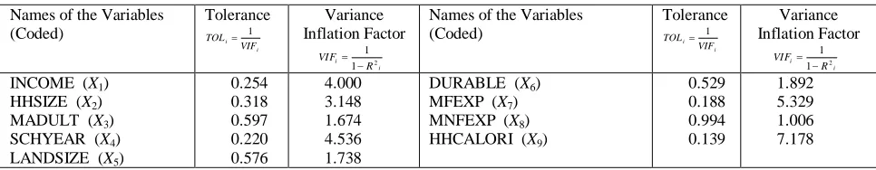
Table 3: Tolerance and Variance Inflation Factors for Different Explanatory Variables

Names of the Variables (Coded)

Tolerance

i i

VIF TOL  1

Variance Inflation Factor i i R VIF ₂ 1 1  

Names of the Variables (Coded)

Tolerance

i i

VIF TOL  1

Variance Inflation Factor i i R VIF ₂ 1 1  

INCOME (X1)

HHSIZE (X2)

MADULT (X3)

SCHYEAR (X4)

LANDSIZE (X5)

0.254 0.318 0.597 0.220 0.576 4.000 3.148 1.674 4.536 1.738

DURABLE (X6)

MFEXP (X7)

MNFEXP (X8)

HHCALORI (X9)

0.529 0.188 0.994 0.139 1.892 5.329 1.006 7.178 2 i

R is the coefficient of determination in the regression of the regressor Xi on the remaining regressors of the model.

From the Table-3, decision on the existence of multicollinearity can also be taken. According to Kleinbaum et al. [13], the variable X7 and X9 are collinear with other or with each other at a higher degree comparing to the other variables.

Consequently their tolerances are also small comparing to the others. The variables X1, X2 and X4 are also collinear to

the other variables but not at a high degree. Thus multicollinearity is containing in the model variables.

Though the variance inflation factors are not showing sufficient information on multicollinearity, as the values are not exceeding a rule of thumb value 10, it can be concluded that, there do exist a moderate multicollinearity. Another approach to detect multicollinearity the Table-4 for eigenvalues, condition index and condition number is also given here.

the last three eigenvalues are small and hence, corresponding condition indices and condition numbers are showing the presence of strong multicollinearity.

Table 4: Multicollinearity Diagnostic Table by Eigenvalues, Condition Index and Condition Number

C. Finding Interval for the Ridge Parameter

There are various procedures for choosing the value for the Ridge parameter



. Whatever the value of this parameter, the mean square error should have to be smaller than the sum of variances of the OLS estimates of the coefficients. The choice of



belongs to the analysts, of course, and a parameter value should be chosen where results show strong evidence that improvements in the estimates are being experienced. These improvements often take the form of evidence that the estimates are more stable or that prediction is improved.

At first, a non-stochastic interval has been taken arbitrarily. Say, it is: (0, 0.1) and the arbitrary increment used here is: 0.001 for the non-stochastic interval. Now, from the methodology as described before, suppose fifty levels (data points) of the X-matrix had been chosen randomly. These levels were stored separately some other where as a new data matrix for the further segments of the analysis. Calculated tr(H)DF for the values of



(using the non-stochastic interval

for fifty randomly chosen data levels) are examined and it is mentionable that, for





0

the value of the DF i.e., 9

) (H_ 

tr . As we had already said that the trace of HAT-matrix i.e., DF will be stabilized for the value of



to be chosen (Tripp [3], [14]), and it is (approximately) 0.006 to go for the ridge regression. We had chosen the value of



, from the DF-trace because, Tripp.[3], [14] had argued that, stabilization of the effective degrees of freedom gives us the clue of stabilization of the coefficients of the regressors and



is allowed to grow until there is a settling in the effective regression degrees of freedom. In the Fig.1 it shows that the effective degrees of freedom is 8 which means it has dropped down from the original degrees of freedom and it was 9. Here it is mentionable that effective degrees of freedom in regression analysis is very important as the property of the HAT-matrix indicates that ‘apart from _2 _the

prediction variance, summed over the locations of the data points, equals the number of model parameters and as close to correct degrees of freedom, prediction at a data point is more correct. If we apply ridge regression on this chosen fifty data levels i.e. the data matrix with which the DF-trace was analyzed, the results of the coefficients for that data set will also show stability where DF-trace was stabilized for the values of



. For all the values of



, where DF-trace stabilized, the estimates of the coefficients also shows stability. Another thing is that, the sign also changes where the values of



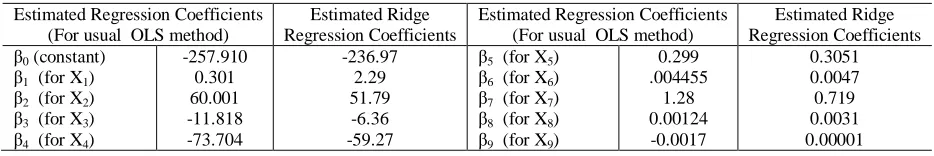
stabilized. Comparing table is showed in the following. Now the ridge estimates for this interval comparing with the OLS estimates are given in the Table-5

Table 5: Comparing Table for OLS Estimates and Ridge Estimates

Estimated Regression Coefficients (For usual OLS method)

Estimated Ridge Regression Coefficients

Estimated Regression Coefficients (For usual OLS method)

Estimated Ridge Regression Coefficients

β0 (constant) β1 (for X1) β2 (for X2) β3 (for X3) β4 (for X4)

-257.910 0.301 60.001 -11.818 -73.704 -236.97 2.29 51.79 -6.36 -59.27

β5 (for X5) β6 (for X6) β7 (for X7) β8 (for X8) β9 (for X9)

0.299 .004455 1.28 0.00124 -0.0017 0.3051 0.0047 0.719 0.0031 0.00001

Let us see what happen if we take another non-stochastic interval. Say, it is (0, 0.2). Here the arbitrary increment is 0.001. Examining all the calculated DF’s for different values of



it shows almost the same situation as we got in the case of the interval (0, 0.1). This is because; the data sets chosen randomly behave in the same manner for any given interval. As it had described before, the stabilization of DF-trace showing for this interval with randomly chosen levels (data points) of the data matrix, the value of the ridge parameter is approximately 0.024 (from a number of estimated values of ridge parameter using statistical programming). For this new arbitrary interval it is apparent that, whatever we choose the length of the non-stochastic interval will not cause any problem to select a value for the ridge parameter.

Let us choose another fifty levels (data points) from the data matrix randomly and again store (save) these levels in some other where and consider them, as a whole, a new set of data matrix. As previously described, for a non-stochastic interval, with an arbitrarily given increment, the trace of the HAT-matrix for different values of



had been examined through statistical programming.

An interesting thing had been revealed from the examined values that, for randomly chosen levels from the original X -matrix, the trace of the HAT-matrix will not give us any clue for the stabilization of the DF. Now the question is-

Eigenvalues ( i ) Condition Number k i i

i , 0,1,2,....,

max _     Condition Index i i    _ max

Eigenvalues ( i ) Condition Number k i i

i , 0,1,2,....,

max _     Condition Index i i    _ max

where to stop for the value of



? At this time we can use the help of generalized cross validation (GCV) procedure (Wahba et al. [2]) which is an another familiar criterion for choosing the value of



. It is mentionable that, GCV is a very well known method from prediction point of view. Thus, here the value for the parameter



, is that point for which GCV is minimum for that particular data matrix (Wahba et al. [2]). Using GCV method, in this case, the value for



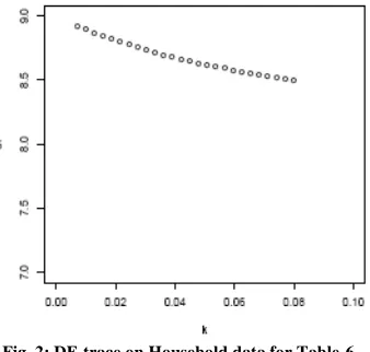
is 0.069.

Fig. 1: DF-trace on Household data for Table-5 _{Fig. 2: DF-trace on Household data for Table-6}

In the same manner fifty levels of the X-matrix had been chosen for one hundred times and for each time a new data matrix had been created. All these data were stored separately. Using all those data matrix one hundred values of



were selected through the same process as described before. It is obvious that, there might come some points or values of



as outliers. To overcome this, 2.5th and 97.5th percentiles (as a rough computation) of those one hundred values of



had been chosen after arranging them in ascending order.

2.5th percentile and 97.5th percentile values had been found 0.007 and 0.08 respectively. Thus our required interval, for the shrinkage parameter of ridge regression, is (0.007, 0.080).

Now again it is needed to see the ridge estimates comparing with the OLS estimates of the coefficients of the explanatory variables as well as the mean square error. Table-6 is showing the ridge estimates for the constructed interval and also the OLS estimates. Here we had used an arbitrary increment (say 0.00292, as we had chosen to have 25 segments of the interval and it is completely arbitrary) for the interval for different values of



. The first and the third column of the table is showing the ordinary least square estimates of the coefficients for different explanatory variables that were used in the model.

Table 6: Comparing Table for OLS Estimates and Ridge Estimates

Estimated Regression Coefficients (For usual OLS method)

Estimated Ridge Regression Coefficients

Estimated Regression Coefficients (For usual OLS method)

Estimated Ridge Regression Coefficients

β0 (constant) β1 (for X1) β2 (for X2) β3 (for X3) β4 (for X4)

-257.910 0.301 60.001 -11.818 -73.704

-251.719 0.2956 53.8893 -11.0105 -48.7849

β5 (for X5) β6 (for X6) β7 (for X7) β8 (for X8) β9 (for X9)

0.299 0.004455

1.28 0.00124 -0.0017

0.3016 0.00443

0.9288 0.00127 0.00004

And the DF-trace for the final interval of the ridge parameter is shown in the Fig.2 which shows less fall of effective degrees of freedom.

At the first point of the examined interval i.e., 0.007, mean square error is,

2 2

ˆ ˆ ˆ _{ˆ ˆ}

( ) [( ) ( )] Ridge squared bias (82.703) 11.3628

2

1( )

k _i

MSE _R E _{R R}

i i



      

 



       

 

While for OLS it was found (130.43683) including mean of error sum of squares. In case of OLS the first term is the coefficient of variances.

Again, at the last point of the interval the mean square error is,

2 2

2 1

ˆ ˆ ˆ _{ˆ ˆ}

( ) [( ) ( )] Ridge squared bias (19.34657) 625.2810

( )

k i

R R R

i i

MSE  E       

 

 

      





While for OLS it was found (1118696.234) including the mean of error sum of squares.

Clearly the ridge regression estimates of the coefficients for the interval, which had been constructed by data levels bootstrapping method, are giving us lower sum of variances of the estimates.

Table-7: Values of



after Slicing the Interval into Twenty Five Segments















0.00700 0.00992 0.01284 0.01576

0.01868 0.02160 0.02452 0.02744

0.03036 0.03328 0.03620 0.03912

0.04204 0.04496 0.04788 0.05080

0.05372 0.05664 0.05956 0.06248

0.06540 0.06832 0.07124 0.07416

0.07708 0.08000

On the other hand, the method of automatic choice for the value of shrinkage parameter, suggested by Hoerl et al. [8] (Procedure was already described in methodology part of this research), gives us the value of



is 0.010109. Obviously it is lying between the interval (0.007, 0.080), and may be the estimates are also started to be stabilized from this point. But one thing has to be focused here that, the change of sign of the coefficient of the 9th variable is negative at the point 0.00992 (Table-8) which is very close to 0.010109. This 9th variable was named as Household Calorie Intake (HHCALORI) and the negative sign of this variable shows incongruity with usual expectancy of sign of its coefficient. Because, in general we know that, household expenditure is highly positively correlated with the expenditure on food and amount of calorie intake is also highly positively correlated with food expenditure. Thus with the constructed interval this important information is coming out that, where the change of sign of the coefficients are happening.

Table-8: OLS Estimates and the Ridge Estimates for the Whole Interval Founded by the Method.

Values of



Constants _β Ridge Estimates

1

(for X1) β2

(for X2) β3

(for X3) β4

(for X4) β5

(for X5) β6

(for X6) β7

(for X7) β8

(for X8) β9

(for X9)

0.00000 -257.910 0.3010 60.0010 -11.8180 -73.7040 0.2990 0.00445 1.2800 0.00124 -0.0017

0.00700 -253.915 0.3006 54.9948 -11.0179 -55.6935 0.2998 0.00446 1.0796 0.00124 -0.0002

0.00992 -252.817 0.2996 54.6920 -11.0129 -49.5892 0.3006 0.00447 0.9347 0.00125 -0.0000

0.01284 -251.719 0.2956 53.8893 -11.0105 -48.7849 0.3016 0.00443 0.9288 0.00127 0.00004

0.01576 -251.681 0.2901 53.0865 -11.0080 -47.9807 0.3029 0.00437 0.9185 0.00127 0.00009

0.01868 -251.220 0.2889 53.0038 -11.0050 -47.7764 0.3036 0.00431 0.9095 0.00129 0.00013

0.02160 -250.825 0.2789 52.8810 -10.9880 -47.5721 0.3044 0.00428 0.8954 0.00129 0.00021

0.02452 -250.428 0.2735 52.7783 -10.8180 -46.8679 0.3048 0.00425 0.8739 0.00130 0.00029

0.02744 -250.180 0.2702 52.5755 -10.8040 -46.6636 0.3055 0.00423 0.8501 0.00130 0.00035

0.03036 -249.932 0.2646 51.7728 -10.7581 -46.4594 0.3089 0.00421 0.7886 0.00131 0.00038

0.03328 -249.734 0.2589 51.9700 -10.7337 -45.9551 0.3116 0.00418 0.7641 0.00131 0.00043

0.03620 -249.636 0.2559 51.4672 -10.6956 -45.9501 0.3175 0.00417 0.7203 0.00133 0.00048

0.03912 -249.438 0.2544 50.7645 -10.6606 -45.8466 0.3219 0.00415 0.6995 0.00134 0.00053

0.04204 -249.340 0.2337 49.9917 -10.6354 -45.7423 0.3225 0.00414 0.6709 0.00136 0.00056

0.04496 -249.142 0.2302 49.9590 -10.5229 -45.6380 0.3233 0.00410 0.6651 0.00138 0.00059

0.04788 -248.974 0.2275 48.4562 -10.5181 -45.5338 0.3239 0.00408 0.6454 0.00139 0.00062

0.05080 -248.856 0.2203 48.5535 -10.4695 -45.3295 0.3251 0.00406 0.6319 0.00139 0.00064

0.05372 -248.948 0.2178 47.9507 -10.4031 -45.1253 0.3295 0.00404 0.6191 0.00141 0.00069

0.05664 -248.751 0.2109 47.4480 -10.3996 -44.9210 0.3327 0.00401 0.5994 0.00142 0.00071

0.05956 -248.653 0.2045 47.1452 -10.3805 -44.8167 0.3336 0.00399 0.5895 0.00142 0.00073

0.06248 -248.255 0.1998 46.9025 -09.3711 -44.7125 0.3347 0.00398 0.5763 0.00144 0.00079

0.06540 -247.957 0.1909 46.5397 -09.3665 -44.7082 0.3361 0.00395 0.5616 0.00145 0.00082

0.06832 -247.859 0.1868 46.1370 -09.3404 -44.6739 0.3383 0.00393 0.5539 0.00145 0.00086

0.07124 -247.761 0.1808 46.0242 -09.2998 -44.3597 0.3392 0.00392 0.5527 0.00145 0.00093

0.07416 -247.683 0.1796 45.9815 -09.2756 -43.8954 0.3404 0.00391 0.5525 0.00145 0.00099

0.07708 -247.625 0.1691 45.8287 -09.2575 -43.6912 0.3417 0.00390 0.5522 0.00146 0.00103

0.08000 -247.598 0.1659 45.8260 -09.2021 -43.6309 0.3431 0.00389 0.5521 0.00146 0.00104

As the GCV (Generalized cross validation) method was also used to choose the value of



for some random samples drawn from the original data, then from prediction point of view it is also important that, if anybody likes to go for the analysis with less error in prediction at different data points, he/she may also get help from the estimated interval of



.

This is a pseudorandom interval because we had given the first interval arbitrarily and the point of stability was also chosen subjectively. A more precise interval may also be obtained by increasing the number of data levels at the stage of random selection of sample. If we draw a histogram (Fig.-3) for the sorted values of the estimated



values (for all five hundred values), we will get that, most of the values are centering in from 0.01 to 0.04.

mean square errors than the ordinary least squares estimates. Thus choice of that parameter, termed as ‘shrinkage parameter’, is a matter of fact that, for what values of it would make us clear to interpret the coefficients of the explanatory variables.

According to Hoerl and Kennard [1], for the value of the shrinkage parameter



, the estimates of the coefficients are stabilized and obviously the mean square error should be less than the sum of the variance of the estimates computed from the OLS method and the proper sign of the coefficients should also be obtained by ridge method.

Fig.-3: Histogram of the Values of Shrinkage Parameters for Constructed Interval

Data used for this analysis, household data, consists of some familiar variables which are correlated to each other more or less. The response variable was Household Expenditure (HHEXP) with some selected explanatory variables– Income (INCOME), Household size (HHSIZE), Number of male adult (MADULT), Years of schooling (SCHYEAR), Size of landholding (LANDSIZE), Durable assets (DURABLE), Monthly food expenditure (MFEXP), Monthly non-food expenditure (MNFEXP) and Monthly household calorie intake (HHCALORI). It is obvious that, monthly non-food expenditure is highly positively correlated with the monthly household calorie intake. Again monthly household expenditure is also positively correlated with the monthly food expenditure, whatever less in amount. And consequently monthly household calorie intake is also positively correlated with HHEXP i.e., monthly household expenditure. But using the ordinary least square procedure the estimated coefficient for the variable HHCALORI is showing negative relation with total household expenditure while total monthly food expenditure is showing positive relation with the response variable. Clearly it is a case of contradictory situation for highly positively correlated two variables which has overcome by the method.

V. CONCLUSION

Another thing is that, as generalized cross validation (GCV) [2] was also used for some number of cases for choosing the value of shrinkage parameter, the interval may also be used, more or less, to take decision from prediction point of view for the value of



. Thus the interval (0.007, 0.080) gives us the information on sign change of the coefficients, stability of the coefficients and also the less error of prediction for different data points of the data set.

ACKNOWLEDGEMENT

The authors would like to convey their enormous gratefulness and sincere gratitude to the respected supervisor, Professor Dr. Pk. M. Motiur Rahman, I.S.R.T., University of Dhaka, for his direct contribution, scholastic guidance, valuable advice, continuous cooperation and endless inspiration throughout the period of the research work. The authors would also like to express their heartfelt eulogies to Professor Dr. Syed Shahadat Hossain, I.S.R.T., University of Dhaka, Professor Dr. M. Shahabuddin, Assistaant Professor Mr. Masum Billah, M. Azizul Hoque, Mohammad Shahid Ullah and Kazi Dawood Hafiz; Lecturer Md. Kamruzzaman and, Malay Kumar Sarkar, Ahsanullah University of Science and Technology, Dhaka, Bangladesh for their encouragements and important suggestions throughout the work.

REFERENCES

[1] A.E. Hoerl, and R.W. Kennard, “Ridge Regression: Biased Estimation for Non-Orthogonal Problems”, Technometrics, vol. 12, pp. 55-67, 1970.

[2] G. Wahba, G.H. Golub, and C.G. Heath, “Generalized Cross Validation as a Method for Choosing a Good Ridge Parameter”, Technometrics, vol. 21, pp. 215-223, 1979.

[3] R.E Tripp, “Non-stochastic Ridge Regression and Effective Rank of the Regressors Matrix”, Virginia Polytechnic Institute and State University, Blacksburg, Virginia, Department of Statistics, 1983.

[4] Kmenta, Jan, “Elements of Econometrics”, The Macmillan Co., 1971.

[5] Damodar N. Gujarati, “Basic Econometrics”, 3rd _{ed., New York: McGraw-Hill, 1995.}

[6] D.A. Belsley, E. Kuh and R.E. Welsch, “Regression Diagnostics, Identifying Influential Data and Sources of Collinearity”, New York: Wiley, 1980.

[7] C. L. Lawson and R. J. Hanson, “Solving Least Squares Problems”, Prentice-Hall, Englewood Cliffs, NJ, 1974.

[8] A.E. Hoerl, R.W. Kennard, and K.F. Baldwin, “Ridge Regression, Some Simulations”, Communications in Statistics, A4, pp. 105-123, 1975.

[9] C.L. Mallows, “Some Comments on

p

C ”, Technometrics, vol. 15, pp. 661-675, 1973.

[10] R.W. Kennard, “A Note on the

p

C -Statistic”, Technometrics, vol. 13, pp. 3-19, 1971.

[11] D. M. Allen, “The Relationship between Variable Selection and Data Augmentation and a Method for Prediction”, Technometrics, vol. 16, pp. 125–127, 1974.

[12] J.T. Robert and Bradley Efron, “An Introduction to the Bootstrap”, New York: Chapman and Hall, 1993

[13] David G. Kleinbaum, Lawrence R. Kupper, and Keith E. Muller, “Applied Regression Analysis and Other Multivariate Methods”, 2nd _ed.,

PWS-Kent, Boston, Mass, 1988.