Application Of Multi-Criteria Decision Making Techniques For Bridge Construction

APPLICATION OF MULTI-CRITERIA

DECISION MAKING TECHNIQUES FOR

BRIDGE CONSTRUCTION

Dr. N. B. Chaphalkar

, Prashant P. Shirke

Associate Professor, Department of Civil Engineering, College of Engineering Pune, India1

M.Tech (C&M) student, Department of Civil Engineering, College of Engineering, Pune2

Abstract: In various stages of project lifecycle, decision making has vital and strategic importance. These decisions are related to different problems and one of the issues is related to selection of alternatives. Decisions made must be independent of any preference or influence. Improper or incorrect selections often increase duration and expenditure of project. The conventional methods for decision making are inadequate for dealing with the imprecise or vague nature of today‟s complex decision problems. To overcome this difficulty, in this paper use of fuzzy Multi-Criteria Decision Making (MCDM) methods is discussed. The aim of this study is to use fuzzy Analytic Hierarchy Process (AHP) and the fuzzy Technique for Order Preference by Similarity to Ideal Solution (TOPSIS) methods for the selection of type of bridge. The proposed methods have been applied to selection of bridge type problem in Pune city. After determining the criteria that affect the selection of type of bridge decisions, fuzzy AHP and fuzzy TOPSIS methods are applied to the problem and results are presented. The similarities and differences of two methods are also discussed.

Keywords:Decision Making, MCDM, Fuzzy Logic, Fuzzy AHP, Fuzzy TOPSIS

I. INTRODUCTION

In India, construction is the second largest economic activity next to agriculture. Construction accounts for nearly 65 per cent of the total investment in infrastructure and is expected to be the biggest beneficiary of the surge in infrastructure investment over the next five years. According to Indo-Italian report, €239.68 billion is likely to be invested in the infrastructure sector over the next five to 10 years; in power, roads, bridges, city infrastructure, ports, airports, telecommunications, which would provide a huge boost to the construction industry as a whole (Indo-Italian Chamber Report, 2008). Decision making is the study of identifying and choosing alternatives based on the values and preferences of decision maker [14]. As magnitude and scope of problem increases, decision making process gets more and more complicated, because with increase in size and scope, number of alternatives and related factors also increase [17]. Good quality highway network is very important for progress of the country and bridges are the vital part of any highway network. Bridges of various types and sizes were built in recent years in India. Defective decision making is one of the major reasons behind losses. (Report of Construction Industry Development Council India, 2006-07) [5]. This paper focuses on the study of new techniques of multi criteria for decision making namely fuzzy AHP and fuzzy TOPSIS for the selection of type of superstructure for bridge construction, where the ratings of various alternatives for the type of structure under various criteria and the weights of all criteria are represented by fuzzy numbers. Further the paper compares outputs given by both methods.

II. MULTI-CRITERIA DECISION MAKING (MCDM)

MCDM constitutes an advanced field of operations research that is devoted to the development and implementation of decision support tools and methodologies to deal with complex decision problems involving multiple criteria, goals, or objectives of conflicting nature. The tools and methodologies provided by MCDM are not just some mathematical models aggregating criteria, points of view, or attributes, but furthermore they are decision-support oriented [17].

consequences of possible actions are not known precisely. These situations imply that a real decision problem is very complicated and thus often seems to be little suited to mathematical modelling because there is no crisp definition. Consequently, the ideal condition for a classic MCDM problem may not be satisfied, in particular when the decision situation involves both fuzzy and crisp data. In general, the term “fuzzy” commonly refers to a situation in which the attribute or goal cannot be defined crisply, due to the absence of well-defined boundaries of the set of observation to which the description applies [15]. Concept of fuzzy logic was introduced in 1965 by Prof. Lofti A. Zadeh, professor of computer science at the University of California in Berkelay. Basically fuzzy logic is a multivalued logic that allows intermediate values to be defined between conventional evaluations like true/false, yes/no etc. and notions like rather tall or very fast can be formulated mathematically in order to apply a more human like way of thinking [16].

III. CASE STUDY

For the application of MCDM techniques a bridge construction project in Pune city is selected. The site location already consists of two existing bridges over the river, but due to increased vehicle population and traffic load resulting into frequent traffic congestions the need for another bridge was necessary. The proposed bridge was to satisfy the following three needs:

 Proposed bridge should solve the problem of traffic congestion in the area along with the elegant aesthetical appearance.

 Service life of existing bridges on site is over and the new bridge has to replace old bridges.

 The site contains old bund on river, recently new spillway gates are constructed for the bund. Proposed bridge should provide an access point for the maintenance of the spillway gates.

Considering needs of the problem and using site data, decision problem is constructed as “Select type of superstructure for proposed bridge”. To solve decision problem, a methodology is prepared using fuzzy AHP and fuzzy TOPSIS methods. These methods require input in the form of verbal judgments from people working in the field. To accomplish the task, a panel of six experts was organized wherein the experts were selected on the basis of their experience in field of bridge construction.

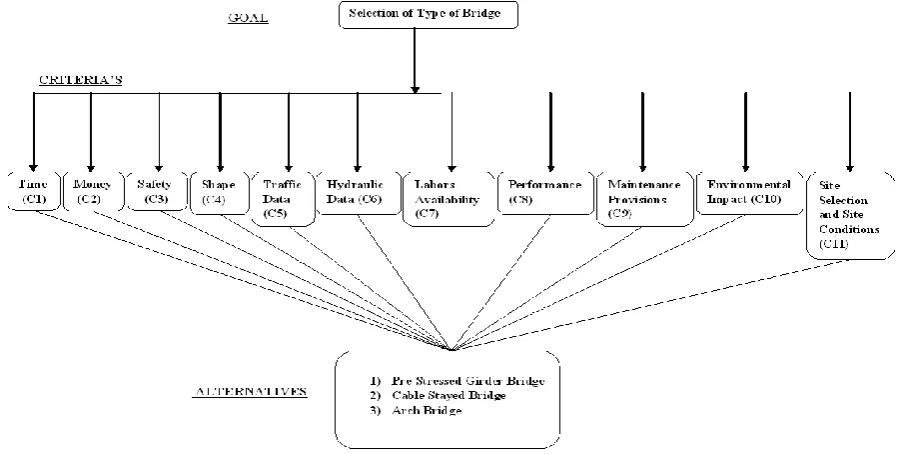
IV. IDENTIFICATION OF CRITERIONS AND DEVELOPMENT OF ALTERNATIVES

First step of the proposed methodology is to identify important criteria affecting the choice of superstructure and develop best possible alternatives for the project. For the identification of criteria Delphi technique is used. Eleven top rated criteria were selected which included time, money, safety, shape, traffic data, hydraulic data, labour availability, performance, maintenance provisions, environmental impact, site selection and site conditions. For the development of alternatives for type of bridge, extensive study of decision problem is required. Local authority had done the study through various consultancies and considered three alternatives regarding type of bridge. For the study the same alternatives are taken under consideration. The three alternatives considered namely Pre-stressed Girder Bridge, Cable Stayed Bridge, and Arch Bridge for the study.

A. Solution by fuzzy AHP

TABLEI: Verbal Judgments

Sr. No Verbal Judgment for Comparing Criteria

Fuzzy Number

Verbal Judgment for Comparing

Alternatives

Fuzzy Number

1 Very Unimportant (VU) ( 0, 0, 2 ) Rejected (R) ( 0, 0, 2 ) 2 Unimportant (U) ( 1, 2, 3 ) Not Preferred (NP) ( 1, 2, 3 )

3 Medium Unimportant

(MU) ( 2, 3.5, 5 )

Slightly non preferable

(SNP) ( 2, 3.5, 5 ) 4 Equally Important (EI) ( 4, 5, 6 ) Equally Preferable (EP) ( 4, 5, 6 ) 5 Medium Important (MI) ( 5, 6.5, 8 ) Slightly Preferred (SP) ( 5, 6.5, 8 ) 6 Important (I) ( 7, 8, 9 ) Preferred (P) ( 7, 8, 9 ) 7 Very Important (VI) ( 8, 10, 10 ) Very Preferred (VP) ( 8, 10, 10 )

Step 1: Construction of hierarchy

The first step of the AHP method is to determine all the important criteria, possible alternatives and define their relationship in the form of a hierarchy as shown in Figure 1. According to [4], fuzzy TOPSIS algorithm is capable of handling only single tier problems, while fuzzy AHP can handle more than one tier problems.

Step 2: Evaluation of fuzzy pair wise comparisons

Questionnaire for fuzzy AHP is prepared keeping in mind type and nature of input required to solve the problem. Questionnaires are filled through direct communication with the panel of experts. Definition of the hierarchical relation is followed by pair wise comparisons of all the criteria on the same level of the hierarchy. The pair wise comparison is performed by using linguistic terms given in Table 1. The fuzzy sets used for this study are taken from [4].

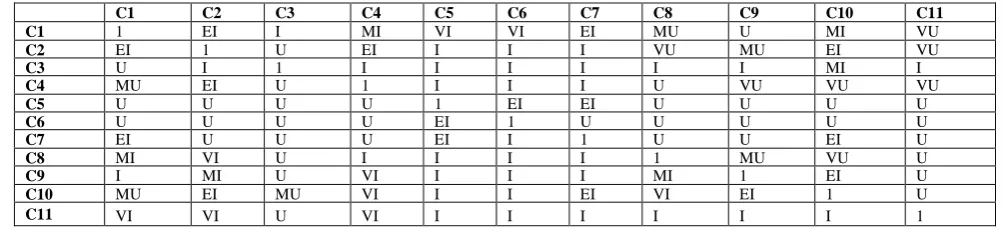
Step 3: Construction of fuzzy decision matrix

After the evaluation of criteria and alternatives using linguistic variables, the fuzzy decision matrix as shown in table 2 is constructed for each of the expert. The values in the upper triangular matrix are filled by using the expert‟s judgments and the lower triangular matrix is filled by using the reverse of the verbal judgements. For e.g. the verbal judgement of comparison between criterion C1 (time) and C3 (safety) is „I‟ (important) in upper triangular matrix whereas in the lower triangular matrix, the reverse verbal judgment is „U‟ (unimportant).





 _n

i i i i

g g W

1

Each verbal judgment in the decision matrix represents a triangular fuzzy set given in Table 1 which is used for further calculations shown in Table 3. To facilitate fuzzy weight calculations, above matrix in Table 2 is further divided in Upper bound matrix (AU), Most likely matrix (AM), Lower bound matrix (AL). Upper bound matrix represents the higher values in the set. For example in the fuzzy set (4, 5, 6) for „Equally Important‟ verbal judgement, the upper bound value is 6, most likely value is 5 and the lower bound value is 4. Table 3 shows the triangular fuzzy set for the first row of the Fuzzy Decision Matrix for First Expert whereas Table 4, 5 and 6 show the first row of each of the upper bound matrix (AU), most likely matrix (AM), lower bound matrix (AL) for first expert.

Table II: Fuzzy decision matrix for first expert

TableIII:Matrix calculation table

C1 C2 C3 C4 C5 C6 C7 C8 C9 C10 C11

Fuzzy decision matrix _{C1 1 (4,5,6) (7,8,9) (5,6.5,8) (8,10,10) (8,10,10) (4,5,6) (2,3.5,5) (1,2,3) (5,6.5,8) (0,0,2)}

Upper bound matrix for first expert _{C1 1 6 9 8 10 10 6 5 3 8 2}

Most likely matrix for first expert _{C1 1 5 8 6.5 10 10 5 3.5 2 6.5 0}

Lower bound matrix for first expert _{C1 1 4 7 5 8 8 4 2 1 5 0}

Step 4: Construction of element weight

Normalization of Geometric Mean Method (NGM) is used to calculate element weights of criteria by using the equation

In the equation,

gi = Geometric mean of criterion i.

rij = Comparison value of criterion i to criterion j. wi = ith criterion weight.

Step 4.1: Calculation of Geometric Mean





ij n

j

i r

g

1

1

  

For Upper Bound Matrix AU, Geometric Mean for Time (C1) criteria from row C1 of Table 4 is calculated as u1 = (1 x 6 x 9 x 8 x10 x 10 x 6 x 5 x 3 x 8 x 2) ^ (1/11) = 5.1113

The Geometric Mean of other criteria calculated in upper bound matrix, are summarized in Table 3.

Step 4.2: Calculation of element weight

Using NGM, element weight for Time criterion is calculated as 0.0981. Similarly the element weights are calculated for other criteria in upper bound matrix, most likely matrix and lower bound matrix from first expert‟s decision matrix which are summarized in Table 4.

C1 C2 C3 C4 C5 C6 C7 C8 C9 C10 C11

C1 1 EI I MI VI VI EI MU U MI VU

C2 EI 1 U EI I I I VU MU EI VU

C3 U I 1 I I I I I I MI I

C4 MU EI U 1 I I I U VU VU VU

C5 U U U U 1 EI EI U U U U

C6 U U U U EI 1 U U U U U

C7 EI U U U EI I 1 U U EI U

C8 MI VI U I I I I 1 MU VU U

C9 I MI U VI I I I MI 1 EI U

C10 MU EI MU VI I I EI VI EI 1 U

TableIV:Weight calculation table

Step 4.3: Identify minimum, mean and maximum element weight

After the calculation of the element weight, minimum, mean and maximum element weight from Table 4 for each of the criteria is identified. E.g. Minimum, mean and maximum element weight for Time (C1) are (0.0981, 0.0981, 0.0996). Similarly steps 3 and 4 are repeated for other experts.

Step 5: Aggregation of Experts Decision

As the responses are obtained from six experts they are aggregated into one by using the centre of sum method. Equation of centre of sum method is represented as

 





mC Where, Z* represents the aggregated value

For Time (C1) criteria, aggregated value is calculated as 0.0805 by using above equation. The calculated aggregated weights of other criteria are summarized in Table 5. These results show that „Performance of particular type of bridge (C8)‟ is most dominating criteria in the selection process followed by „site selection and site conditions‟. Steps 3 to 5 are followed for calculating aggregated weights of all alternatives with respect to all criteria. The results are summarized in Table 5:

TableV: Aggregated and overall weights of all alternatives

Aggregated weights Overall weights

A1 A2 A3 A1 A2 A3

C1 0.4921 0.1672 0.3064 C1 0.0396 0.0135 0.0247

C2 0.4813 0.1747 0.3102 C2 0.0404 0.0147 0.0261

C3 0.4429 0.1831 0.4038 C3 0.0492 0.0203 0.0449

C4 0.2237 0.4976 0.3266 C4 0.0120 0.0267 0.0175

C5 0.5007 0.2023 0.2480 C5 0.0376 0.0152 0.0186

C6 0.5707 0.1423 0.2868 C6 0.0650 0.0162 0.0327

C7 0.4896 0.2230 0.3288 C7 0.0351 0.0160 0.0235

C8 0.4826 0.2009 0.3493 C8 0.0796 0.0331 0.0576

C9 0.4739 0.1887 0.4253 C9 0.0414 0.0165 0.0372

C10 0.3803 0.2231 0.4934 C10 0.0410 0.0241 0.0532

C11 0.6592 0.1937 0.2799 C11 0.0809 0.0238 0.0343

Final Weight 4.6263 2.3966 3.7585

Step 6: Calculation of Overall Weight of each alternative

Now overall weight of each alternative is calculated by multiplying weight of main criteria with local weight of criteria from Table 5 for each alternative.

Example: For Time criterion and Pre-Stressed Girder Bridge alternative Weight for Time criterion: 0.0805

Weight of Pre-Stressed Girder Bridge concerning Time criterion: 0.4921

Overall weight of Pre-Stressed Girder Bridge for Time criterion: 0.0805 x 0.4921 = 0.0396. To calculate final weights for each alternative, each alternative weights of all criteria are added.

Criteria Geometric mean values for upper bound matrix of first expert

Upper bound matrix

weights

Most likely matrix

weights

Lower bound

matrix weights

Aggregated weights of criteria for first expert

C1 5.1113 0.0981 0.0981 0.0996 0.0805

C2 4.3065 0.0826 0.0776 0.0823 0.0840

C3 6.5989 0.1266 0.1362 0.1484 0.1111

C4 3.6591 0.0702 0.0617 0.0640 0.0537

C5 2.9680 0.0569 0.0495 0.0401 0.0751

C6 2.7868 0.0535 0.0456 0.0353 0.1139

C7 3.6243 0.0695 0.0650 0.0542 0.0716

C8 4.9850 0.0956 0.0941 0.0941 0.1649

C9 5.7490 0.1103 0.1152 0.1160 0.0874

C10 5.4702 0.1049 0.1094 0.1072 0.1078

Final weight of alternative A1- Pre-Stressed Girder Bridge (4.6263) is maximum, followed by A3- Arch Bridge (3.7585) and then A2-Cable Stayed Bridge (2.3966). According to final weights „Pre-Stressed Girder Bridge‟ is most favourable alternative for the project.

B. Solution by fuzzy TOPSIS

The TOPSIS method was firstly proposed by [21]. The basic concept of this method is that the chosen alternative should have the shortest distance from the positive ideal solution and the farthest distance from negative ideal solution. Positive ideal solution is a solution that maximizes the benefit criteria and minimizes cost criteria, whereas the negative ideal solution maximizes the cost criteria and minimizes the benefit criteria [4]. In this paper fuzzy TOPSIS method is also proposed for the selection problem of type of bridge. Initially, the six decision-makers evaluated the importance of criteria by using the linguistic variables in Table 6. The stepwise analysis of fuzzy TOPSIS algorithm with the help of the case study is explained in the following sections.

Step 1: Evaluation of criteria

After the identification of criteria and development of alternatives, evaluation of criteria and alternatives is done by the selected panel of experts. Experts are asked to give opinions in the form of verbal judgments. Based on the type of evaluation, verbal judgments are developed for the study. Fuzzy sets used here are taken from [4]. Verbal judgments from different experts are going to be used as an input for the TOPSIS algorithm. Questioners are filled from them through direct communication with them.

TableVI: Linguistic judgments

Sr No

Verbal judgment for

weight of criteria Fuzzy number

Verbal judgment for rating of

alternative Fuzzy number

1 Very Low (VL) ( 0, 0, 0.2 ) Rejected (R) ( 0, 0, 2 ) 2 Low (L) ( 0.1, 0.2, 0.3 ) Not Preferred (NP) ( 1, 2, 3 ) 3 Medium Low (ML) ( 0.2, 0.35, 0.5 ) Slightly Non Preferable (SNP) ( 2, 3.5, 5 ) 4 Medium (M) ( 0.4, 0.5, 0.6 ) Equally Preferable (EP) ( 4, 5, 6 ) 5 Medium High (MH) ( 0.5, 0.65, 0.8 ) Slightly Preferred (SP) ( 5, 6.5, 8 ) 6 High (H) ( 0.7, 0.8, 0.9 ) Preferred (P) ( 7, 8, 9 ) 7 Very High (VH) ( 0.8, 1, 1 ) Very Preferred (VP) ( 8, 10, 10 )

Step 2: Aggregation of weights

Group evaluation is made by aggregating each expert‟s opinion into one. For fuzzy TOPSIS weights and ratings given by expert panel are aggregated by using Max-Min method by following formula

} { ,

1 },

{ _max

min

1

k k K

k k k

k

c c

b K b a

a   

 Here,

a= minimum value in the set b= mean value in the set c= maximum value in the set k = no. of experts

Aggregated weights and ratings are shown in Table 7. Example: For Criteria Time (C1)

TABLEVII: Weights of time criteria from six experts

Sr

No Criteria

Expert

E1 E2 E3 E4 E5 E6

1 Time (C1) 0.7, 0.8, 0.9 0.5, 0.65, 0.8 0.8, 1, 1 0.5, 0.65, 0.8 0.4, 0.5, 0.6 0.5, 0.65, 0.8

Aggregation of weights of criteria by Max-Min method In this case:

a = 0.4 ; _



1

b = 0.7083 ; c = 1

Step 3: Construct the fuzzy decision matrix

Aggregation of weights for all criteria is completed by following same procedure described in step 2 and results are given under „Weight‟ column of Table 8. Aggregation of ratings of all alternative A1, A2 and A3 are obtained for each criterion by following same procedure described in step 2 and results and are given under column A1, A2 and A3 of Table 8.

Step 4: Construct the fuzzy normalized decision matrix

Construction of fuzzy decision matrix is followed by normalization of ratings.

For fuzzy TOPSIS algorithm the linear scale transformation is used for the process of normalization wherein every element in each row is divided by highest element in the row. In the normalization by linear scale transformation, every element in each row is divided by highest element in the row. For example for row C1 in table highest value is „10‟, so every rating of each alternative is divided by „10‟. Normalized ratings of all alternatives are shown in Table 9 which represents the fuzzy normalized decision matrix.

TABLEVIII: Fuzzy decision matrix

A1 A2 A3 Weight

C1 7, 9.3333, 10 1, 4.75, 9 5,7.5,9 0.4,0.7083,1 C2 8, 10, 10 0,3.3333,9 0,5.1667,9 0.5,0.8417,1 C3 1, 7.4167, 10 1,5.25,9 5,7.9167,10 0.5,0.8083,1 C4 1, 4.5, 8 7,8.6667,10 5,8.4167,10 0.2,0.6833,1 C5 7, 8, 9 7,8,9 7,8,9 0.4,0.75,0.9 C6 7, 8, 9 5,7.75,9 7,8,9 0.4,0.7667,1 C7 7, 8,6667, 10 2.6.25,9 5,7.75,9 0.1,0.6083,1 C8 7, 8, 9 1,7.3333,10 7,8.6667,10 0.5,0.8750,1 C9 7,9,10 1,5.75,9 2,7.25,9 0.4,0.8167,1 C10 7,8.6667,10 1,6,9 0,6.6667,9 0.5,0.8417,1 C11 7,8.6667,10 2,7.5833,10 7,8.3333,10 0.5,0.7833,1

TABLEIX: Fuzzy normalized decision matrix

A1 A2 A3 Weight

C1 0.7,0.9333,1 0.1,0.4750,0.9 0.5,0.75,0.9 0.4,0.71,1 C2 0.8,1,1 0,0.3333,0.9 0,0.5167,0.9 0.5,0.84,1 C3 0.1,0.7417,1 0.1,0.52,0.9 0.5,0.7917,1 0.5,0.81,1 C4 0.1,0.45,0.8 0.7,0.8667,1 0.5,0.8417,1 0.2,0.68,1 C5 0.78,0.89,1 0.78,0.89,1 0.78,0.89,1 0.4,0.75,0.9 C6 0.78,0.89,1 0.56,0.86,1 0.78,0.89,1 0.4,0.77,1 C7 0.7,0.8667,1 0.2,0.62,0.9 0.5,0.77,0.9 0.1,0.61,1 C8 0.7,0.8,0.9 0.1,0.7333,1 0.7,0.8667,1 0.5,0.88,1 C9 0.7,0.9,1 0.1,0.57,0.9 0.2,0.72,0.9 0.4,0.82,1 C10 0.7,0.8667,1 0.1,0.6,0.9 0,0.6667,0.9 0.5,0.84,1 C11 0.7,0.8667,1 0.2,0.7583,1 0.7,0.8333,1 0.5,0.78,1

Step 5: Construct the fuzzy weighted normalized decision matrix

After formation of fuzzy normalized decision matrix ratings of alternatives and weights of criteria are combined to construct fuzzy weighted normalized decision matrix. To construct this matrix each set of rating is multiplied by set of weight in same row.

For example for row C1 and for alternative A1 in Table 9 (0.7, 0.9333, 1) x (0.4, 0.71, 1) = (0.28, 0.6626, 1) { 0.7 x 0.4 = 0.28

Step 6: Determining FPIS and FNIS

After the formation of decision matrix Fuzzy positive ideal solution (FPIS) values and Fuzzy negative ideal solution (FPNS) values are developed which are the two extreme values on the scale of our judgment. FPIS values are found out by developing set of highest element in each row. For example for row C1 in Table 10, highest element in all set is „1‟, so FPIS set for criteria C1 is (1,1,1), as shown below. FPNS values are found out by developing set of lowest element in each row from table 10. By following same procedure FPIS and FPNS sets for all criteria‟s are developed.

TABLEX: Weighted normalized decision matrix

A1 A2 A3

C1 0.28,0.6626,1 0.04,0.3373,0.9 0.2,0.53,0.6 C2 0.40,0.84,1 0,0.28,0.9 0,0.4340,0.9 C3 0.05,0.6008,1 0.05,0.42,0.9 0.25,0.6413,1 C4 0.02,0.31,0.8 0.14,0.5894,1 0.1,0.5724,1 C5 0.31,0.67,0.9 0.31,0.67,0.9 0.31,0.67,0.9 C6 0.31,0.69,1 0.22,0.66,1 0.31,0.69,1 C7 0.07,0.5287,1 0.02,0.38,0.9 0.05,0.47,0.9 C8 0.35,0.70,0.90 0.05,0.6453,1 0.35,0.7627,1 C9 0.28,0.74,1 0.04,0.47,0.9 0.08,0.59,0.9 C10 0.35,0.7280,1 0.05,0.50,0.9 0,0.56,0.9 C11 0.35,0.6760,1 0.10,0.5915,1 0.35,0.65,1

FPIS d* {(1,1,1) (1,1,1) (1,1,1) (1,1,1) (0.9,0.9,0.9) (1,1,1) (1,1,1) (1,1,1) (1,1,1) (1,1,1) (1,1,1)}

FPNS d- {(0.04,0.04,0.04) (0,0,0) (0.05,0.05,0.05) (0.02,0.02,0.02) (0.31,0.31,0.31) (0.22,0.22,0.22) (0.02,0.02,0.02) (0.05,0.05,0.05) (0.04,0.04,0.04) (0,0,0) (0.10,0.10,0.10)}

After developing the FPIS and FPNS for the scale of judgment, the distance of each alternative from FPIS (d*) and FPNS (d-) is found out by vertex method as shown below.

] ) ( ) (

) [( 3 1 ) ,

( 2

2 1 2 2 1 2 2

1 l m m n n

l n

m

dv       



Where, l1, m1, u1 = Values from FPIS and FPNS set for particular row l2, m2, u2 = Corresponding values from Table 10 for particular row

After calculating distance of each alternative from d* and d-, total weight of each alternative is calculated. Total weight of each alternatives with respect to FPIS (d*) and total weight of each alternatives with respect to FPNS (d-) is to be calculated by adding all distances for each alternative.

Step 10: Determining Closeness Coefficient (CC)

A closeness coefficient (CCi) is defined to rank all possible alternatives which represents the distance of particular alternative to the fuzzy positive ideal solution (A*) and fuzzy negative ideal solution (A-) simultaneously. Higher closeness coefficient represents particular alternative is closer to FPIS and away from FPNS. The closeness coefficient of each alternative is calculated as

)

(_{d d}*

d

CCi _



The closeness coefficients for the alternatives are given in Table 11.

TABLEXI: Total weights of alternatives

Alternative A1 A2 A3

d* _{5.2833 6.5081 5.8162}

d- _{6.8869 6.1154 6.4108}

Step 11: Ranking of Alternatives

According to the closeness coefficients in Table 11 for three alternatives, the ranking order of three alternatives is determined as A1 >A3 > A2 i.e. pre-stressed girder bridge, arch bridge, cable stayed bridge. The first alternative is closer to the FPIS and farther from the FNIS. According to the results „pre-stressed girder bridge‟ is the most favourable alternative for the project.

V OBSERVATIONS & CONCLUSIONS

From the study, it was found that both methods suggested pre-stressed girder bridge as the first alternative with highest final weight with fuzzy AHP and highest closeness coefficient with fuzzy TOPSIS. Second alternative given by these methods is arch bridge and cable stayed bridge as the third alternative (Table 12).

TABLEXII: Comparison of results of Fuzzy AHP and Fuzzy TOPSIS

Type of Bridge _{Fuzzy AHP Fuzzy TOPSIS}

Final weight Closeness coefficient

Pre-stressed Girder Bridge 4.6263 0.5659 Arch Bridge 3.7585 0.5343 Cable Stayed Bridge 2.3966 0.4844

During the analysis it is found that both methods have some advantages and limitations for the problem which are summarized below.

 In terms of calculation, fuzzy AHP requires more complex calculations then fuzzy TOPSIS.

 Fuzzy AHP uses pair wise computations for the evaluation of problem, whereas no pair wise computations is used in fuzzy TOPSIS.

 In fuzzy AHP framework as the number of criteria increases, the pair wise comparisons become more cumbersome to handle and there is increased risk of inconsistency generation.

 In fuzzy AHP output, final weights of criteria and alternatives can be equal or zero and this condition is not practically acceptable.

 In the fuzzy AHP, in some cases if two criterions are of different nature, then it gets difficult to make comparison between them e.g. it is difficult to compare criteria like safety and environmental impact.

 In fuzzy AHP, difficulty may arise while comparing alternatives, if concerning criteria is does not have direct impact on decision problem.

In Indian scenario, use of these advanced techniques along with the conventional methods will be capable of handling complex decision problems and enhance the decision making process.

REFERENCES

[1] Thomas, L., Saaty. (2008). Decision making with the analytic hierarchy process. International Journal of Services Sciences, 1(1), 83-98. [2] Aviad, S., Marat, G.. (2005). AHP-Based Equipment Selection Model for Construction Projects. Journal of construction engineering and

management, ASCE, 131 (12), 1263–1273.

[3] Aşkın ÖZDAĞOĞLU, Güzin ÖZDAĞOĞLU. (2007). Comparison of AHP and fuzzy AHP for the Multi-Criteria Decision Making processes with linguistic evaluations. 65-85.

[4] Irfan, Ertugrul & Nilsen, Karakasoglu. (2007). Comparison of fuzzy AHP and Fuzzy TOPSIS methods for facility location selection. International Journal of Advanced Manufacturing Technology, 39, 783–795.

[5] Nang – FeiPan, (2008). Fuzzy AHP approach for selecting the suitable bridge. Automation in construction, 17, 958–965.

[6] Amin, Kaboli, M.B., Aryanezhad, Kamran, Shahanaghi and Iman, Niroomand. (2007). A New Method for Plant Location Selection Problem: A Fuzzy-AHP Approach, International Journal of Human and Social Sciences, 1-4244-0991-8, 586-582

[7] Chen, C. T., (2000). Extensions of the TOPSIS for group decision-making under fuzzy environment. Fuzzy sets and Systems, 114, 1-9.

[8] Hsu-Shih, Shiha, Huan-JyhShyurb, Stanley Lee. (2007). An extension of TOPSIS for group decision making. Mathematical and Computer Modelling, 45, 801–813.

[10] Zhongliang, Yue,. (2010). An extended TOPSIS for determining weights of decision makers with interval numbers. Knowledge-Based Systems, 24, 146–153.

[11] Mahmoodzadeh, S., Shahrabi, J., Pariazar, M., and Zaeri, M. S. (2007). Project Selection by Using Fuzzy AHP and TOPSIS Technique. International Journal of Human and Social Sciences, 1(3), 135-140.

[12] Ming-Chyuan Lin a, Chen-Cheng Wang a, Ming-Shi Chen a, C. Alec Chang, (2008). Using AHP and TOPSIS approaches in customer-driven product design process. Computers in industry, 59, 17–31.

[13] Yu-JieWanga, Hsuan-Shih Lee, (2007). Generalizing TOPSIS for fuzzy multiple-criteria group decision-making. International Journal of Computers and Mathematics with Applications, 53, 1762–1772.

[14] Harris (2009), „Introduction to decision making”, Online Available, 2011.

[15] Bellman, Zadeh (1970), “Decision making in fuzzy environment”, Management Science, 17B: 141-B164. [16] L. A. Zadeh (1965), “Fuzzy Sets”, Information and Control 8, 338-353.

[17] Von, V., (2003). A fuzzy multi-attribute decision making approach for the identification of the key sectors of an economy: The case of Indonesia. Dissertation Report for Master of Science.

[18] Sam Salem, Richard Miller, (2006). Accelerated Construction Decision‐ Making Process for Bridges. Midwest Regional University Transportation Centre Project.

[19] Cengiz Kaharaman, (2008). Fuzzy Multi-Criteria Decision Making – Theory and Applications with recent developments, Springer publications, New York, USA.

[20] Ross, Timothy J. (2004), Fuzzy Logic with Engineering Applications, John Wiley & Sons Ltd, England.