Sparse Learning in Multiclass Problems.

(1)

ABSTRACT

LI, NAN. Sparse Learning in Multiclass Problems. (Under the direction of Dr. Hao Helen Zhang.)

Multi-category classification is an important topic in statistical learning and data min-ing. It has many applications, such as handwritten zip code digit recognition and cancer type DNA microarray classification. Multi-classification in many practical problems is even more challenging by the presence of a large number of candidate predictors. Espe-cially in biological or medical applications such as microarrays, the overwhelming number of variables far exceeds the size of training samples even though and the underlying model may be sparse. In these applications it is essential to identify important variables for achieving classifiers with higher prediction accuracy and better model interpretability.

(2)

Sparse Learning in Multiclass Problems

by Nan Li

A dissertation submitted to the Graduate Faculty of North Carolina State University

in partial fulfillment of the requirements for the Degree of

Doctor of Philosophy

Statistics

Raleigh, North Carolina 2011

APPROVED BY:

Dr. Howard Bondell Dr. Dennis Boos

Dr. Yichao Wu Dr. Hao Helen Zhang

(3)

DEDICATION

(4)

ACKNOWLEDGEMENTS

I would like to express sincerest gratitude to my advisor Dr. Hao Helen Zhang for her constant guidance, encouragement and support, both intellectually and financially, in my PhD study. Without her, this would never have come true. During these years, it has been such a great pleasure and honor to have the opportunity to study with her and learn from her. I will always be very thankful for her wisdom, knowledge, and patient.

I also thank Dr. Dennis Boos, Dr. Howard Bondell and Dr. Yichao Wu for being my committee members, reviewing my dissertation, providing constructive comments and offering great graduate lectures. And I greatly appreciate Dr. Jacqueline Hughes-Oliver recruiting me to the Statistics Department and offering me the invaluable opportunity to continue on my Ph.D study. I would like to thank her for her guidance, support and consideration.

Special thanks to my good friends, Dongxia, Yin zheng, Chao jingyi and Liping, for seeing me laughers and tears and sharing the ups and downs along this way.

(5)

LIST OF TABLES

Table 3.1 Simulation results for the four-class linear example 1. . . 42

Table 3.2 Simulation results for four-class linear example 2. . . 43

Table 3.3 Simulation results for the five-class linear example. . . 43

Table 3.4 Simulation results for the four-class linear example 3. . . 44

Table 3.6 Classification and variable selection results for the nonlinear example 46 Table 3.7 Class distribution of the Leukemia data . . . 49

Table 3.8 Classification and variable selection results for the Leukemia data 50 Table 3.9 Class distribution of the SRBCT data . . . 50

Table 3.10 Classification and variable selection results for the SRBCT data . 51 Table 4.1 Simulation results for the four-class linear example 1 . . . 58

Table 4.2 Simulation results for four-class example 2 . . . 60

Table 4.3 Simulation results for the four-class example 3 . . . 61

Table 4.5 Simulation results for nonlinear example . . . 63

Table 4.6 Class distribution of the Leukemia data . . . 65

(8)

LIST OF FIGURES

Figure 1.1 Optimum hyperplane for binary classification in separable case. Reprinted

from Hastie et al. (2001) . . . 6

Figure 1.2 SVM for separate case . . . 7

Figure 1.3 SVM for Non-separate Case . . . 11

Figure 2.1 SCAD penalty with a=3.7 and λ= 1 . . . 22

Figure 3.1 The Bayes boundary for the four-class example. . . 41

Figure 3.2 The Bayes boundary for the nonlinear three-class example. . . 47

Figure 4.1 The Bayes boundary for the four-class example 1. . . 59

(9)

Chapter 1 Review for Classification Problems

1.1 The Bayes Classifier

In a typical classification problem, we are given a training data set containing n pairs of observations {(x1, y1),(x2, y2), . . . ,(xn, yn)}, where xi = (xi1, . . . , xid)T ∈Rd is the input vector, and the output yi ∈ A = {1,2, . . . , K} indicates its class label. Our task is to learn a discriminating rule φ :Rd _{→ {}₁_,₂_{, . . . , K}_} _{so that when given a new input}_x _we can accordingly assign it a class label fromA.

Let us have a look at three classification examples in the real world. First is the email/spam data from Hastie, Tibshirani & Friedman (2001). Emails provide a fast and economical way of communication, as well as result in a dramatic increase of spam emails. In this 4601 email message dataset, we want to find an efficient spam/email filtering method which predicts whether a message is a true email or a spam. The input are the relative frequencies of 57 most commonly occurring words and punctuation marks in the email messages. The output is the email type (email/spam).

The second example is the handwritten zip code digit recognition data, which is also from Hastie et al. (2001). In this dataset, handwritten ZIP codes on envelopes consist of five digits from {0,1, . . . ,9}. Each digit is scanned in image and converted into a 16×16 pixel matrix with each pixel ranging in intensity from 0 to 255. The US postal service wishes to use these pixel mapping as an input, design a system to read handwritten zip codes on mail and output a digit prediction between 0 and 9. This problem has a 256 dimensional input space, x ∈ R256, and the output is one of 10 possible outcomes,

(10)

The last one is cancer classification using DNA microarray data. With the break-through of microarray techniques in biology, expression levels of thousands of genes can be measured simultaneously from a single cell sample. This generates a large amount of high-throughput data with “high dimensional low sample size” property. Given a set of labeled samples from different cancer types, our goal is to predict the diagnostic cancer category of a sample on the basis of its gene expression profile. Molecular di-agnosis based on high-throughput genomic data present a major challenge due to the overwhelming number of variables and complex multi-class nature of cancer samples. In this so called “large p small n” case, most classical classification methodologies, like Fisher linear discriminant analysis (LDA), quadratic discriminant analysis (QDA) and logistic regression, cannot be applied since the smaller number of samples does not pro-vide enough information to estimate the underlying high-dimensional covariance matrix. The key reason for this failure is that among p columns of microarray data many are highly correlated, thus carrying redundant information. Therefore the covariance matrix is singular and cannot be inverted. To confront this challenge, some modern solutions have been developed, including a family of regularization methods, K-nearest neighbor (K-NN), and SVM.

In general statistical framework, we assume (xi, yi) arei.i.d.from an unknown prob-ability distributionP(x, y). Given a classifierφ, its performance is usually measured by the misclassification error rate i.e. the probability that the classification is different from

y,

GE(φ) = P(y6=φ(x)) =E(x,y)[I(y6=φ(x))]. (1.1)

The optimal classifier in terms of minimizing this misclassification error rate is known as Bayes classifier.

Let pk(x) = P(y = k|x) be the conditional probability of class k given x for k = 1, . . . , K. The Bayes classifier which minimizes GE is then given by

φB(x) = arg min

(11)

vector ˆf ={fˆ1, . . . ,fˆK} and define the decision rule as ˆ

φ(x) = arg max

1≤k≤K ˆ

fk(x). (1.3)

Each ˆfk represents the strength of the evidence that an example with inputxbelongs to the class k, k = 1,2, . . . , K. A classifier induced by ˆf assigns an example with x to the class with the largest ˆfk(x).

There are mainly two types of classification methods, soft classification and hard classification. Soft classification approximates the Bayes rule by estimating ˆpk(x) first and then classifying to the maximum estimated probability. Among them are logistic regression, LDA, and QDA. On the other hand, hard classification bypasses the posterior probability ˆpk(x) and directly estimating the argmax function in (1.3). A famous example is support vector machine (SVM) (Vapnik (1995)).

In the rest of this Chapter, we will give a brief review of these methods.

1.2 Linear Discriminant Analysis (LDA) and Quadratic

Discriminant Analysis (QDA)

LDA and QDA are developed under normal distribution assumptions for explanatory variables. Let gk(x) denote the density of class k, and πk denote the prior probability of class k, with PK

k=1πk = 1. Then the posterior distribution of class k after observing x is:

pk(x) = gk(x)πk

PK

k=1gk(x)πk

, k = 1, . . . , K.

Now assume the distribution for classk is multivariate normal with meanµ_k and covari-ance matrix Σk,

gk(x) =

1 (2π)d/2_|_Σ

k|1/2

exp[−1

2(x−µk) T_Σ−1

(12)

Then the Bayes classification is to the class with maximum

Dk = log[gk(x)πk] = loggk(x) + logπk =−1

2(x−µk)Σ

−1

k (x−µk) T ₋ 1

2log|Σk|+ logπk.

In practise, the parameters of the multivariate normal distributions are not known. Using training data, we can estimate them by

• πˆk =nk/n, where nk is the number of observations in class k,

• µˆ_k=P

yi=kxi/nk,

• Σˆk =P_y_i=_k(xi−µˆk)(xi−µˆk)T/(nk−1),

• Σˆ =PK

k=1 P

yi=k(xi−µˆk)(xi−µˆk)T/(n−K).

Then we produce an estimate for Dk and classify to the class with highest estimated ˆ

Dk. The boundary between two classes is a quadratic function of x, so this method of classification is known as QDA.

Further suppose that all the classes have a common covariance matrix Σ. Then all the classification boundaries among the K classes are linear functions of x and we can maximize

Dk=xΣ−1µTk −µkΣ

−1

µT_k/2 + logπk. This procedure is known as LDA.

1.3 Logistic Regression

Logistic regression assumes the following forms of log-odds (McCullagh and Nelder 1989):

log P(y=k|x)

P(y=K|x) =βk0+β T

(13)

Those are linear functions in the explanatory variables, so are the decision boundaries. Inverting the log-odds, we have the posterior probabilities as:

P(y =k|x) = exp(βk0+β T kx) 1 +PK−1

l=1 exp(βl0+β

T l x)

, k= 1, ..., K −1,

P(y=K|x) = 1

1 +PK−1

l=1 exp(βl0+β

T l x)

.

(1.4)

They automatically sum to one and remain in (0,1). Logistic regression models are usually fit by maximizing the conditional likelihood of ygiven xusing the training data, like binomial or multinomial log-likelihood.

In logistic regression, only the conditional distribution P(y =k|x) are specified and the marginal density of x are left arbitrarily as any density function P(x). While in LDA and QDA, the joint distribution of x and y with P(x) is specified a mixture of Gaussian. Therefore logistic regression is more general and should be more robust. But if the Gaussian assumption made by LDA/QDA is appropriate, then LDA/QDA tend to estimate the parameters more efficiently by using more information from the data (Hastie et al. (2001)).

1.4 Support Vector Machine

1.4.1 Binary SVM

(14)

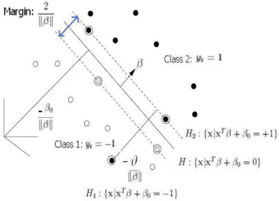
from original input space to a higher dimensional feature space and then constructing a higher dimensional hyperplane that optimally separates the data into two categories. Lin (2002) showed that under some general conditions, the SVM solution approaches Bayes rule when the sample size increases.

Figure 1.1: Optimum hyperplane for binary classification in separable case. Reprinted from Hastie et al. (2001)

We will start with the simplest case: linear machines trained on separable data. Recall that the training data consist of n pairs of {xi, yi}, i = 1, ..., n,with x ∈ Rd. In binary classification, we usually haveyi ∈ {−1,1}. There exists a hyperplane completely separating the two classes. Define the hyperplane as {x:f(x) = xT_β₊_β

0 = 0}, where β is the normal to this hyperplane, |β0|/||β|| is the perpendicular distance from the

hyperplane to the origin, and ||β|| is the Euclidean norm of β. The SVM looks for the optimal hyperplane as:

max β0,β,||β||2=1

M

subject to yi(xTi β+β0)≥M,fori= 1, ..., n.

(15)

Rescalingβandβ0, we can get rid of||β||= 1 by replacing the constraint condition with

yi(xT_i β+β0)≥M||β||. (1.6)

If arbitrarily set ||β|| equal to 1/M, then (1.6) can be written as

yi(xTi β+β0)≥1. (1.7)

The points for which the inequalities (1.7) hold are shown in Figure 1.2.

Figure 1.2: SVM for separate case

Hyperplanes H1 and H2 are parallel and no training data fall between them. Points

on the hyperplane H1 satisfy {x : xTβ+β0 = −1} and points on the hyperplane H2

satisfy {x : xT_β₊_β

(16)

to H1 and | −1−β0|/||β|| from origin to H2, and the margin is 2/||β||. Thus we can

find the hyperplane which gives the maximum margin by minimizing ||β||2_{, subject to}

constraint (1.7). Then (1.5) is equivalent to

min β0,β

1 2kβk

2

subject to yi(xTi β+β0)≥1,for i= 1, ..., n.

(1.8)

This convex optimization problem can be solved by quadratic programming technique. The primal function is obtained by introducing Lagrange multipliers αi ≥0i= 1, . . . , n, one for each of the inequality constraints in (1.8),

LP = 1 2||β||

2₋

n

X

i=1

αi[yi(xTi β+β0)−1]. (1.9)

LP has to be minimized with respect to the primal variables (β0,β) and maximized with

respect to the dual variables αi’s. Setting the first derivatives to zero, we have:

∂LP

∂β0 = 0 =⇒

n

X

i=1

αiyi = 0,

∂LP

∂β = 0 =⇒

n

X

i=1

αiyixi =β.

(1.10)

Substituting β0 and β in (1.9) with (1.10), we get the following Wolfe dual problem

LD = n

X

i=1 αi−

1 2

X

i,j

αiαjyiyjxTi xj

subject to αi ≥0,for i= 1, ..., n, n

X

i=1

αiyi = 0.

(1.11)

Minimizing the primal problem LP and maximizing the dual problem LD give the same solution of ˆβ0, ˆβ and ˆα.

For a convex problem with linear constraints, such as SVM, KKT conditions are necessary and sufficient for β0, β and α to have a solution (Fletcher, 1987). Therefore,

(17)

the primal problem (1.9), the KKT conditions are:

∂LP

∂β0

= n

X

i=1

αiyi = 0, (1.12)

∂LP

∂β =β−

n

X

i=1

αiyixi = 0, (1.13)

αi ≥0,for i= 1, . . . , n, (1.14)

αi[yi(xTi β+β0)−1] = 0,for i= 1, . . . , n, (1.15) yi(xTi β+β0)≥1,for i= 1, . . . , n. (1.16)

According to the constraint (1.15), each observation satisfies either yi(xTi β+β0)−1 = 0

orαi = 0. Ifyi(xiTβ+β0)−16= 0, which means the observation is outside of the margin,

then αi will be equal to 0. If yi(xTi β +β0)−1 = 0, which means the observation lies

on one of the two parallel hyperplanes (H1 orH2), then αi may or may not be equal to 0. The support vectors (SVs) are all observations with αi >0, which are located on the hyperplanes. By the constraint (1.13), β =Pn

i=1αiyixi = P

i∈SV sαiyixi, we see that β is only defined by support vectors. Thus, the support vectors play a big role in shaping the decision boundary

ˆ

f(x) =β0+ X

i∈SV s ˆ

αiyixTi x. (1.17)

If all the other training samples were removed (or moved around, but so as not to cross

H1 and H2), then the separating hyperplane would not change. But to identify the SV

points, all the data play a role. While ˆβ can be explicitly determined by the training procedure, β0 cannot. By using the KKT conditions (1.15), β0 can be solved with any of

the support vectors or with an average of all solutions from all support vectors.

Once we have trained a Support Vector Machine and got the solutions ˆβ0 and ˆβ, for

a given test point x, we take the class of x to besign(xT_βˆ _{+ ˆ}_β

0).

Now suppose the two classes of training data are overlap, and we cannot find a hyperplane satisfies the constraintyi(xTi β+β0)≥1 for every observations. To relax the

constraint, we introduce positive slack variables ϑ= (ϑ1, ..., ϑn) for each observation:

xT_i β+β0 ≥1−ϑi foryi = 1,

(18)

Since (Pn

i=1ϑi) is an upper bound on the number of training errors, we would like to

impose a further cost on it. The corresponding optimization problem is:

min

β,β0,ϑ

1 2kβk

2₊_γ₍

n

X

i=1 ϑi)

subject to yi(xTi β+β0)≥1−ϑi,for i= 1, ..., n,

ϑi ≥0, for i= 1, ..., n,

(1.18)

where γ > 0 is tuning parameter. A larger γ means assigning a higher penalty to errors while a smaller γ means putting more penalty on the margin width. Too large

γ would make the model over fit the training sample but have a poor generalization in testing data, and too small γ would result in an underfitting model with both large training and testing error. A separate tuning data set or cross-validation can be used to identify an appropriateγ value. Figure 1.3 is a summarization of this non-separable case. Introducing Lagrange multipliers αi ≥ 0 and νi ≥ 0 for each constraint, the Lagrange formulation for (1.18) is:

LP = 1 2||β||

2₊_γ

n

X

i=1 ϑi−

n

X

i=1

νiϑi− n

X

i=1

αi[yi(xTi β+β0)−1 +ϑi]. (1.19)

The optimization problem is to minimize Lp with respect to primal variables β0,β,ϑ or to maximize Lp with respect to dual variables α, ν. The KKT conditions for the primal problem (1.19) are therefore

∂LP

∂β0

=−

n

X

i=1

αiyi = 0, (1.20)

∂LP

∂β =β−

n

X

i=1

αiyixi = 0, (1.21)

∂LP

∂ϑi

=γ−νi−αi = 0, (1.22)

αi[yi(xTi β+β0)−1 +ϑi] = 0,for i= 1, . . . , n, (1.23)

yi(xTi β+β0) +ϑi ≥1,for i= 1, . . . , n, (1.24)

(19)

(20)

ϑi ≥0, (1.26)

νi ≥0, (1.27)

νiϑi = 0. (1.28)

Substituting (1.21), (1.22), and (1.23) intoLP, we get the Wolfe dual problem:

max α LD =

n

X

i=1 αi−

1 2

X

i,j

αiαjyiyjxTi xj

subject to 0≥αi ≥γ,for i= 1, ..., n, n

X

i=1

αiyi = 0.

(1.29)

The solution is again given by ˆβ =P

i∈SV sαiyixi.

There are four possible situations in this non-separable case. In the first situation, a point xi is correctly classified and lies outside the hyperplanes of H1 and H2. It

satisfies yi(xTi β +β0) > 1, and ϑi = 0, αi = 0 according to constraint (1.23). In the second situation, a point xi is correctly classified and just lies on H1 or H2. It satisfies yi(xTi β+β0) = 1, and ϑi = 0, but αi may or may not be zero. Ifαi is not zero, then the pointxi is a support vector and 0< αi ≤γ. The third situation is 0< yi(xTi β+β0)<1,

where a point xi is correctly classified but lies between H1 and H2. In this situation, we

have 0< ϑi <1 andαi =γ. The fourth situation isyi(xTi β+β0)≤0, where a point xi is misclassified and lies on the separate hyperplane or the other side of separate hyperplane. In this situation, ϑi ≥1 and αi =γ. The support vectors are a set of points withαi >0, which include some points on the parallel hyperplane (0< αi ≤γ), all points within the hyperplanes (αi =γ) and all points at the other side of the hyperplane (i.e. misclassified points, αi =γ).

Sometimes, it is impossible to linearly separate the training data in the original input space. We then map the data from the original input space to a higher dimensional feature space and find an optimal hyperplane to discriminate the data in the enlarged space. Suppose the dictionary of basis functions of the enlarged feature space is D =

{h1(x), h2(x), . . . , hq(x)}, where q is the dimension of the enlarged feature space. The classification boundary in the enlarged feature space is given by{x:f(x) = β0+h(x)Tβ}.

(21)

their inner products. Hence, when using the enlarged basis functions the new solution should has the form of

f(x) =β0+

n

X

i=1

αiyi < h(xi), h(x)> . (1.30)

This implies that we need not specify the transformation h(x) at all. All we need to know is the kernel function

K(x,x0) =< h(x), h(x0)> . (1.31) This kernel K should be a symmetric positive (semi-) definite function. And the kernel trick allows the enlarged feature space to be even infinite dimensional, i.e. q = ∞, without increasing the computational cost. Two popular kernels in the SVM literature are:

dth−Degreepolynomial:K(x,x0) = (1+<x,x0 >)d, Radialbasis:K(x,x0) = exp(−γ||x−x0||2₎_.

Wahba (1998) and Evgenios et al. (2000) showed that SVM paradigm could comfort-ably fit into the regularization framework, where one component lossis for data fitting and the other component penalty is for controlling the model complexity. Then SVM can be equivalently expressed as:

min β0,β

1

n

X

i=1

[1−yif(xi)]++λ kβk2, (1.32)

withf(x) = β0+xTβfor linear SVM andf(x) =β0+h(x)Tβfor nonlinear SVM. And the classification rule is sign[f(x)]. The loss function in (1.32),Pn

i=1[1−yif(xi)]+, is refereed

as the hinge loss, where the subscript “+” indicates a positive part. The parameter λ

controls the trade-off between training error and model complexity. It minimizes an average loss as well as avoids overfitting by penalizing model complexity. Further, if

(22)

(1.32) can be written as:

min f∈HK

1

n

X

i=1

[1−yif(xi)]++λ||h||2HK, (1.33)

where HK is the RKHS.

Some loss function examples used in margin-based classifiers are:

• Cross entropy for logistic regression: L(yf) = log[1 + exp(−yf(x))],

• Square error loss: L(yf) = [1−yf(x)]2_,

• Hinge loss: L(yf) = [1−yf(x)]+.

The above loss functions all have the function margin term yf. They encourage large positive values of yf by penalizing negative margins more heavily than positive ones.

Lin (2002) showed the minimizer of SVM has asymptotic target function as:

arg min

f E[(1−yf(x))+] =sign(P(y= 1|x)− 1

2), (1.34)

which is the same as the Bayes rule φB(x) for binary classification. Thus SVM asymp-totically estimate the Bayes rule in a more efficient and direct way without estimating the actual conditional probabilityP(y= 1|x).

1.4.2 Multicategory SVM

To extend SVM from binary classification to multi-class classification, many researchers have proposed various procedures. There are mainly two approaches. One is decomposing a multi-class problem into multiple binary problems. The other is considering all classes at the same time and directly constructing a multi-classification decision function.

Allwein et al. (2000) presented a unified approach to study the solution of multi-class multi-classification problems by decomposing a multi-multi-class problem into multiple binary problems and then solving the multiple binary problems using a margin-based binary learning algorithm. The two most popular decomposition strategies are “one-vs-one” and “one-vs-rest”. In the “one-vs-one” stategy, we compute all (K

2 ) pairwise classifiers.

(23)

and each “one-vs-rest” problem is addressed by a different class-specific binary classifier (e.g., “class 1” vs ”not class 1”). Then a new sample takes the class of classifier with the largest real valued output yk = arg maxk=1,...,Kfk where fk is the real valued output of the kth classifier.

These two approaches indirectly solve a multi-class problem using binary classi-fiers, like SVMs, and achieve a reasonably good prediction accuracy. However, there are a lot of disadvantages for such decomposition strategies as showed in Lee et al. (2004). First, the “one-vs-rest” approach may fail when there is no class dominates the union of the others for some x. The Bayes rule for a “one-vs-rest” binary problem is

φB(x) = sign[pk(x) > 0.5]. If a class k satisfies pk(x) > 0.5 for a given x, then the algorithm can determine the correct class label. However, if no class has conditional probability greater than 0.5, then it is hard for the algorithm to determine the right class label. Second, the “one-vs-rest” approach has a very unbalanced sample size in their binary problems if the sample size for one class is much smaller than the union of all the other classes. Third, the “one-vs-one” approach has a much smaller samples size, which potentially increases the variance of the learned classifier. Fourth, these two de-composing strategies cannot capture the correlation between different classes, since they break a multicategory problem into multiple independent binary problems (Crammer and Singer, 2001). Therefore, a better way to inherit and extend the optimal property of binary SVM to the multicategory case is highly desired, which can classify multiple classes simultaneously.

The multicategory SVM (MSVM) (Lee et al., 2004) is proposed to treat multiple classes simultaneously. In MSVM, multiple discriminant functions, f = (f1, f2, . . . , fK), are estimated instead of only one decision function in a binary SVM. Each fk(x) is associated with a class k and represents the strength of a sample (x, y) belonging to the class k. That is, fk(x) ∝ P(y = k|x). Therefore, the classification rule in multi-category SVM isφ(x) = arg maxk=1,...,Kfk(x) while the classification rule in binary SVM is φ(x) = sign(f(x)). And the decision boundary between class k and class l is {x :

fk(x) =fl(x)}. A reasonable decision vector f should encourage a large value for fy(x) and generate small values forfl(x), l 6=y. Lee et al. (2004) showed that their loss function has good theoretical properties and ensures the solution directly target the Bayes rule in the same fashion as in the binary case.

(24)

has 1 in the kth coordinate and −1

K−1 elsewhere,

yi =

     

    

(1,_K−₋1₁, . . . ,_K−₋1₁) if sample i belongs to class 1,

(_K−₋1₁,1, . . . ,_K−₋1₁) if sample i belongs to class 2, . . .

(_K−₋1₁,_K−₋1₁, . . . ,1) if sample i belongs to class K.

Let a K×K cost matrix having 0 on the diagonal and 1 elsewhere. They define R(·) as a function which maps a class label yi to the kth row of the cost matrix if yi indicates class k. So, if yi represents class k, then R(yi) is a k dimensional vector with 0 in the

kth coordinate, and 1 elsewhere. Then they proposed the loss function as _n1Pn

i=1R(yi)·

(f(xi)−yi)+.

If simply using the natural class label as output yi ∈ {1, . . . , K}, then the linear MSVM solves

min

f

1

n

X

i=1

K

X

k=1

I(yi 6=k)[βk0+βkTxi+ 1]++λ

K

X

k=1

d

X

j=1 β_kj2

subject to K

X

k=1

βk0 = 0,

K

X

k=1

βkj = 0, j = 1, ..., d.

(1.35)

The sum-to-zero constraints, PK

k=1βk0 = 0 and

PK

k=0βkj = 0, j = 1, ..., d, are enforced

to eliminate redundancy and to assure identifiability of the solution.

1.4.3 Multicategory PSVM

(25)

functions of the conditional probabilities. They used the same class output code as Lee et al. (2004) and proposed the loss function as _n1Pn

i=1[yi −f((x)i)]

T_Z₍_y

i)[yi −f(xi)], where Z(yi) =diag(R(yi)) is a diagonal matrix.

If simply using the natural class label as output yi ∈ {1, . . . , K}, then the linear MPSVM solves

min β0,β

1

n

X

i=1

K

X

k=1

I(yi 6=k)[βk0+βTkxi+ 1]2 +λ K

X

k=1

( d

X

j=0 β_kj2 )

subject to K

X

k=1

βk0 = 0,

K

X

k=1

βkj = 0, j = 1, ..., d.

(1.36)

Furthermore, they showed that the conditional class probabilities can be estimated as:

ˆ

pk(x) = 1−(K −1)

1/[1−fˆk(x)]

PK

l=11/[1−fˆl(x)]

,for k = 1, . . . , K, (1.37)

where ˆfk = ˆβk0+ ˆβ

(26)

Chapter 2 Review for Variable Selection in

Classification Problems

Nowadays, many practical multi-classification problems are even more challenging by the presence of a large number of, but not necessarily all relevant, candidate predictors. Especially in biological or medical applications such as microarrays, the overwhelming number of variables far exceeds the size of training samples, and the underlying model is naturally sparse. Including all the candidate predictors at the initial stage of modeling could attenuate potential modeling biases (Fan and Li, 2001). However, if keeping all the variables without any discrimination, we would end up with a classifier having poor generalization performance and hardly providing any useful information on the underly-ing model structure. Therefore, in these applications it is essential to identify important variables for achieving classifiers with higher prediction accuracy and better model inter-pretability.

General methods for variable selection in regression settings are studied intensively. In this chapter, we will review some variable selection methods in multi-category classi-fication.

2.1 L

1

Logistic Regression

LASSO is the short term for “Least Absolute Shrinkage and Selection Operator”, which was proposed by Tibshirani (1996) for variable selection in linear regression. It is defined similar to ridge regression, but replacing the L2 penalty Pd

j=1β 2

(27)

Pd

j=1|βj|. Unlike ridge regression, LASSO shrinks some variables to exactly zero and

produces a more sparse and interpretable model. It also inherits the characteristic of continuity and stability from ridge regression. In summary, LASSO combines the pros of model interpretability from subset selection and solution continuity from ridge regression. Using lasso penalty to regularize binary logistic regression, Hastie et al. (2001) gave the form of L1 penalized logistic regression as:

min β0,β

−1

n

X

i=1

[I(yi = 1)(β0+βTxi)−log(1 + exp(β0+βTxi))] +λ d

X

j=1

|βj|. (2.1)

When using multinomial logit model, it can be extended to the multiclass case naturally. Instead of using baseline multinomial logit model

log P(y=k|x)

P(y=K|x) =βk0+β T

kx, k = 1, ..., K −1,

Hatie et al. (2001) proposed multinomialL1logistic regression with a symmetric posterior

probability formation:

P(y= 1|X=x) = e f1(x)

PK

k=1efk(x) ,

P(y= 2|X=x) = e f2(x)

PK

k=1efk(x) ,

.. .

P(y =K|X=x) = e fK(x)

PK

k=1efk(x) ,

(2.2)

where

fk(x) = βk0+βkx, k = 1, . . . , K. Then multinomial L1 logistic regression has the form as:

min β0,β

−{1

n

X

i=1

[ K

X

l=1

yil(βl0+βTl xi)−log( K

X

l=1

exp(βl0+βTl xi))]}+λ K

X

k=1

d

X

j=1

|βkj|, (2.3)

(28)

for fitting generalized linear models with convex penalties, including the L1-penalized

binary and multinomial logistic regression models.

2.2 L

1

SVM and

L

1

MSVM

Replacing theL2norm withL1norm penalty in standard SVM, Bradley and Mangasarian

(1998) introduced L1 SVM. Different from the standard SVM which requires quadratic

programming techniques, L1 SVM is solved by linear programming. Zhu et al. (2004) studied the solution property of the L1 SVM and showed that there is an efficient algo-rithm to compute the whole solution path since it is a piecewise linear function in the tuning parameter.

In multi-category SVM, to select important variables from K decision functions is not trivial and depends on which loss function to use. Wang and Shen (2007) extended

L1 SVM to L1 MSVM based on the loss function proposed by Lee et al. (2004), which

solves:

min

β0,β

1

n

X

i=1

K

X

k=1

I(yi 6=k)[βk0+βTkxi+ 1]++λ

K

X

k=1

d

X

j=1

|βkj|

subject to K

X

k=1

βkj = 0, j = 0,1, . . . , d,

(2.4)

for linear classification rules. They developed a statistical learning theory to quantify the generalization error of L1 MSVM and derived the entire solution path for linear L1

MSVM.

2.3 SCAD SVM

(29)

standard binary SVM, Zhang et al. (2006) proposed SCAD SVM and applied it to high-dimensional low sample size biological data.

One instance of SCAD penalty function is plotted in Figure 2.1. Similarly to L1

penalty, SCAD penalty is symmetric, nonconvex and singular at the origin, which leads to its sparse property. Different form L1 penalty, SCAD applies a constant penalty for

large coefficients whileL1 penalty increases linearly as the coefficient increases. This

dis-tinctive feature ensures SCAD penalty produce unbiased estimates for large coefficients. Mathematically, SCAD penalty has the expression of

Jλ(|θ|) =

  

 

λ|θ| if |θ| ≤λ,

−(|θ|2−₂₍2_aaλ₋|₁₎θ|+λ2) if λ <|θ| ≤aλ, (a+1)λ2

2 if |θ|> aλ,

where a > 2 and λ > 0 are tuning parameters. Except being singular at the origin, the function Jλ(|θ|) has a continuous first-order derivative.

J_λ0(θ) = λ{I(θ ≤λ) + (aλ−θ)+

(a−1)λ I(θ > λ)}. (2.5)

Replacing theL2 penalty in standard SVM, the binary linear SCAD SVM is

min β0,β

1

n

X

i=1

[1−yi(β0+βxi))]++

d

X

j=1

Jλ(|βj|).

2.4 Supnorm MSVM

The L1 penalty treats all coefficients equally without any distinction. While in reality,

some of the coefficients are associated with the same covariant and can be treated as a group. Taking this into account, Zhang et al. (2008) introduced a new group penalty, called supnorm penalty. It imposes aL1 penalty to the maximum absolute value of theK

coefficients associated with the same covariant. Thus, if a variable is not important, then all the K coefficients associated with it should be set to zero. Applied it to MSVM, the supnorm MSVM leads to a more sparse model thanL1 MSVM and is especially suitable

(30)

(31)

supnorm MSVMs make sure to retain important variables and drop unimportant variables more quickly. This lead to a more sparse and accurate model and hence better prediction capability.

In the L1 MSVM formulation (2.4), all βkjs are treated equally without any distinc-tion. In contrast to this, the supnorm penalty groups coefficients by their associated variables. In Zhang et al. (2008), they defined β as a weight matrix of sizeK ×d such that its (k, j) entry is βkj. The kth row and jth column vector of β are represented by

β_k = (βk1, . . . , βkd)T, and β(j)= (β1j, . . . , βKj)T respectively.

x1 . . . xj . . . xd

Class 1 β11 . . . β1j . . . β1d β1

. . . .

Class k βk1 . . . βkj . . . βkd βk

. . . .

Class K βK1 . . . βKj . . . βKd βK

β₍₁₎ . . . β₍_j₎ . . . β₍_d₎

According to Crammer and Singer (2001), the value βk0+βTkxdefines the similarity score of the class k. So the predicted label is the index of the row attaining the highest similarity score with x. The supnorm for the coefficient vector β₍_j₎ is defined as

kβ₍_j₎ k∞= max

k=1,...,K|βkj|.

Applying the supnorm regulation to linear MSVM, we have linear supnorm MSVM as

min

β0,β

1

n

X

i=1

K

X

k=1

I(yi 6=k)[βk0+βTkxi+ 1]++λ

d

X

j=1

kβ₍_j₎k∞

subject to K

X

k=1

βkj = 0, j = 0,1, . . . , d.

(2.6)

The L1 penalty applies equal penalty to all coefficients. It selects variables in a

continuous fashion and provides a stable solution. However it may also be too restrictive, since a smaller penalty should be more desired for those variables which are so important that we want to retain them in the model. This led to the emergency of adaptive penalties. AdaptiveL1 penalty is also called Adaptive-LASSO, which was proposed by Zou (2006)

(32)

in Cox’s proportional hazards model. Adaptive L1 penalty gives small penalty to large

coefficients and large penalty to small coefficients. In this way, important variables with large coefficients are protectively retained in the model selection procedure whereas unimportant variables with small coefficients are dropped out more quickly. Motivated by this, Zhang et al. (2008) considered the following adaptive L1 MSVM:

min

β0,β

1 n n X i=1 K X k=1

I(yi 6=k)[βk0+βTkx+ 1]++λ

K X k=1 d X j=1

τkj|βkj|,

subject to

K

X

k=1

βkj = 0, j = 0,1, . . . , d, where τkj >0 represents the weight for coefficient βkj.

Adaptive supnorm penalty shares the same motivation with adaptive L1 penalty. Zhang et al. (2008) gave two ways to employ the adaptive supnorm penalty.

Adaptive supnorm [I]:

min

β0,β

1 n n X i=1 K X k=1

d

X

j=1

τj kβ(j)k∞,

subject to

K

X

k=1

βkj = 0, j = 0,1, . . . , d. Adaptive supnorm [II]:

min

β0,β

1 n n X i=1 K X k=1

d

X

j=1

k(τ β)(j)k∞,

subject to

K

X

k=1

βkj = 0, j = 0,1, . . . , d.

The weights are empirically chosen as τkj = _|_β˜1_kj| and τj =

1

k_β˜

(j)k∞, where ˜β is the

(33)

Chapter 3 New Variable Selection Method for

Multi-class Probability Estimation

As discussed in Chapter 2, there is not much work on variable selection in multi-class problems. While a number of threshholding functions have been implemented with binary SVM or binomial logistic regression, only two of them, L1 and supnorm, have been

studied in multiclass cases. L1 penalty has been implemented in multinomial logistic

regression and Multicategory SVM based on the loss function proposed by Lee et al. (2004). Supnorm penalty is only implemented in the MSVM based on the same loss function.

These two penalties, L1 and supnorm, achieve great success, but still have some

drawbacks. UsingL1, variable selection is stable but does not force the related coefficients

to be zero altogether if their associated variable is unimportant. Adaptive supnorm performs excellent, but it requests good estimates to construct the weights. The proper choice of weights are usually estimated from ordinary least square (Zou, 2006) or log partial likelihood (Zhang and Lu, 2007). However, in a high dimensional but small data set, such as gene expression data, these weights may not be estimated well. We will introduce a new form of penalty called supSCAD, which does not require any initial weight estimate and enforce high sparsity for multi-class problems.

(34)

In this chapter, a new variable selection method in multi-class probability estimation will be explored via penalized multinomial logistic regression. In Chapter 4 we will study it with multicategory support vector machines.

3.1 supSCAD Logistic Regression

In the regression context, SCAD penalty was studied in Fan and Li (2001) and shown to have better theoretical properties than the L1 penalty. Zhang et al. (2006) introduced SCAD to binary classification. They proposed SCAD SVM to give a compact classifier with high accuracy and interpretability. And their results in high-dimensional low sample size biological data show great promise to study SCAD in the multi-classification context. However, in multiclass problems, variable selection is complicated by the increas-ing number of decision functions and the correspondincreas-ing coefficients characterizincreas-ing them. AlthoughL1 penalty can shrink some small coefficients to exact zero, it does not

distin-guish the sources among different coefficients. Often times, coefficients associated with the same covariate are more likely to be related with each other than those associated with different covariates. Therefore, a more efficient shrinkage method could be achieved by treating coefficients differently according to their corresponding covariates.

Consider a K-class problem with input variable x. Assume x ∈Rd+1_{, with the first}

column being 1’s to include the intercept term. There are (d+ 1) different coefficients in each of theK decision functions. Thus, we define aK×(d+ 1) decision function matrix

β as follows:

1 x1 . . . xj . . . xd

Class 1 β10 β11 . . . β1j . . . β1d β1

. . . .

Class k βk0 βk1 . . . βkj . . . βkd βk

. . . .

Class K βK0 βK1 . . . βKj . . . βKd βK

β₍₀₎ β₍₁₎ . . . β₍_j₎ . . . β₍_d₎

Each column ofβ₍_j₎= (β1j, . . . , βKj)T are theK coefficients associated with the same covariate xj, j = 0,1, . . . , d. We use x0 to denote the first element of x corresponding

(35)

(d+ 1) groups of β₍₀₎,β₍₁₎, . . . ,β₍_d₎. For each group of β₍_j₎, its supnorm is defined as:

kβ₍_j₎k∞= max

k=1,...,K|βkj|. (3.1) Usually the intercept term β₍₀₎ is not penalized. If imposing a penalty of (3.1) on

β₍_j₎, j = 1, . . . , d, then the importance of each covariate xj is directly controlled by its largest absolute coefficient. Specifically, ifxj is not important, then all theK coefficients associated with it should be set to zero. On the other hand, if xj is important with a positive sup-norm, then all the associated K coefficients will remain in the model as no further penalty is put on the remaining coefficients in terms of variable selection. Motivated by this, Zhang et al. (2008) introduced the supnorm penalty which is a good fit for multi-class classification and leads to a more sparse and accurate model than L1

MSVM.

To retain the merits from both SCAD and supnorm, we introduce a new penalty and study it in multi-class context.

Our proposed new penalty, supSCAD, has the form of

Jλ(kζk∞) =

     

    

λkζk∞ if kζk∞ ≤λ,

−(kζk

2

∞−2aλkζk∞+λ2)

2(a−1) if λ <kζk∞≤aλ, (a+ 1)λ2

2 if kζk∞ > aλ,

(3.2)

where ζ = (ζ1, ..., ζd)T and kζk∞ = maxi=1,...,d|ζi|.

Logistic regression is an essential tool for the analysis in binary classification. Some-times, it is criticized due to the difficulties of estimating a large number of parameters with a relatively small number samples. However, logistic regression has its own strength in estimating underlying conditional class probability. Moreover, it is natural to extend binary logistic regression to multinomial logistic regression.

In binary classification, the logit model is

log P(y = 1|X=x)

P(y = 2|X=x) =x T

β.

(36)

When the categorical response variable y ∈ {1, . . . , K}, K > 2, we generalize the regularized multinomial logistic regression by choosing a symmetric formation in Zhu and Hastie (2004), which models the posterior probabilities as:

P(y=l|X =x) = e

βT lx

PK

k=1eβ T kx

, l = 1, . . . , K. (3.3)

Since the parameters {β_l}K

1 give identical probabilities (3.3) when adding any constant

value across theK classes, a sum-to-zero constraint is imposed to make it identifiable, K

X

k=1

βk0 = 0, and

K

X

k=1

βjk = 0, j = 1, . . . , d. (3.4)

And the log odds are essentially

logP(y=l|x)

P?₍_x₎ =β T l x

where

P?(x) = K v u u t K Y k=1

P(y=k|x) =

K

√

e(β1+...+βK)Tx

PK

k=1eβ T kx

= 1

PK

k=1eβ T kx

.

Thus, we have our supSCAD regularized multinomial logistic regression as:

min β −{ 1 n n X i=1 [ K X k=1

I(yi =k)·βTkxi−log( K

X

k=1

exp(βT_l xi))]}+ d

X

j=1

Jλ(kβ(j)k∞)

subject to K

X

k=1

βkj = 0, j = 0,1, . . . , d.

(37)

3.2 Computation Algorithm

3.2.1 Quadratic Approximation for Log-likelihood

Since the negative log-likelihood in (3.5)

n−1Ln(β) =−{ 1

n

X

i=1

[ K

X

k=1

I(yi =k)·βTkxi−log( K

X

l=1

exp(βT_l xi))]}

is nonlinear in the explanatory variable x, direct LP/QP technique cannot apply. Mini-mization can be approached by obtaining a quadratic approximation to the loss function based on the second order Taylor expansion.

Baseline logistic regression is an unconstrained convex optimization problem with a continuously differentiable objective function. It can be solved by Newton’s method through iteratively reweighed least squares (IRLS). In every iteration, Newton’s method finds a step direction by approximating the score function of negative log-likelihood with the first order Taylor expansion at the current point, and optimizing it in closed-form.

We propose an algorithm based on the IRLS. If the current estimates of the parameters is ˜β, we use a quadratic approximation to the negative log-likelihood (Taylor expansion about current estimates) as:

n−1Ln(β)≈n−1Ln( ˜β) +n−1L˙n( ˜β)T(β−β˜) + 1 2(β−

˜

β)T{1

n

¨

Ln( ˜β)}(β−β˜) =Q(β)

(3.6)

where ˙Ln(·) and ¨Ln(·) are the first and second order derivatives of the negative log-likelihood function. Then update is obtained by minimizing (3.6) subject to the con-straint.

Our computation for supSCAD logistic regression involves two loops. First, an outer loop computes the quadratic approximation Q about the current parameters ˜β. Then, an inner loop is to execute optimization iterations for the supSCAD penalized quadratic problem.

1. OUTER LOOP:Compute the quadratic approximationQusing Taylor expansion around the current parameters.

(38)

3.2.2 Optimization Schemes for supSCAD Logistic Regression

Since supSCAD penalty is a non-convex and non-differentiable function, it is hard to solve exactly. To tackle this kind of difficulty, various methods have been proposed in different contexts. A unified least quadratic approximation (LQA) algorithm was proposed in Fan and Li (2001) to solve the SCAD penalized likelihood optimization problem. Zhang et al. (2006) proposed the successive quadratic algorithm (SQA) to convert SCAD SVM into a series of easily solved linear equation systems. These two algorithms both share the drawback of backward stepwise variable selection: if a covariate is deleted at any step in the LQA/SQA algorithm, it will necessarily be excluded from the final selected model. In addition, they require small coefficients to be deleted for the reason of numerical stability. Noticing that the SCAD penalty function can be decomposed as the difference of two convex functions, Wu and Liu (2009) proposed to solve the corresponding optimization using the Difference Convex Algorithm (DCA) in quantile regression. Addressing the drawbacks of LQA, Zou and Li (2008) developed a local linear approximation algorithm (LLA) to solve the non-concave penalized likelihood models. DCA and LLA naturally produce a sparse estimate via continuous penalization and turn out to be two instances of MM algorithm.

In this section we show that our supSCAD penalized logistic regression can be con-verted to a series of quadratic programming (QP) problems by using DCA and LLA, and therefore can be solved using standard QP techniques in polynomial time. This great computational advantage is very important in real applications, especially for large data sets.

DCA optimization

Consider a nonconvex minimization problem with the form of minC(θ) =Cvex,1(θ)−Cvex,2(θ)

where Cvex,1(θ) and Cvex,2(θ) are both convex functions. An and Tao (1997) proposed

DC programming to iteratively solve

(39)

with a current solution ˜θ. They proved that DC programming has the finite convergence to a local minimum.

Wu and Liu (2009) noticed that the first order derivative of the SCAD penalty function on (0,+∞) is the sum of two components: the first is a constant and the second is a decreasing function on the range (0,+∞). Thus, the SCAD penalty function can be decomposed as the difference of two convex functions. Explicitly, it has the form of

Jλ(θ) = Jλ,1(θ)−Jλ,2(θ) where both Jλ,1(θ) and Jλ,2(θ) are convex functions and their

first derivatives forθ > 0 are given by

(

J_λ,0 ₁(θ) = λ

J_λ,0 ₂(θ) = λ(1−(aλ−θ)+

(a−1)λ )I(θ > λ).

Using the DC programming, the SCAD penalty is approximated by a difference of convex functions and leads to an efficient DC Algorithm (DCA).

DCA minimizes a non-convex objective function by solving a sequence of convex minimization problems. At each iteration, it approximates the second convex function by a linear function. As a result, the objective function at each step is convex and much easier to optimize than the original non-convex problem. DCA is a local and descent method with different decompositions in each iteration. It leads to a successive linear programming algorithm with finite convergence.

Applying DCA to supSCAD penalty, the non-convex function can be decomposed as: d

X

j=1

Jλ(kβ(j)k∞) =

d

X

j=1

Jλ,1(kβ(j)k∞)−

d

X

j=1

Jλ,2(kβ(j)k∞)

=λ

d

X

j=1

kβ₍_j₎k∞−

d

X

j=1

J_λ,0 ₂(kβ(0)₍_j₎k∞)·(kβ₍_j₎k∞− kβ(0)₍_j₎k∞)

for β₍_j₎ ≈β(0)₍_j₎, j = 1, . . . , d.

Denote the solution at step t by β(t) = (β₁(t), . . . ,β(_Kt))T_{. Repeatedly solving a series} of decomposed convex functions, we have the following algorithm:

(40)

2. Repeat:

β(t+1) = arg min

β (Q(β) +

d

X

j=1

λkβ₍_j₎k∞−

d

X

j=1

J_λ,0 ₂(kβ(₍t_j)₎k∞)(kβk∞− kβ(t)k∞))

= arg min

β (Q(β) +λ

d

X

j=1

kβ₍_j₎k∞−

d

X

j=1

J_λ,0 ₂(kβ₍(_jt)₎k∞)· kβk∞),

s.t.

K

X

k=1

βkj = 0, j = 0,1, . . . , d,

t=t+ 1.

3. Stop: β(t+1) satisfies certain stopping criterion.

LLA optimization

Zou and Li (2008) proposed a new unified algorithm based on local linear approximation (LLA) to concave penalty functions,

Jλ(|θj|)≈Jλ(|θ

(0)

j |) +J

0

λ(|θ

(0)

j |)(|θj| − |θ

(0)

j |) forθj ≈θ

(0)

j . (3.7)

They demonstrated that LLA is the best convex MM algorithm which has the descent property for minimization and convergency (Lange et al. (2000)). Similar to DCA, LLA iteratively solves supSCAD penalty as:

1. Initialization: β(0), set t= 0. 2. Repeat:

β(t+1) = arg min

β (Q(β) +

d

X

j=1

J_λ0(kβ(₍t_j)₎k∞)· kβ(j)k∞)

s.t.

K

X

k=1

βkj = 0, j = 0,1, . . . , d,

t=t+ 1.

(41)

Now we give the detailed iterative procedure for supSCAD logistic regression in Algorithm 1.

Algorithm 1

Initialize β(0).

for (t = 0 to MaxIteration) Compute Q(β(t)) in (3.6),

Use DCA or LLA to solve the supSCAD penalized problem. Let the solution be β(t+1).

Evaluate the objective function given in (3.5) at β(t+1).

if (the stopping criterion is satisfied) Break;

end

Discussion

1.Choice of Initial Points

Since the supSCAD penalty is non-convex and both DCA and LLA are local algorithms, neither of them are guaranteed to a global minimum in general. Thus choosing the initial point is critical. Denote the sample size in each class as nk, k = 1, . . . , K, and the input variable has dimension d. From our experience, if nk d or the unregularized maxi-mum likelihood converges well, then the solution from unregularized multinomial logistic regression is appropriate for initialization. If nk ≈ d or the unregularized maximum likelihood does not converge, then the origin is always a choice for initialization.

2.Stopping Rule

(42)

the estimation one step back (denote as β(t−1) = (β₁(t−1), . . . ,β(_Kt−1))T). We define the stopping criterion as:

K

X

k=1

kβ(_kt)−β(_kt−1)k2 < τ.

In our algorithm, τ is 10−4.

3.DCA and LLA Comparison

Basically, DCA and LLA are two instances of local algorithms using linear approxi-mation. They share similar convergence result and computation cost. Based on our empirical experience, DCA and LLA perform comparably in both computation accuracy and efficiency. In all the numerical studies presented in next section, over a total of 100 simulation runs, DCA and LLA gave almost identical simulation results and running time.

3.3 Extensions to Nonlinear Classification

When the training data are impossible to be linearly separated in the original input space and a nonlinear classifier is more plausible, we map the data from the original input space

Rd to a higher dimensional feature space, H, and find a linear classifier in the enlarged space.

One way for such mapping is using some basis functions {hm(x), m = 1, ..., M}. The new features after mapping, h(xi) = (h1(xi), ..., hM(xi))T, are used to fit logistic regres-sion. Then the decision function for classkin the feature space is ˆfk(xi) =h(x)Tβˆk+ ˆβk0,

which is nonlinear forx, but linear forh(x). Andh(x) in the feature space can be treated asxin the original input space. Therefore, one can replace xbyh(x) in all the formula-tion that is derived for linear logistic regression and the fitting proceeds the same as in the original space.

(43)

Therefore we will only use the basis expansion to construct nonlinear classifiers in this paper.

3.4 Asymptotic Properties

We will study the asymptotic properties of the new estimator in this section. For any variable selection procedure, oracle properties (Fan and Li, 2001) contain two parts: selection consistency and asymptotic normality with the variance as if the true model were known. Adaptive LASSO and SCAD regression are all oracle procedures. Here we will show that our new supSCAD logistic regression is also an oracle procedure. In the following, Theorem 1 shows that the new estimator is root-n consistent. Theorem 2 contains two parts: first, it is showed that such a root-n consistent estimator correctly selects predictors with nonzero coefficients and excludes those with zero coefficients with probability approaching to one; second it estimates those nonzero coefficients with the asymptotic distribution they would have if all the zero coefficients were known in advance. Before establishing the oracle properties of supSCAD penalized multinomial logistic regression, we need to lay out some basic assumption on our data. We assume that the data ((x1, y1), . . . ,(xn, yn)) consist ofn independent and identically distributed observa-tions from the symmetric multinomial logistic regression model (3.3)

pk(xi) = P(yik = 1|xi) =

exp(xT i βk)

PK

l=1exp(x

T i βl)

s.t.

K

X

l=1

βlj = 0, j = 0,1, . . . , d,

with true parameters

β? =



  

β₁₀? β₁₁? · · · β₁?_d

..

. ... . .. ...

β?

K,0 βK,? 1 · · · βK,d?



(44)

The log-likelihood and corresponding penalized log-likelihood are:

L({β_k}K

1 ) = log

n Y i=1 K Y k=1

yikpk(xi)

= n X i=1 ( K X k=1

yik(xTi βk)−log( K

X

l=1

exTiβl₎₎

(3.8)

R({β_k}K₁ ) =−L({β_k}K₁ ) +n

d

X

j=1

Jλ(kβ₍_j₎k∞)

s.t.

K

X

k=1

βkj = 0, j = 0,1, . . . , d.

(3.9)

Assume that there are s+ 1 non-zero columns and d−szero columns inβ?. Without losing generality, we arrange the non-zero columns before the zero columns in β?, and denote them by β?₊ and β?_z. Thus, the true parameters are

β? =     β?

10 β11? · · · β1?,s+1 0 · · · 0

..

. ... . .. ... ... . .. ...

β?

K,0 βK,? 1 · · · βK,s? +1 0 · · · 0 

  

= (β?₊,β?_z),

where β?_z = 0K×(d−s) and β?+ is a K×(s+ 1) non-zero matrix.

Due to the identifiability constraintsPK

l=1βlj = 0, j = 0,1, . . . , d, if we know the first

K−1 coefficientsβ1j, β2j, . . . , βK−1,jfor a certain covariantxj, then the last coefficientβKj is determined by βKj =−

PK−1

k=1 βkj. Thus, we define a K −1 element vectorβ(j),−K = (β1j, . . . , βK−1,j)T, which can completely characterize the β(j). And the K × (d+ 1)

matrix β can be reduced to a (K−1)×(d+ 1) matrix:



  

β10 β11 · · · β1d ..

. ... . .. ...

βK−1,0 βK−1,1 · · · βK−1,d



   .

Furthermore, the log-likelihood L({β_k}K

(45)

be reparameterized as ˜L({β_k}K−1 1 ) and

˜

R({β_k}K−1

1 ) =−L˜({βk} K−1 1 ) +n

d

X

j=1

Jλ(max{|β1j|,|β2j|, . . . ,|β(K−1),j|,| K−1 X

l=1

βlj|}). (3.10) Note that (3.9) and (3.10) are equivalent and they basically solve the same problem. For the true parameter matrix β?, its counterpart for ˜L({β_k}K−1

1 ) is 

  

β₁₀? β₁₁? · · · β₁?_,s₊₁ 0 · · · 0 ..

. ... . .. ... ... . .. ...

β?

K−1,0 βK?−1,1 · · · βK?−1,s+1 0 · · · 0 

  

= (β?₊,β?_z),

where β?₊ is reduced to a (K −1)× (s+ 1) nonzero matrix and β?_z is reduced to a (K−1)×(d−s) zero matrix.

In the remaining of this section, we will show that our proposed supSCAD estimator possess oracle properties with a proper choice of tuning parameter, using the reparam-eterized penalized multinomial logit model (3.10). With a slight abuse of notation, we reformulate the matrix β and β? as vectors

β=      

β₍₀₎_,₋_K β₍₁₎_,₋_K

.. .

β₍_d₎_,−K

      =               β10 .. .

βK−1,0

.. .

β1d .. .

βK−1,d

              , β? =      

β?₍₀₎_,₋_K β?₍₁₎_,₋_K

.. .

β?₍_d₎_,−K

      =              

β₁₀?

.. .

β? K−1,0

.. . β? 1d .. .

β_K?₋₁_,d               = β ? +

β?_z !

. (3.11)

Denote I(β?) as the Fisher information matrix of ˜L atβ?, and I( β?+ 0

) as the Fisher information matrix knowing β?_z = 0. Let ˆβ =

_β_ˆ + ˆ

βz

be a local minimizer to (3.10), where ˆβ₊ consists of the first (K −1)×(s+ 1) element of ˆβ and ˆβ_z consists the last (K−1)×(d−s) elements of ˆβ.

(46)

In Theorem 1, it is stated that the supSCAD penalized likelihood estimator is root-n consistent. And such root-n consistent estimator possess the sparsity property ˆβ_z = 0

under some further conditions as shown in Lemma 1.

Lemma 1 (Sparsity): Consider a sample {(x1, y1), . . . ,(xn, yn)} from multinomial logit model (3.3) satisfying regularity conditions in A.1. If λn →0 and

√

nλn → ∞ as

n → ∞, then with probability tending to 1, for any given β₊ satisfying ||β₊ −β?₊|| =

Op(n−1/2) and any constantC, ˜

R( β+ 0

) = min

||β_z||≤Cn−1/2

˜

R(β+ βz

).

Theorem 2 (Oracle): Consider a sample {(x1, y1), . . . ,(xn, yn)} from multinomial logit model (3.3) satisfying regularity conditions in A.1. If λn →0 and

√

nλn → ∞ as

n → ∞ then with probability tending to 1, the root-n consistent local minimizer βˆ+ ˆ

βz

in Theorem 1 satisfy: 1. (Sparsity): ˆβ_z =0.

2. (Asymptotic normality): √n( ˆβ₊−β?₊)→N(0, I−1₍ β?+ 0

).

3.5 Simulation Studies

(47)

Similar to other types of penalized procedure, the tuning parameter λ is very im-portant in supSCAD regularization. It controls the trade off between training error and generalization, and determines the number of variables used in the classifier. To choose an appropriate λ, we use a BIC-type selection criterion as,

BIC =−2

n

X

i=1

K

X

k=1

I(yi =k) log ˆpk(xi) + 1

nlog(n)×df, (3.12)

where df is the number of nonzero coefficients in ˆβ. Searched over a grid: log₂(λ) =

−10,−9, . . . ,10, the optimum λ is identified with the least BIC score from (3.12). When a tie occurs, the larger value of λ would be chosen. Test data are used to examine the prediction accuracy of the final classifier.

According to Zou et al. (2007), the number of nonzero coefficients is an unbiased estimate for the degrees of freedom of the lasso. Zhao et al. (2009) extended the result and derived an unbiased estimate of the degrees of freedom of the regularized estimates using the composite absolute penalities (CAP) and the L2 loss. The CAP families they

introduced allow grouped and hirrarchical variable selection and combine different norms including L1. Especially, a subfamily of CAP estimates involving only the L1 and L1

norms, called iCAP, has piecewise linear regularization path and is computationally con-venient. They provided an algorithm to trace the entire regularization path for the grouped selection problem. And using the unbiased estimate of the degrees of freedom with information theory criteria, one can pick an optimal fit without the use of cross validation. However, to estimate degrees of freedom in broader settings other than L2

loss andL1 orL∞norms, still remains for future research. We adopt the result from Zou

et al. (2007) here as an approximated solution.

In each simulation, the true conditional probabilitypk(xi),i= 1, . . . , n0,k = 1, . . . , K,

are known. To measure the estimation accuracy of the conditional probabilities, we use three criteria evaluated on the testing set as in Wu et al (2010):

• P1 error 1

n0 Pn0

i=1

PK

k=1|pˆk(x

test

i )−pk(xtesti )|.

• P2 error _n10 Pn0

i=1

PK

k=1(ˆpk(x

test

i )−pk(xtesti ))2.

• Empirical generalized Kullback −Leibler (EGKL)loss

1

n0 Pn0

i=1

PK

k=1pk(xtesti ) log pk(xtest

i ) ˆ

(48)

Every classifier consists of K classification functions, each of which associates with d

covariates. Therefore a total ofKd coefficients are estimated in each model. To compare the variable selection performance, we use the following criteria.

• Correct Zero is the number of zero estimates which are truly zero.

• Incorrect Zero is the number of zero estimates which are truly nonzero.

• Model Size is the number of covariates which are selected in the final model.

• Correct Model is the frequency of selecting the correct model.

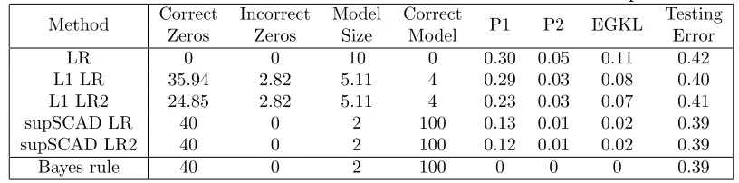
A total of 100 simulations are conducted for each procedure under all settings. Each fitted classifiers is then evaluated in terms of probability estimation and classification accuracy, as well as variable selection performance. For each method, its average testing error, P1, P2, EGKL, the number of correct and incorrect zeros, the model size, and the number of times that the true model is correctly identified are summarized in tables.

Five different procedures are considered. They are logistic regression (LR),L1 logistic

regression (L1 LR), supSCAD logistic regression (supSCAD LR), L1 LR followed by the LR (L1 LR2) and supSCAD LR followed by the LR (supSCAD LR2). In addition, we include the Bayes rule as a reference in comparison.

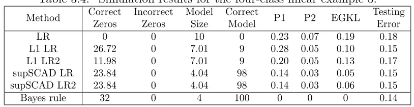
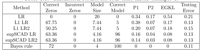
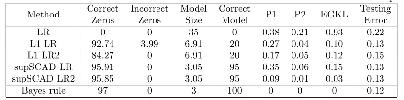
3.5.1 Four-Class Linear Example 1

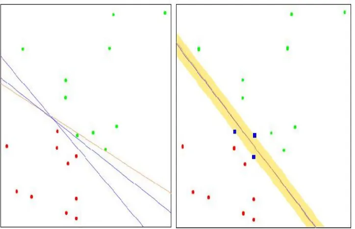
Consider a four-class example with 20-dimensional input vector x. For each class k = 1,2,3,4, the first two components of x are generated from N(µk,2I2), where µ1 =

(√2,√2)T, µ2 = (−

√

2,√2)T, µ3 = (−

√

2,−√2)T, µ4 = (

√

2,−√2)T and I2 is a 2×2 identity matrix. The remaining eighteen components are i.i.d. generated from N(0,1). Here the sample size is n = 200 for training data, and n0 = 40,000 for testing data. Evidently, only the first 2 components of xare relevant to classification, whereas the re-maining 18 components are redundant. Figure 3.1 is a plot of a randomly chosen training set. The solid lines are the Bayes boundaries.

Table 3.1 presents the results for five logistic regression variants. Entries in the last four columns have standard errors in the range of 0.001 to 0.01. The performance from Bayse method is listed on the last line as a reference to the best we can expect.

Sparse Learning in Multiclass Problems.

ABSTRACT

DEDICATION

ACKNOWLEDGEMENTS

TABLE OF CONTENTS

LIST OF TABLES

LIST OF FIGURES

Chapter 1

Review for Classification Problems

1.1

The Bayes Classifier

1.2

Linear Discriminant Analysis (LDA) and Quadratic

Discriminant Analysis (QDA)

1.3

Logistic Regression

1.4

Support Vector Machine

1.4.1

Binary SVM

1.4.2

Multicategory SVM

1.4.3

Multicategory PSVM

Chapter 2

Review for Variable Selection in

Classification Problems

2.1

L

Logistic Regression

2.2

L

SVM and

L

MSVM

2.3

SCAD SVM

2.4

Supnorm MSVM

Chapter 3

New Variable Selection Method for

Multi-class Probability Estimation

3.1

supSCAD Logistic Regression

3.2

Computation Algorithm

3.2.1

Quadratic Approximation for Log-likelihood

3.2.2

Optimization Schemes for supSCAD Logistic Regression

3.3

Extensions to Nonlinear Classification

3.4

Asymptotic Properties

3.5

Simulation Studies

3.5.1

Four-Class Linear Example 1