Some simple methods for estimating intraindividual variability in nonlinear random effects models

Some Simple Methods for Estimating Intraindividual Variability

in Nonlinear Random Effects Models

Marie Davidian

Department of Statistics, North Carolina State University Raleigh, North Carolina 27695-8203

and

David M. Giltinan

Medical Research Division, American Cyanamid Company Pearl River, New York 10965

SUMMARY

Three methods are proposed to improve both population and individual inference within the nonlinear random coefficient regression framework by incorporating possible heterogeneity in the intraindividual variance structure. These methods extend existing variance function estimation techniques by pooling information across individuals. The methods are appropriate when it is reasonable to assume

that there exists a common intraindividual variance structure. Two common situations in which this assumption may be reasonable are in pharmacokinetic modeling and in the analysis of assay data. The proposed methods are illustrated using examples from both of these fields.

Key words: Generalized least squares; EM algorithm; Heteroscedasticity; Interexperiment

A common situation in the biological and physical sciences is that in which repeated measurements are taken on each member of a sample of n individuals from a population of

interest. "Individuals" may be humans, animals, batches of material, laboratories, or experiments, and repeated measurements may be taken over time or some other set of conditions such as doses. A popular approach in the recent literature has been to represent

data of this kind by random coefficient regression models which accommodate both variation among measurements within an individual as well as individual-to-individual variation. A common phenomenon is a systematic relationship between the intraindividual variation and the level of the response. In this article, we describe simple approaches to estimation in these models which take account of this feature. We motivate our discussion by considering two examples from the specific fields of pharmacokinetic modeling and assay development, but the

methods propos~dare broadly applicable.

Table 1 presents data taken from a study of the pharmacokinetics of indomethacin following a bolus intravenous injection in 6 human volunteers (Kwan et al., 1976). For each

subject, plasma concentrations (Jig/ml) of indomethacin were measured repeatedly at 11 time points ranging from 15 minutes to 8 hours post-injection. Figure 1 shows profiles plotted by subject, suggesting that the pharmacokinetic behavior for each subject may be reasonably described by a biexponential model but that the parameters of the model may vary from subject to subject. Data from such a study may be used to address two broad objectives: the investigation of population pharmacokinetic behavior and the characterization of individual pharmacokinetic response with a view to determining suitable individual dosage regimens.

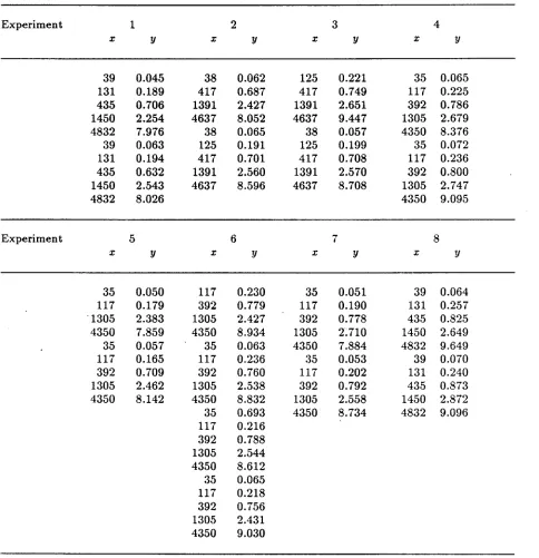
The data in Table 2 were obtained during development of an HPLC assay for an experimental drug extracted from plasma. For each of 8 experiments, a reference curve was

generated by obtaining replicate measurements (integrated area counts) at each of several known concentrations (Jig/ml) of the drug. The resulting profiles are displayed in Figure 2 and indicate that a straight line may provide an adequate characterization of the dose-response

relationship for a given experiment where the specific nature of the line exhibits variation from experiment to experiment. In assay development, prediction and calibration are primary objectives, requiring a clear understanding of both variability across experiments and the nature of within-experiment variability.

Systematic relationship between mean 'and variance of data within su bjects is a commonly recognized phenomenon in pharmacokinetic studies (Kramer et aI., 1974; Peck et aI., 1984; Beal and Sheiner 1988). Similarly, assay data collected within a single experiment are widely acknowledged to exhibit such a pattern of heterogeneous variation (Rodbard and Frazier, 1975; Finney 1976; Raab, 1981). For the indomethacin data, standardized residuals from individual ordinary nonlinear least squares fits to each profile plotted against predicted values in Figure 3 indicate the existence of an increasing relationship between variability and mean plasma level within each subject.

A

similar plot for the HPLC assay data (Figure 4) reveals a comparable pattern.

Interindividual variability is accommodated in the random coefficients framework by allowing different regression parameters for each individual. From the preceding examples, it is clear that a satisfactory model should also allow for the possibility of heterogeneous intraindividual variability ,see, for example, Beal and Sheiner (1982). In Section 2, we specify such a class of parametric models. A more precise characterization of intraindividual variability should lead to better inference on individuals and thus also improve the quality of inference regarding population parameters. In Section 3, we discuss recently proposed approaches to estimation and inference within this class. A variety of techniques exists for estimating the relationship between intraindividual variation and mean response based on data for a single individual. Section 3 also provides a brief overview of these methods. In Section 4, we describe a simple extension of these ideas to incorporate information about intraindividual variability across individuals. The methods are appropriate in cases where it is reasonable to

techniques are illustrated using the indomethacin and HPLC assay data in Section 5, and their performance is evaluated via Monte Carlo methods in Section 6. Computational details are discussed in the Appendix.

2.

A Heteroscedastic Random Coefficient Regression Model

Let Yij denote the jth response (j

=

1, ... , mi) for the ith individual (i

=

1, ... ,n). We assume that the relationship between Yij and a vector of covariates Xij may be represented according to the equation

(2.1)

In this model, f is a possibly nonlinear regression function depending on _{l3 i} (p x 1), the vector of regression parame"ters specific to the ith individual. To account for variation in the population of individuals, the l3_i are assumed to be random variables from a distribution with mean

13

and covariance matrix E; the usual specification is that of a p-variate normal distribution. The tij correspond to the intraindividual errors, and are assumed to be independent and identically distributed with zero mean and variance 1, and furthermore independent of the {3j. The additional assumption of normality of the (jj is often reasonable in

applications, particularly in the analysis of pharmacokinetic and assay data. Possible heterogeneity of intraindividual variance is accounted for by the scale parameter rr and a varIance function g depending on the conditional mean _{f(Xij,l3 i )} and a parameter () (q x 1), that is,

(2.2)

In pharmacokinetics and assay applications, the variance model is often thought to be a function of the mean JJij

=

f(xij'

f3

_{i ); a common choice is the power model}

(2.3)

see, for instance, Beal and Sheiner (1988) or Rodbard and Frazier (1975). Other models which have been proposed include the exponential model g(JJij'O)

=

exp(0 JJij)' the components of variance model g(JJij'O) = 0₁

+

JJ~l,

or the quadratic model g(JJij' 0) = 01

+

O2JJij

+

JJ;j; see Carroll and Ruppert (1988, chap. 3) for a general discussion. This framework

allows considerable flexibility in characterizing the intraindividual variability through specification of the function g and the variance parameter O. The dimension of 0 is usually chosen to be low, providing a parsimonious description of the heterogeneity of variance. The functional form of g is assumed to be known, but in many applications, the analyst may n~t be able to~specify an appropriate value for O. For a new assay, full character of variability may not be well understood; for certain assays the power model is used with 0 c: [0.6,0.9] (Finney,

1976), so that common choices 0

=

0.5 or 1.0 may be inappropriate. Beal and Sheiner (1988) caution that the pharmacokineticist's common choice 0

=

1.0 in the power model may not always be realistic. In a quadratic or exponential model, it may be difficult to specify a value for 0 a priori. In such cases a reasonable strategy is to estimate 0 from the data. Estimation of (J based on data from a given individual has received considerable attention in the literature, see Davidian and Carroll (1987) for a review. Methods for estimation of (J in the context of model (2.1) have not been examined as fully.

appropriate in all contexts. Lindstrom and Bates (1990) consider a model similar to (2.1), but with a more flexible parameterization of fj however, they do not discuss possible dependence of heterogeneity of intraindividual variability on the conditional mean. Racine-Poon (1985) and Steimer et al. (1984) assume the structure (2.1), but again, heterogeneity of intraindividual variability is not explicitly addressed. Beal and Sheiner (1982) do allow for the type of conditional variance structure (2.2), including the possibility of unknown (), and propose a normal likelihood-based approach to estimation based on a linearization of (2.1). Their method has been implemented in the computer package NONMEM (Beal and Sheiner, 1980).

Within the framework of (2.1), two types of inference may be of interest. Precise estimation of the population parameters

13

and E allows inference regarding population characteristics. For example, in pharmacokinetic studies, interest may focus on the average kinetic behavior of the drug in the target population as well as on the intersubject variation about the average,- In this case, the individual parameter values

13;

are of interest only in as much as they provide information on the population values

13

and E. In other settings, inference about individual regression parameters

13;

may be the primary focus. For instance, the pharmacokinetic parameters of an individual subject may be of intrinsic interest to help determine an individualized dosage regimen based on that subject's pharmacokinetic profile. In assay development, prediction and calibration for a given experiment will typically involve reference to the standard curve obtained for that particular experiment, so precise

characterization of

13;

is essential. A clear understanding of the nature of intraindividual variation is necessary to ensure good inference about individual parameters, particularly for prediction and calibration. Inference on population parameters often employs individual parameter estimates as building blocks, which further strengthens the case for obtaining the best possible estimates of the

13;.

is important to support high-quality inference about the regression relationship and may be of interest in its own right in the context of prediction and calibration. We propose a class of methods which provides a simple alternative to the joint maximum likelihood approach of Heal

and Sheiner (1982). In particular, our techniques are easily computed and may alleviate the computational burden sometimes encountered in the NONMEM system (Steimer et al. 1984; Racine, Grieve, and Fluhler 1986).

3.

Existing Estimation Methods

Data arising in the repeated measurement context may be classified into two broad categories: (i) those for which relatively few measurements are available on each of many individuals, and (ii) those for which many measurements are taken from each of a small number of subjects. In the first case, it may be difficult and in some i,nstances impossible to obtain good individual estimates of the

l3

i • For" data of this type, interest is usually restricted

to population parameters. For instance, Zeger, Lia~g, and Albert (1988) discuss population inference for this type of longitudinal data, such as those arising in epidemiological studies.

Similarly, Heal and Sheiner (1982) focus on estimation of population kinetics from routine clinical data, where data on individual patients are typically sparse. Data of the second type afford the opportunity to characterize the regression relationship within individuals by allowing estimation of the individ ual

13

i' The methods we propose for estimation in (2.1) are

appropriate for data of the second type for which such individual estimates are available.

3.1 Estimation in Nonlinear Random Effects Models

Consider the situation where sufficient data are available from the ith individual to

provide an estimate

13;

of

l3

i • Several estimation schemes have been proposed for this situation

Two-Stage Method (STS) by Steimer et al. (1984), forms estimates

t

=

n-1"t

(f3i-lJ)(f3i-lJ)T.

i=l

In this method, no refinement of the individual

f3i

such as shrinkage toward the mean is implemented, nor are possible differences in the precision of the

f3i

accounted for. Furthermore, the STS estimator for E is upwardly biased, being based on estimated quantities

f3i.

The computational simplicity of this method is, however, appealing. More complicated

methods which incorporate these features have also been proposed, and are based on the assumption that the relationship

(3.1)

holds, at least approximately. Iff is linear and

f3i

is the ordinary least squares estimator, (3.1) will hold exactly in the case of n~rmal fiji in the nonlinear case, (3.1) will be true asymptotically. Under (3.1) and normality of the

f3

i , Steimer et al. (1984) derive an iterative estimation scheme known as the Global Two-Stage method (GTS) using maximum likelihood estimation based on

f3i ,....

N(

f3

i ,Vi + E). In particular, their algorithm is an EM-type algorithm composed of the following two steps: At iteration (k+1)

1. Produce refined estimates of the

f3

i :

(3.2)

• -1 n . • • • T

E(k+1)

=

n

?:

{(.8i)(.I:+1) - .8(k+1)}{(.8i)(k+1) - .8(k+1)}

.=1

+ n-1

f:

(V;-1+E(k\)-1 .

• =1

A similar method derived from a hierarchical Bayesian perspective has been developed by Racine-Poon (1985). Note that in the linear case the GTS algorithm updates the

Pi

to the

current Bayes estimate at each iteration.

Steimer et al. (1984) and Racine-Poon (1985) mention ordinary least squares or iteratively reweigh ted least squares as possibilities for the estimates .8";. These correspond to implicit assumptions of homogeneous intraindividual variation or heteroscedasticity with () known, respectively. When () is unknown, the methods proposed in Section 4 allow () to be estimated, thereby leading to more efficient estimates .8"; which may be used as input to any of the above estimation schemes.

3.2 Estimation from Individual Data

For the case where estimation of () is to be accomplished based on data from individual i only, several methods have been proposed, see Carroll and Ruppert (1988, chap. 3). A popular method in the recent pharmacokinetics literature is simultaneous estimation of (.8j ,u, ()) by

normal theory maximum likelihood, sometimes referred to as "extended least squares (ELS)," see Peck et al. (1984). Alternatively, a very general class of methods for estimation of

(.8j 'u, ()) is that of generalized least squares (G LS). These methods can be characterized by

the following scheme:

1. Obtain an estimate of.8_i by a preliminary unweighted fit.

2. Use residuals from the preliminary fit to estimate () and u and form estimated weights based on the estimates of.8i and ().

Step 2 is nonspecific and can be implemented in practice in several ways. In this paper, we focus on three methods, all based on transformations of absolute residuals from a preliminary fit, and all relatively easy to compute using methods discussed in the Appendix.

Given a preliminary estimate of f3f, the method of pseudolikelihood (PL) minimizes in (1'

and ()

( p )

~({Yij-f(xij,f3f)}2

[ 2 2{ ( p) }])

PL i f3i ,(1', ()

=!::

2 2{r( .. at:) ()}

+

log (1' g f Xij'f3i ,() .

1-1 (1' g l'_{X S1 'l-'s ,}

(3.3)

Minimizing the objective function (3.3) corresponds to maximizing the normal theory loglikelihood evaluated at

f3f.

A fuller discussion of the motivation and properties of this method is given by Davidian and Carroll (1987).

One criticism of estimation based on (3.3) IS that it takes no account of the loss of degrees of freedom due to preliminary estimation of f3i . An alternative is to replace (3.3) by a

suitably. modified objective function. An appropriate modification may be derived using the ideas underlying restricted maximum likelihood, see Carroll and Ruppert (1988, p. 73-76) for details. We shall refer to this method as restricted maximum likelihood (REML) with

corresponding objective function

+

log det{ (Xf)T (Gf)-1 Xf},

where Xr is the (mi x p) matrix of derivatives of f(Xij,f3i) with respect to f3 i evaluated at

f3f,

possibility of a heavier-tailed distribution of the (ii' an attractive proposal is to replace the role of squared residuals by absolute residuals. Analogous to (3.3), the absolute residuals (AR)

method minimizes in 11 and 0

(fJ P

)

~(IYii-f(Xii,fJf)1

I [ {tie

fJP)

all)

ARi _i,l1,O =

l:::

_{{f( ..} fJ~) _O}

+

_{og l1g xii' i'u ,}

)_1 TJg XI)' I ,

(3.5)

where the role of U' is replaced by 11 = U'E

1

(ii

I.

Note that (3.5) can also be motivated by

considering a suitable double exponential distribution.

vYhichever of the three methods one chooses to implement in step 2 of the GLS scheme, it

IS essential to iterate the scheme so that the residuals used in estimating 0 and the weights

used in step 3 are obtained from a weighted fit. No consensus exists on a recommended number of iterations, but the need for such iteration is widely recognized, see Carroll, vYu, and Ruppert (1988).

4.

Pooled Estimation of Intraindividual Variability

In this section, a simple extension of the methods outlined ill Section 3.2 is described.

The quality of the estimates (17,0) based on data from a single individual only is unlikely to be very good. However, if data from several individuals are available, it is intuitively clear that improved estimates of intraindividual variance parameters may be obtained by pooling

information across individuals. One way of doing this is to modify the GLS procedure of Section 3.2 in a straightforward manner as follows:

1. Obtain, in n separate regressions, preliminary unweighted estimates

fJr

for each individual.

2. Estimate the variance parameters 17 and 0 by iT and

0

chosen to minimize

f:

0i(fJL

17,0),

i=l

3. Form estimated weights g-2{f(xii' ,8f),8} and re-estimate the ,8 i by n weighted regressions. Treating the results as new preliminary estimates ,8f, return to step 2.

Just as in the case of estimation for individual data only, it is essential to iterate this scheme. Our experience with pharmacokinetic and assay data indicates that convergence tends to occur

between 5 and 10 iterations.

In step 2, the objective functions in the pooled estimation scheme are identical in form to those based on individual data only. Computation of the pooled variance estimates is thus no more difficult and may be implemented by the algorithms described in the Appendix. Although we have focused on three particular choices of objective function for this step, the

algorithm is flexible in that any variance function estimation scheme based on residuals from a preliminary fit may be incorporated.

It is intuitively clear that use of information across individuals should improve characterization of the intraindividual variability_. In the examples and simulation results that follow, "we will show that this improved estimation of () translates to an improvement in the

quality of the estimates of the ,8i relative to unweighted estimates and to GLS estimates calculated separately for each individual based only on data from that individual. Use of these improved estimates as input to one of the procedures described in Section 3.1 yields an

improvement in the overall population estimates

i3

and

E.

Clearly, to obtain sensible estimates of the population parameters, E in particular, the number of individuals should not be too small.

5.

Examples

5.1 Pharmacokinetics of Indomethacin

f(t,,8)

=

/lexp(_eP2t)

+

/3

exp(-eP4t). (5.1)

This parameterization ensures that the quantities ePA:, k

=

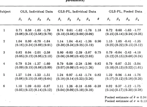
1, ... , 4, are positive and is employed so that the assumption of normality of ,8 is more likely to be fulfilled (Racine-Poon 1985). To accommodate the heteroscedasticity evident Figure 3, the power model (2.3) was assumed.

The following estimation methods were applied to illustrate the techniques. Estimation based on individual data was carried out using ordinary least squares (OLS), extended least squares (ELS), generalized least squares (GLS) using each of the three variance function estimation methods PL, REML, and AR. In addition, GLS estimates based on pooled variance estimation of 0 using PL, REML, and AR were obtained. For estimation based on individual data, results 'obtained using all four weighted methods were entirely comparable. Similarly, 'all three GLS methods based on pooled variance estimation gave virtually identical results.' Accordingly, we limit our presentation of results for these methods to those obtained using pseudolikelihood. Table 3 summarizes results obtained by OLS, by GLS-PL based on individual data, and GLS-PL based on pooled estimation ofO.

Estimates of 0 based on individual data varied considerably from subject to subject. It

seems likely that this is more a reflection of the probable unreliability of variance parameter

estimates from sparse data than of real variation in the true intrasubject error structure. Assuming that the same assay was used to obtain measurements for each subject, the supposition of a common 0 value is reasonable. The common 0 estimate obtained from pooled

GLS method was 0.94, indicating that a constant coefficient model is plausible for these data. In estimating 0, convergence of the GLS iterative scheme occurred in 3 to 6 iterations in all

cases.

estimating

p.

OLS estimates differed somewhat, with the greatest discrepancies observed in

the parameters for the second compartment,

P

3 and

P

4 • Standard errors for the OLS method should not be considered reliable, since they are predicated on an inaccurate assumption about the underlying error structure. A plot of the standardized residuals from GLS using the pooled PL estimate of 0 (Figure 5) indicates that weighting provides a more satisfactory fit to

these data.

5.2 HPLC Assay

For the assay data represented in Figure 2, a simple linear regression model for the mean response and the power model (2.3) for variance were assumed. The same estimation methods were employed as in Section 5.1. Since the three GLS methods, PL, REML, and AR again gave virtually identical results, both in the indivdual and pooled estimation cases, Table 4 includes only the results for OLS, GLS-PL, and ELS.

Inaividual estimates of 0 based on data from each experiment were fairly consistent,

although those for experiments 1 and 5 differed somewhat. This could be attributed to disparate experimental conditions; a more likely explanation IS that these estimates are not

very good, since they are based on at most 10 observations. Pooled PL estimation of

e

and the individual GLS estimates of the

Pi

converged in 6 iterations of the GLS process. The pooled estimate of 0 was again close to an apparent average across experiments, and seems to

suggest that a constant coefficient of variation model may be appropriate for this assay.

The individual estimates of the

Pi

based on OLS, ELS, and GLS based on pooled and individual estimation of 0 were all comparable in this example. The standard errors reported for OLS are again inappropriate. The beneficial effect of weighting is exhibited in the comparision between Figures 4 and 6.

as is commonly the case for HPLC assay data. However, in this particular setting, prediction and calibration are often a primary focus. For these applications, a proper characterization of the error structure is crucial. This is well illustrated in Table 5, which displays prediction intervals for experiment 1 at several concentration levels, following the different estimation schemes given in Table 4. The intervals based on OLS are of almost constant width and thus highly inappropriate. The nature of the intervals varies somewhat among the weighted schemes, particularly at the low and high concentrations, illustrating the sensitivity of prediction to characterization of variability.

6.

Simulation Results

To assess the performance of the methods proposed in this paper, we carried out a number of modest simulations. Our investigation thus far has been limited to compartmental models of the type typically encountered in pharmacokinetic analysis. The performance of the methods both in estimating population and individual parameters was examined. The simulations attempted to mimic the types of data for which population and individual

estimation would be appropriate. For instance, for population analysis to be sensible, data should be available from a reasonably large number of subjects. In all simulations, it was assumed that sufficient data were available on all subjects to allow estimation of individual pharmacokinetic parameters. Our simulation work encompassed both monoexponential and biexponential models, assuming a number of different designs and possible intraindividual error structures. For brevity, our presentation is limited to two specific biexponential cases.

Conclusions for monoexponential cases were qualitatively similar. All compuations were programmed in GAUSS and executed on IBM PCs.

6.1 Population Estimation

population parameter values:

/3

=

In [2.0, 1.5, 0.3, 1.5]T, (6.1)

0.030 0.010 -0.013 0.003 0.020 -0.016 0.000

E=

(6.2)

0.050 0.010 0.050

Each of the simulation data sets was formed as follows. Data were generated for 20 individuals with 10 observations for each individual taken at time points t = 0.25, 0.50, 0.75, 1, 1.5, 2, 3, 4, 6, and 8 hours. For each data set, individual

/3

i were generated according to a N(

/3,

I;)

distribution. For individual i, a profile was generated by adding independent normal intrasubject errors generated according to a power model (2.3) with rr

=

0.05 and 0

=

1.0 to the regression model f(t_ii

,/3i)'

Fifty such data sets, each consisting of 20 individual profiles, were simulated.

Individual estimates were obtained for each data set by each of the following methods: (1) ordinary (unweighted) least squares (OLS)

(2) generalized least squares assuming () specified to be the true value 1.0 (GLS-T) (3) generalized least squares assuming () wrongly specified to be equal to 0.5 (GLS-M)

(4) generalized least squares, () estimated by pseudolikelihood based on individual data (GLS-PL)

(5) generalized least squares, () estimated by absolute residuals based on individual data (GLS-AR)

(6) generalized least squares, () estimated by restricted maximum likelihood based on individual data (GLS-REML)

(8) generalized least squares, (J estimated by pseudolikelihood based on pooled estimation (GLS-PLPOOL)

(9) generalized least squares, (J estimated by absolute residuals based on pooled estimation (GLS-ARPOOL)

(10) generalized least squares, (J estimated by restricted maximum likelhood based on pooled estimation (GLS-REMLPOOL).

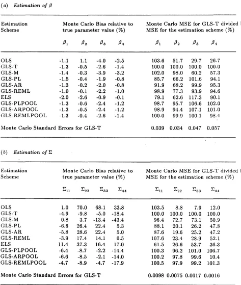
Population estimates of (3 and r; were obtained for each of these methods by using both the STS and GTS schemes. Conclusions regarding the relative merits of methods (1) - (10) for estimation of (3 were similar for both STS and GTS. For STS, a severe upward bias was apparent in the estimation of r; for all methods, as expected. Accordingly, we present comparisons of(1) - (10) for population estimation only for GTS.

Tables 6 (a) and (b) exhibit the salient features of simulation results. It is evident from Table 6 (a) that there is little distinction among the methods with respect to bias in the estimation of (3. Since weighting according to the correct value of (J is theoretically optimal, GLS-T may be regarded as a benchmark in gauging the efficiency of the other methods. Accordingly, the Monte Carlo mean square error (MSE) for each method has been expressed relative to that for GLS-T in Table 6 (a). Clearly, using individual estimates obtained by OLS as input to the GTS algorithm can result in highly inefficient estimation of (3. Misspecification of (J can also lead to inefficient estimation of (3. ELS and GLS methods based on individual data result in improved efficiency but do not match the performance of the GLS methods which pool information across individuals. It is evident from the table that, under the conditions in this simulation, the efficiency attained by the pooled GLS procedures almost reaches the theoretically optimal performance of GLS-T.

not surprising in view of the limited sample size. Substantial biaS in estimating the variances was observed for all methods, with that for OLS being particularly severe. Of the remaining methods, none appeared clearly superior, though the pattern for the three pooled GLS methods appeared to match that of GLS-T most closely. We note that in limited simulations involving monoexponential regression models, the degree of bias observed in estimation of the three elements of E was much less severe. Inspection of the MSE values expressed relative to those for GLS-T again reveals the poor performance of OLS. Methods based on individual data only also showed poor performance. The performance of pooled GLS methods, in contrast, matched that of GLS-T.

A general message from Tables 6 (a) and (b) is that the paucity of information .on intrasubject variability for any individual subject may exact a price. Specifically, all four

methods which rely on individual subject data to characterize the weighting scheme involve some loss of efficiency, especially in estimation of E. For the design considered in this simulation (20 subjects, 10 observations per subject), pooling information on intraindividual variability to obtain the correct weighting scheme offers a substantial gain in efficiency.

'vVe also simulated 50 data sets according to the same model, parameter values, and error structure, but modified the design to one with 20 subjects and 19 observations per subject. In this case, the advantage of the pooled GLS methods over those based on individual subject data was much less pronounced. This is not surprising, since, if 19 observations per subject really were available, one could expect a good characterization of the error structure based on data from a single subject. However, we feel that this situation is unlikely to occur in practice. Accordingly, the advantage offered by the pooled estimation methods is likely to be of practical import.

For purposes of estimating

f3

and E, the choice of method for pooled estimation of0 was .

of little consequence. In situations where estimation of 0 is of primary concern, as in the

context of prediction and calibration, it is of interest to distinguish among the three methods.

Pooled estimation of () based on restricted maximum likelihood (REMLPOOL) proved superior to that based on pseudolikelihood or absolute residuals, both in terms of bias and MSE. The latter methods exhibited Monte Carlo biases on the order of 8% to 10% of the true value, while that for REMLPOOL was less than 1%. In addition, REMLPOOL displayed a clear advantage with respect to MSE, offering a reduction by a factor of 3 to 4 over the other two

methods.

6.2 Individual Estimation

To assess the effect of different estimation methods on the quality of inference about individual subjects, the following simulation was performed. First, ten individual parameters J3_i were generated from a N(J3,E) distribution with

J3

and E as in (6.1) and (6.2). These parameter values were regarded as coming from fixed subjects about whose parameters inference was to be made. Fifty data sets were simulated, each consisting of a profile for each of the "ten subjects generated according to the normal intraindividual error structure (power model with () = 1, (J' = 0.05) and ten point sampling schedule described in Section 6.1. Each of

methods (1) - (10) was used to obtain individual estimates of the

J3

i - Refined estimates of the J3i were also obtained for each method by application of the GTS algorithm as specified by

(3.2). Our interest in this simulation focused only on the quality of inference regarding the ,8i

attained by each of the ten methods, both unaltered and incorporating the Bayesian

adjustment towards the mean.

With ten subjects and ten observations per subject, MSEs for the Bayesian versions of each of the ten procedures were lower than their unadjusted counterparts for each subject. This reflects the standard Bayesian view that if information on anyone individual is sparse, under the assumptions of the model, one may gain in efficiency by borrowing information from the remaining subjects. In a simulation with more observations (19) available per subject and

was almost entirely eliminated for all methods.

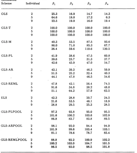
Comparison among the methods (1) - (10) gave similar results for both unadjusted and refined versions. For brevity, we present comparisons only for the refined estimators (Table 7). Rather than show results for all ten, Table 7 gives MSE comparisons for three randomly chosen subjects which are representative of results for the full data set. As before, MSEs are expressed relative to those for generalized least squares assuming () correctly specified (G LS-T). In general, the performance of OLS was very poor for all subjects. For generalized least squares with () misspecified (GLS-M), efficiency was occasionally quite low. Methods involving weighting based on individual data only (GLS-PL, GLS-AR, GLS-REML, ELS) performed uniformly poorly. In contrast, when weighting was accomplished incorporating information pooled across subjects, efficiency was typically close to that of GLS-T. This simulation and others not reported here bear out the intuitive idea that better inference may be achieved by using the information on intraindividual variability provided by all subjects.

7.

Discussion

We have proposed methods to improve both population and individual inference within the nonlinear random coefficient regression framework. These methods extend existing

variance function estimation techniques in an entirely straightforward manner. A key assumption for the methods to be useful is that there exist a common intraindividual variance structure, since otherwise the pooling of information across individuals, which is the foundation of the methods, is not necessarily appropriate. Two common situations in which this assumption may be reasonable are in pharmacokinetic modeling and in the analysis of assay data. The validity of this assumption should be critically examined by the data analyst in any given situation.

These are open to criticism on two grounds, particularly in the context of pharmacokinetic modeling. First, given the sparsity of data typically available for an individual subject and the need to estimate anywhere from two to six regression parameters, it may be too much to ask

that reliable information on weighting be obtained from a single subject's profile. Second, use of these methods in a typical pharmacokinetic analysis such as the indomethacin data results in a different weighting scheme for each individual (reflecting the different individual estimates of 8). This may not be desirable from a practical point of view. The pooled estimation methods described in Section 4 alleviate this problem and are no more difficult to compute. vVe remark that, although a constant coefficient of variation model for intraindividual variance

seemed reasonable in the examples discussed here, this need not always be the case. Estimation of intraindividual variance parameters is useful both in assessment of the

appropriateness of standard models for variance and in determining when other models may be more reasonable than those usually adopted.

vVe have not included the first order linearization method of Heal and Sheiner (1982) that

IS implemented in the NONMEM package (Heal and Sheiner 1980). The methods discussed

above are generally simpler in implementation and philosophy, and inclusion of the NONMEM scheme lies beyond the scope of the current investigation.

No simulation can provide a complete investigation of the properties of any estimation scheme. However, our experience, mainly with the polyexponential regression models and the power variance function frequently employed in pharmacokinetic analysis, suggests that the

ACKNOWLEDGEMENT

The authors are grateful to Dr. J. Hubbell, Department of Medicinal Biochemistry, Burroughs Wellcome Co., Research Triangle Park, North Carolina, for providing the HPLC assay data.

REFERENCES

Beal, S.L. and Sheiner, L.B. (1980). The NONMEM system. The American Statistican 34,

118.

Beal, S.L. and Sheiner, L.B. (1982). Estimating population kinetics. CRC Critical Reviews in Biomedical Engineering 8, 195-222.

Beal, S.L. and Sheiner, L.B. (1988). Heteroscedastic nonlinear regression. Technometrics 30,

327-338.

Carroll, R.J. and Ruppert, D. (1988). Transformation and Weighting in Regression. New York: Chapman and Hall.

Carroll, R.J., Wu, C.F.J., and Ruppert, D. (1988). The effect of estimating weights m weighted least squares. Journal of the American Statistical Association 83. 1045-1054.

Davidian, M. and Carroll, R.J. (1987). Variance function estimation. Journal of the American Statistical Association 82, 1079-1091.

Finney, D.J. (1976). Radioligand assay. Biometrics 32, 721-740.

Giltinan, D.M. and Ruppert, D. (1989). Fitting heteroscedastic regression models to individual pharmacokinetic data using standard statistical software. Journal of Pharmacokinetics and Biopharmaceutics 17, 601-614.

Kramer, W.G., Lewis, R.P., Cobb, T.C., Forester, W.F., Visconti, J.A., \-Vanke, L.A., Boxenbaum, H.G., and Reuning, R.H. (1974). Pharmacokinetics of digoxin: comparison of a two- and three-compartment model in man. Journal of Pharmacokinetics and Biopharmaceutics 2, 299-312.

Kwan, K.C., Breault, G.O., Umbenhauer, E.R., McMahon, F.G., and Duggan, D.E. (1976). Kinetics of indomethacin absorption, elimination, and enterohepatic circulation in man.

Journal of Pharmacokinetics and Biopharmaceutics 4, 255-280.

Lindstrom, M.J. and Bates, D.M. (1990). Nonlinear mixed effects models for repeated measures data. Biometrics 46, in press.

Peck, C.C., Beal, S.L., Sheiner, L.B. and Nichols, A.I. (1984). Extended least squares nonlinear regression: a possible solution to the choice of weights problem in analysis of individual pharmacokinetic data. Journal of Pharmacokinetics and Biopharmaceutics 12,

Raab, G.M. (1981). Estimation of a variance function, with ap})lication to radioimmunoassay. Applied Statistics 30, 32-40.

Racine, A., Grieve, A.P. and Fluhler, H. (1986). Bayesian methods in practice: experiences in the pharmacuetical industry. Applied Statistics 35, 93-150.

Racine-Poon, A. (1985). A Bayesian approach to nonlinear random effects models.

Biometrics 41, 1015-1023.

Rodbard, D. and Frazier, G.R. (1975). Statistical analysis of radioligand assay data.

Methods of Enzymology 37,3-22.

Steimer, J.L., Mallet, A., Golmard, J.L. and Boisvieux, J.F. (1984). Alternative approaches to estimation of population pharmacokinetic parameters: comparison with the nonlinear mixed effect model. Drug Metabolism Reviews 15, 265-292.

Zeger, S.L., Liang, K. and Albert, P. (1988). Models for longitudinal data: a generalized estimating equation approach. Biometrics 44, 1049-1060.

APPENDIX

Computational Aspects

Minimization of the pseudolikelihood objective function (3.3) based on data from individual i may be accomplished by minimizing the sum of squares

where [Jij

=

f(xij,Pf), gij(B)

=

_{g{f(xij,Pf),B}, and gi(B) is the geometric mean of the m i} gij(B) values. This may be implemented by regressing a dummy variable u which is identically zero on the "regression function"

gi(B)(yij - [Jij) gi/ B)

(Carroll and Ruppert, 1988, p. 72). Similarly, the objective function (3.4) for restricted maximum likelihood is minimized by regressing u on

{g;i(B)}mi/(m;-p\Yij - [Jij)[det{(

xf)

T(Gn-1

xf}

]1/2(mi -p)

To minimize the absolute residuals objective function (3.5), regress u on

Extension of this principle to the pooled estimation case is immediate. Define g( (}) to be the geometric mean of the N gij((}) values, N

=

E?mi' Then the pooled estimate of (} based on pseudolikelihood may be shown to minimize

(A.l)

To achieve this, regress a dummy variable identically equal to zero on the function in braces in (A.l). Extension of the restricted maximum likelihood and absolute residual methods to the

pooled "estimation case is accomplished in a similar fashion.

In two common special cases, the power and exponential variance functions, the relevant dummy variable regressions for the pseudolikelihood and absolute residual methods can be carried out using any standard nonlinear least squares package. Giltinan and Ruppert (1989) give details of implementation using PROe NLIN in the SAS Software System (SAS

Institute). The limitation to these special cases and the inability to implement the restricted

INDOMETHACIN

0

1'0

r-...l() _{Eech symbol represents e different subject}

E N

'-...

CJ"l0

::i..

'-.-/N

Z

Ol()

f-"':

«

n:::

f-ZC::

w~ U Z

Ol()

00

0 .~.~-. .-.

0 0 _{2 3 4 5 6 7 8 9}

TIME

(hou rs)

0

CJ)

~co

0

Q)

I...r---0

....-w

CD

U1

ZtD

0

0.... v U1

W

0:::1'0

N

-o~

0

Each symbol r-epresents

It different experiment

2 3

CONC.

Cug/ml)

4 5

I

OLS RESIDUALS-INDOMETHACIN

CD,.---""T""---,~---r---...,.----___.

Each symbol represents

..r 8 differerTt subject

o

. N

•

0

0 X

+

-

_Iv

₀

₊

(j) t:.'1

W

~x

+25

•

et::O

_'10 '1 _t:.

+

'1 '1

0

•

+

t:. _X

+

₀

~

•

UlN

I

..r

I 0

CD

I 0.0

_0.5

_1.0

_1.5

2.0 '} r:;

"-.- '

PRED. VALUE

Each symbol represents a different experiment

.N

o

(f)

~o'f

o

I-C/lN

I

..r

I

t:::.

~+

x·

•

~

\l

X _\l

X

X

•

\l

0

+t:::.

!II

11 10

9 8

4- 5 · 6 7

PRED. VALUE

3

2

t . O I - _ - ' -_ _'--_...J...._----'_ _..._ - - '_ _...J.-_--l._ _...J-._---l._---'

I 0

GLS RESIDUALS-INDOMETHACIN

C D r - - - r - - - " " " " ' T - - - r - - - " " " T ' " - - - ,

BASED ON POOLED ESTIMATION OF 8

0

. N

•

0

0

•

-V

•

-~ 0

X

\l

(f)

W _{151 0}

t::,.

₊

₊

cr:o

~

.xt::,.x

\l0 "V

_t::,.X+.

t::,.

+t::.x

\l

•

₀

0

TID

~

+

\-UlN

•

I 0

~

I _{Each symbol represents}

a different subject

2.5 2.0

1.0 1.5

PRED. VALUE

0.5

CDL- -..l.- ----l. ..L- ----L ~

I 0.0

GLS RESIDUALS-HPLC ASSAY

•

•

1

_o

~

BASED ON POOLED ESTIMATION OF G

A

X.

0'1

+J+

_tT

t

· 0 A

><'i1

'V

₊

•

"*"

I _{Each symbol represents} a different experiment

11 10

9 8

4 5 6 7

PRED. VALUE

3

2

r i ) 1 - _ - l - _ - - - L_ _..l..-_...J..._ _I....-_....1.-_---l-_ _. l . . - _ - - l - _ - - ' _ - - '

I 0

Table

l.

Plasma concentrations (JJgI ml) of indomethacin following single intravenous dose (Kwan et al. 1976)

Time Subject

(min) 1 2 3 4 5 6

15 1.50 2.03 2.72* 1.85 2.05 2.31

30 0.94 1.63 1.49 1.39 1.04 1.44

45 0.78 0.71 1.16 1.02 0.81 1.03

60 0048 0.70 0.87 0.89 0.39 0.84

75 0.37 0.64 0.80 0.59 0.30 0.64

120 0.19 0.36 0.39 0040 0.23 0042

180 0.12 0.32 0.22 0.16 0.13 0.24

240 0.11 0.20 0.12 0.11 0.11 0.17

300 0.08 0.25 0.11 0.10 0.08 0.13

360 0.07 0.12 0.08 0.07 0.10 0.10

480 0.05 0.08 0.08 0.07 0.06 0.09

y

=

response (integrated area count)

Experiment 1 2 3 4

x y x y x y x Y

39 0.045 38 0.062 125 0.221 35 0.065

131 0.189 417 0.687 417 0.749 117 0.225

435 0.706 1391 2.427 1391 2.651 392 0.786

1450 2.254 4637 8.052 4637 9.447 1305 2.679

4832 7.976 38 0.065 38 0.057 4350 8.376

39 0.063 125 0.191 125 0.199 35 0.072

131 0.194 417 0.701 417 0.708 117 0.236

435 0.632 1391 2.560 1391 2.570 392 0.800

1450 2.543 4637 8.596 4637 8.708 1305 2.747

4832 8.026 4350 9.095

Experiment 5 6 7 8

x y x y x y x y

35 0.050 117 0.230 35 0.051 39 0.064

117 0.179 392 0.779 117 0.190 131 0.257

"1305 2.383 1305 2.427 392 0.778 435 0.825

4350 7.859 4350 8.934 1305 2:710 1450 2.649

e

35 0.057 35 0.063 4350 7.884 4832 9.649

117 0.165 117 0.236 35 0.053 39 0.070

392 0.709 392 0.760 117 0.202 131 0.240

1305 2.462 1305 2.538 392 0.792 435 0.873

4350 8.142 4350 8.832 1305 2.558 1450 2.872

35 0.693 4350 8.734 4832 9.096

Table 3.

Parameter estimates, Indomethacin data (standard errors given in parentheses)

Subject OLS, Individual Data GLS-PL, Individual Data GLS-PL, Pooled Data (J

1 0.71 0.58 -1.65 -1.79 0.74 0.61 -1.62 -1.76 1.18 0.72 0.60 -1.63 -1.77 (0.08) (0.12) (0.58) (0.79) (0.10) (0.08) (0.09) (0.09) (0.15) (0.14) (0.24) (0.25) 2 1.04 0.80 -0.70 -1.64 1.14 1.04 -0.41 -1.36 0.90 1.15 1.05 -0.41 -1.35

(0.16) (0.34) (0.69) (0.91) (0.38) (0.34) (0.25) (0.19) (0.25) (0.22) (0.15) (0.12) 3 0.82 0.04 -2.01 -2.58 0.80 -0.03 -2.39 -3.87 0.75 0.79 -0.04 -2.43 -4.18

(0.05) (0.12) (0.95) (2.10) (0.06) (0.08) (0.43) (2.93) (0.12) (0.15) (0.68) (6.24) 4 0.79 0.24 -1.37 -1.60 0.79 0.08 -2.28 -2.96 0.82 0.79 0.07 -2.31 -3.04

(0.09) (0.15) (0.88) (0.89) (0.07) (0.09) (0.44) (1.26) (0.10) (0.13) (0.52) (1.61) 5 1.27 1.04 -1.23 -1.51 1.24 0.97 -1.43 -1.74 0.82 1.22 0.96 -1.44 -1.76

(0.08) (0.15) (0.49) (0.64) (0.18) (0.14) (0.23) (0.26) (0.17) (0.12) (0.18) (0.20) 6 1.10 1.09 -0.03 -0.87 1.11 1.26 -0.18 -0.66 -0.38 0.92 0.37 -1.12 -1.75

parentheses)

Exper- OLS, Individual GLS-PL, Individual ELS, Individual GLS-PL, Pooled

iment Data Data Data Data

/3

1

/3

2

/3

1

/3

2 ()

/3

1

/3

2 ()

/3

1

/3

2

1 -0.026 1.662 -0.013 1.649 0.614 -0.013 1.649 0.614 -0.011 1.630 (0.030) (0.014) (0.007) (0.027) (0.006) (0.024) (0.004) (0.031) 2 -0.026 1.801 -0.005 1.756 0.874 -0.006 1.758 0.868 -0.005 1.762

(0.065) (0.028) (0.004) (0.037) (0.003) (0.032) (0.004) (0.034) 3 -0.071 1.969 -0.013 1.829 1.158 -0.013 1.829 1.164 -0.018 1.895

(0.088) (0.039) (0.003) (0.043) (0.002) (0.038) (0.005) (0.036) 4 -0.018 2.009 -0.003 2.032 0.957 -0.003 2.032 0.958 -0.003 2.033

(0.073) (0.036) (0.002) (0.030) (0.002) (0.027) (0.004) (0.038)

5 -0.016 1.845 -0.017 1.845 0.509 -0.017 1.846 0.508 -0.013 1.821 (0.035) (0.016) (0.007) (0.020) (0.006) (0.018) (0 ..004) (0.036) 6 -0.050 2.038 -0.003 1.968 1.004 -0.003 1.968 1.005 -0.004 1.981

(0.031) (0.015) (0.002) (0.020) (0.002) (0.019) (0.003) (0.027) 7 -0.025 1.912 -0.017 1.957 1.007 -0.017 1.958 1.005 -0.017 1.962

(0.090) (0.044) (0.003) (0.047) (0.003) (0.042) (0.004) (0.037) 8 -0.013 1.940 -0.008 1.942 0.934 -0.008 1.942 0.934 -0.008 1.939

Table

5.

Prediction intervals for single future measurement for selected concentrations, HPLC assay data

Estimation Scheme concentration (x) x 1000

25 100 500 1000 2000 5000

OLS, Individual Data

Lower Limit -0.189 -0.064 0.603 1.436 3.097 8.049

Upper Limit 0.220 0.344 1.006 1.836 3.498 8.516

GLS-PL, Individual Data

Lower Limit 0.004 0.100 0.671 1.417 2.938 7.577

Upper Limit 0.051 0.202 0.950 1.853 3.629 8.882

ELS, Individual Data

Lower Limit 0.007 0.106 0.686 1.440 2.975 7.647

Upper Limit 0.049 0.197 0.936 1.830 3.593 8.812

GLS-PL, Pooled Data

Lower Limit 0.019 0.123 0.686 1.405 2.859 7.276

algorithm using as input individual estimates obtained by several estimation schemes

( a) Estimation of{3

Estimation Monte Carlo Bias relative to Monte Carlo MSE for GLS-T divided by

Scheme true parameter value (%) MSE for the estimation scheme (%)

{31 {32 {33 {34 {31 {32 {33 {34

OLS -1.1 1.1 -4.0 -2.5 103.6 51.7 29.7 26.7

GLS-T -1.3 -0.5 -2.6 -1.4 100.0 100.0 100.0 100.0

•

GLS-M -1.4 -0.3 -3.9 -3.2 102.0 98.0 60.2 57.3

GLS-PL -1.5 -0.4 -1.9 -0.8 85.7 66.2 101.6 94.1

GLS-AR -1.3 -0.2 -2.0 -0.8 91.9 68.2 99.9 95.3

GLS-REML -1.0 -0.1 -2.2 -1.0 98.9 77.3 93.9 94.6

ELS -2.0 -2.6 -0.9 -0.1 79.1 62.6 117.3 90.1

GLS-PLPOOL -1.3 -0.6 -2.4 -1.2 98.7 95.7 106.6 102.0

GLS-ARPOOL -1.3 -0.5 -2.4 -1.2 98.9 94.4 107.1 101.0

GLS-REMLPOOL -1.3 -0.4 -2.6 -1.4 100.0 99.9 100.1 98.4

Monte Carlo Standard Errors for GLS-T 0.039 0.034 0.047 0.057

(b) Estimation of:E

e

Estimation Monte Carlo Bias relative to Monte Carlo MSE for GLS-T divided by

Scheme true parameter value (%) MSE for the estimation scheme (%)

:Ell E22

'"

....33 E44 Ell En E33 :E44

OLS 1.0 70.0 68.1 33.8 103.5 8.8 7.9 12.0

GLS-T -4.9 -9.8 -5.0 -18.4 100.0 100.0 100.0 100.0

GLS-M 0.8 3.7 -13.4 -43.4 96.4 72.7 73.1 50.9

GLS-PL -6.6 26.4 22.4 5.3 88.1 20.1 26.2 47.8

GLS-AR -5.8 28.6 22.4 5.0 87.6 19.6 25.2 47.2

GLS-REML -3.9 17.4 14.1 0.5 107.6 23.4 28.9 52.1

ELS 11.4 37.3 16.4 17.0 61.5 26.6 53.7 36.3

GLS-PLPOOL -6.4 -8.7 -2.2 -14.4 100.3 96.2 101.0 106.7

GLS-ARPOOL -6.6 -8.5 -2.1 -14.0 100.2 97.8 99.6 10.4

GLS-REMLPOOL -4.7 -8.9 -4.7 -17.9 100.5 97.9 99.2 101.3

Table 7.

Simulation results for refined estimation of individual regression parameters

/3

i

for 3 randomly selected individuals from 10 simulated individuals

Monte Carlo MSE for GLS-T divided by MSE for the estimation scheme expressed as %

Estimation

Scheme Individual

_/31

/3

2

/33

/34

OLS 2 25.3 16.9 14.7 14.3

5 64.6 18.0 17.2 6.3

9 22.5 19.9 16.0 19.4

GLS-T 2 100.0 100.0 100.0 100.0

5 100.0 100.0 100.0 100.0

9 100.0 100.0 100.0 100.0

GLS-M 2 40.3 53.5 87.5 93.6

5 86.0 71.0 85.3 67.7

9 36.4 59.6 110.6 130.5

GLS-PL 2 41.9 38.6 47.5 60.8

5 39.6 23.7 31.3 37.7

9 42.6 45.9 47.0 54.7

GLS-AR 2 42.1 39.3 46.3 .59.9

5 51.5 25.2 32.4 40.3

9 44.1 47.8 46.5 54.6

GLS-REML 2 47.8 42.1 56.4 74.5

5 91.6 34.8 38.2 48.0

9 51.1 64.2 57.9 62.5

ELS 2 42.3 28.8 20.7 24.5

5 21.6 53.5 46.1 18.9

9 28.8 29.5 25.3 28.5

GLS-PLPOOL 2 97.3 93.8 95.0 95.5

5 101.6 100.2 103.6 102.9

9 86.8 83.7 83.8 89.5

GLS-ARPOOL 2 98.1 92.0 94.4 94.9

5 101.9 99.6 103.4 103.1

9 81.1 78.6 78.7 85.4

GLS-REMLPOOL 2 88.8 92.2 100.9 102.2

5 100.2 103.0 104.7 101.5