High resolution of quantitative traits into multiple loci via interval mapping.

Copyright 0 1994 by the Genetics Society of America

High Resolution

of

Quantitative

Traits

Into Multiple

Loci via

Interval Mapping

Ritsert

C.

Jamen*

and Piet

Stam*’+

“Centre for Plant Breeding and Reproduction Research (CPRO-DLO), Department of Population Biology, P . O . Box 16, 6700 AA Wageningen, The Netherlands, and tDepartment of Genetics, Wageningen

Agricultural University, Drejienlaan 2, 6703 A H Wageningen, The Netherlands Manuscript received July 2, 1993

Accepted for publication December 7, 1993

ABSTRACT

A very general method is described for multiple linear regression of a quantitative phenotype on genotype [putative quantitative trait loci (QTLs) and markers] in segregating generations obtained from line crosses. The method exploits two features, (a) the use of additional parental and F, data, which fixes thejoint QTL effects and the environmental error, and (b) the use of markers as cofactors, which reduces the genetic background noise. As a result, a significant increase of QTL detection power is achieved in comparison with conventional QTL mapping. The core of the method is the completion of any missing genotypic (QTL and marker) observations, which is embedded in a general and simple expectation maximization (EM) algorithm to obtain maximum likelihood estimates of the model parameters. The method is described in detail for the analysis of an F2 generation. Because of the generality of the approach, it is easily applicable to other generations, such as backcross progenies and recombinant inbred lines. An example is presented in which multiple QTLs for plant height in tomato are mapped in an F2 progeny, using additional data from the parents and their F, progeny.

S

INCE the pioneering papers of WELLER (1986),

LANDER and BOTSTEIN (1989) and PATERSON et al.

(1988), the detection and genetic mapping of quanti- tative trait loci (QTLs) by using molecular markers is gaining growing attention from biometrical geneticists.

A variety of genetic models and estimation procedures for QTL mapping has been proposed, some focusing on specific breeding designs. A widely applied QTL map- ping method is “conventional” interval mapping, first described by LANDER and BOTSTEIN (1989) and suc- cessfully applied in a number of case studies (e.g.,

PATERSON et al. 1988, 1991; STUBER et al. 1992). Ad- dressing the issues of the power of detecting QTLs and the precision of QTL mapping in F,’s and backcross progenies obtained from line crosses, VAN OOIJEN

(1992) showed that, generally speaking, efficient

“conventional” interval mapping requires population sizes which are beyond the sizes commonly used in this type of experiment.

In interval mapping, QTLs are usually mapped one at a time, ignoring the effects of other (mapped or not yet mapped) QTLs. It is now generally recognized that si- multaneous mapping of multiple QTLs is more efficient and more accurate

(cJ

KNAPP 1991; HALEY and KNOTT

1992). In the ideal case all genotypic variation in for example an F, is explained by putative QTLs, i.e., the residual variation after fitting QTLs should be approxi- mately equal to the phenotypic variation observed in the isogenic parents and F,. Also the observed difference between the parents and that between each of the par- ents and the F, should ideally be explained by the joint QTL effects.

Genetics 136: 1447-1455 (April, 1994)

In this study we present an approach to QTL detection and mapping which combines two important features for power improvement: (a) the use of markers as co- factors (as a working substitute for simultaneous map- ping of multiple QTLs) and (b) the use of parental and

F, data (which fixes the joint QTL effects and the en- vironmental error). Both features tend to decompose more powerfully the phenotypic variation into genetic and environmental variation and thus improve the ac- curacy of QTL mapping. We present an example on plant height in tomato which demonstrates that with this method the ideal situation sketched above can even be reached with a data set of moderate size.

WELLER (1986), LANDER and BOTSTEIN (1989) and other authors have shown that a quantitative trait derives from a mixture of (normal) distributions, so that statis- tical methods for maximum likelihood estimation in fi-

nite (normal) mixture models can be applied. Recently it has been demonstrated that the finite mixture model can be embedded easily in the framework of multiple linear regression models, and even in that of generalized linear models (JANSEN 1992, 1993a).

1448 R. C. Jansen and P. Stam

The phenotype can be regressed on a single QTL, on

two or more QTLs simultaneously, on markers and so

on. Here we follow the method described by JANSEN

(1993b), which is essentially a computationally feasible alternative to simultaneous mapping of multiple QTLs. In this method the phenotype is regressed on a single putative QTL in a given marker interval and at the same time on a number of markers that serve as cofactors. The rationale behind using markers as cofactors is that these will eliminate the major part of the variation induced by QTLs located elsewhere on the genome, thus reducing the genetic background variation.

MULTIPLE LINEAR REGRESSION OF PHENOTYF'E ON GENOTYPE IN AN F,

Segregation analysis for quantitative traits and QTL mapping can be viewed as problems in which the data are incomplete: the observations of the genotypes at the quantitative trait loci are missing. Complete data models and incomplete data models for an F, progeny are de- scribed in the next two sections.

Genotype known: We will adopt the following no- tation for the genotypes at a diallelic locus: A and B

denote homozygous (parental) genotypes and H de- notes the heterozygote. Let us assume that the geno- type at all loci affecting a quantitative trait is known. Then, assuming absence of epistatic effects, the re- gression model reads

Y = m

+

xaia,

+

xdid,

+

E (1)

1 t

where Y is the phenotypic trait, m is the mean, a, and

d, are the additive and dominance effects of individual loci and E is the environmental error; the summation is over loci affecting the trait. The xai and xdi are in- dicator variables for the genotype; xai takes the value

-1, 0 and

+

1 for the genotypes A, H and B, respec- tively; xdi takes values 0, 1 and 0 for A , H a n d

B,

re- spectively. E is generally assumed to be normally dis- tributed.

The genotypes at QTLs are, of course, not known. However, marker loci may take over the role of QTLs. In fact, the loci in the regression model may be either a set of markers, a single QTL, multiple QTLs or any combination of markers and QTLs. To be able to regress on the unknown QTL genotypes, one can complete the missing QTL genotypic data. This is elaborated in the next section.

Missing genotypic observations: All genotypic data at QTLs can be viewed as missing. In practice it also occurs frequently that the observation of a molecular marker genotype fails for a number of plants, for in- stance due to faint bands on the autoradiogram. It is quite common that (up to) 5% of the marker data are missing. Apart from these fortuitously missing data, another type of missing marker data may occur in a natural way, namely when markers are dominant and

the heterozygote cannot be distinguished from one of the homozygotes. Plants with any missing marker data might be eliminated from the regression, but in mul- tiple linear regression of the trait on many markers only a very limited set of data would then remain. A general solution to the problem of missing geno- typic data is to complete them in the way described below.

The basis of completing missing genotypic observa- tions is to assign weights to the possible genotypic states at a locus for which the observation fails. These weights are conditional probabilities of the genotypic states given the observed phenotype and the observed geno- types at other (linked) loci. In this way both pheno- typic and genetic linkage information is used to com- plete the missing genotypic observation. Having completed the data, estimates of the regression pa- rameters are obtained by weighted regression of phe- notype on the completed genotype. Repeated updat- ing of weights, based on the current parameter

estimates, followed by parameter estimation are the basic steps of an iterative expectation maximization

(EM) algorithm to obtain maximum likelihood esti- mates.

The completion of missing genotypic observations not only applies to a putative QTL, but also to any miss- ing marker genotype. Since both putative QTLs and markers are factors (in statistical sense), they are dealt with in exactly the same way. We will now describe in detail how phenotypic information is used; next the use of genetic linkage information is dealt with, and finally the simultaneous use of phenotypic and linkage infor- mation are discussed.

The phenotype can be used to complete missing ge- notypic data in the following way. Suppose, for the moment, that it is known that genotypes A, B and H at a specific locus have different mean phenotypic values, genotype A having the largest mean phenotype. An

observed large phenotypic value

y

then indicates that the missing observation is most likely to be A . This could be expressed by assigning weights of, for in- stance, 0.6 to A , 0.3 to H and 0.1 to B. The basic idea of an iterative EM algorithm described by JANSEN

(1992, 1993a) consists of the replacement of the single incomplete observation y by its three complete obser- vations ( y, A ) , ( y, B ) and ( y, H ) , and weighting the three complete observations by specified or updated (conditional) probabilities. The conditional probabil- ity P ( A I y) that the missing observation has constitution

A equals P ( A l y ) = P ( A ) . J y I A ) / J y ) , where

f l y )

=

P ( A ) - J I y l A )

+

P ( B ) *JyIB)

+

P ( H ) . f ( y l H ) ,

P(A) = P ( B ) =

i,

P ( H ) =

2

and f(yIA), Jyl B ) and

High Resolution Interval Mapping 1449

following alternating steps:

Step 1: Specify or update weights.

Step 2: Update the estimates of the regression param- eters by a weighted regression of phenotypes on the completed genotype.

The weights in step 1 are calculated by using the cur- rent parameter estimates. When the environmental er- ror is assumed to be normally distributed, the updates in step 2 are

p

= (X’WX)-1XTWy,

62 = ( l / N ) ( Y - X p ) ” n f Y -

x&,

where Y is the complete data vector, X is the design matrix for the complete data, W is the diagonal matrix of weights, p is the vector of regression parameters for the normal mean, uz is the normal variance and Nis the number of individuals. The algorithm is conveniently started by setting the parameters to (well chosen) initial values. The same procedure can be used to estimate the parameters of a multiple linear regression of the trait on two or more loci. The data of a single plant are repli- cated three times for any missing genotypic observation

(-) and completed with the three possible outcomes A, B and H, the three possibilities being properlyweighted. Similarly, all data of a plant are replicated twice for in- complete observations “non-A” or “non-B” which occur in the case of dominance, and completed with B and H, and A and H , respectively.

Flanking loci can also be informative to complete missing genotypic data. For instance, suppose that for two adjacent loci the score is A-, which means that the observation on the second locus is missing. The obser- vation on the neighbor locus indicates that the missing observation most likely will also be A. The single incom- plete observation is replaced by its three complete o b servations AA, AB and AH. The conditional probability P(AA I A-) that the missing observation has constitution A equals P ( A A I A-) = (1 - r)’, where r is the recom-

bination frequency between the two loci. The other two conditional probabilities are P(ABI A-) = rz and P(AH I A-) = 2r( 1 - r )

.

Similarly, conditional probabili- ties are calculated for the genotypes B and H when the missing observation is scored as non-A, or for the geno- types A and H when it is scored as non-B. These con- ditional probabilities can be calculated directlywhen the value of r is known. In practice the genetic linkage map of the markers is often fixed and a putative QTL is moved along the genetic map, so that for a given map position of the QTL all recombination frequencies are fixed. If r must be estimated from the same data an it-

erative procedure may be followed with the above step 1 and a new step 2:

Step 2: Update the estimate of the recombination frequency based on the weights.

The APPENDIX describes how to update the estimates of recombination frequencies for an F2. The Same proce-

dure also applies to scores for multiple loci such as

HHH,

A-H,

H-

-H or A- -B.

The information contained in the phenotypic values and in the marker map can also be used simultaneously to calculate conditional probabilities given the observed marker data and given the phenotypic values: the above procedures can be combined and this leads to our QTL mapping method. Given the current parameter esti- mates the conditional probability in step 1 is updated as follows

where P( gl h ) is the conditional probability for the complete genotype

g

given the incomplete genotype h,

f(

y

I g) is the probability density function of the trait

y

given the complete genotype

g,

and

f(

y I h ) =

&P( g I h ) f(

y I

g)

is the mixture of probability density functions of the trait

y

given the incomplete genotype h.

In step

2

the regression parameters are updated and so

are the recombination frequencies if the map is not fixed. This method is a modification of the approach proposed by JANSEN (1992). The method described here

allows more efficient computer programming. A com- puter program has been written in Genstat (Genstat 5 Committee 1987), exploiting weighting options for

(generalized) linear models.

The completed data are used for the weighted regres- sion of phenotype on genotype and residuals may be calculated in the usual way. A measure for the discrep- ancy between the data and their fitted values can be obtained by calculating the weighted sum of the squared residuals

A’ =

2

P(gl

y,

h>

.

( y -

m y , (3)

where mg is the mean of genotype

g.

For observations obtained from one of the parents or from the F, prog- eny, the weighted sum of squared residuals is in fact a squared residual. For non-mixture data the squared re- sidual follows approximately a chi-squared distribution with one degree of freedom, multiplied by the residual variance. No standard theory is currently available on the distributional properties of the weighted sum of squared residuals in the case of mixture models; as an ad hoc approximation we used the chi-squared distri- bution with one degree of freedom, multiplied by the residual variance.

Generalizations: In our approach outlined above, phenotypic data of the parental lines and their F, progeny can be included without any further modi- fication. The genotypes at the marker loci are com- pletely known; no data completion is required. By definition then, all markers and putative QTLs have

genotype A for one parent, Bfor the other parent, and H for the F,.

1450 R. C . Jansen and P. Stam

Other generations, such as doubled haploids, back- cross progenies and Fs’s, can be dealt with in a similar way to the F,. In a backcross progeny, for example, an incomplete observation (

y )

is replaced by two weighted complete observations y ( A ) and

y(

H ) [or y ( H ) and

y

( B ) , depending on the direction of the backcross], When using information from linked markers in a back- cross, the weighting rules must be adapted accordingly. Recombinant inbred lines (RILs) can also be dealt with easily, the modification being that only homozygotes can occur; and again the weighting rules must be adapted accordingly when using linkage information.

When the experimental setup involves fixed effects, like block effects or replicates, these are accommodated for straightforwardly by adding corresponding terms in the regression model.

The above procedure applies not only to multiple lin- ear regression models, assuming a normal error distri- bution, but also to generalized linear models (GLM). Generalized linear models can be used to describe the dependence of phenotype on genotype for grouped normal, y, binomial, multinomial, Poisson, ordinal data, and so on (MCCULLAGH and NELDER 1989). This is of particular importance since the distribution of many ag- ronomic traits in crop species, for which QTL mapping is relevant, is of one of the above listed types. The same procedure also applies to variance component models that are often used for QTL mapping in animals.

Model selection: We choose the genetic models that maximize the value of the log-likelihood

(3)

minus a penalty for the number of free parameters ( k ) in the model. Equivalently, Akaike’s information criterion, AIC =

- 2 ( S -

k ) may be minimized. The number of parameters should not be too large, preferably less than 2 v n u m b e r of observations (SAKAMOTO et al. 1986).

In many experiments designed to detect associations between marker genotypes and quantitative charac- ters, the number of segregating molecular markers maybe fairly large. Since in an F, each marker that is used as a cofactor corresponds to two parameters, the number of parameters may readily exceed 22/ number of observations. To avoid this situation we have used the following procedure to select only the most influential markers as cofactors. Linkage group by linkage group, the AICs for several models are calcu- lated and subsets of markers are selected. First, the phe- notype of the F, progeny is regressed on the markers of only the first linkage group, and the corresponding AIC is calculated. Some of these markers may be dropped from the model to reduce the AIC; the subset of markers with the smallest AIC is retained. Next, the phenotype of the F, progeny is regressed on the markers of only the second linkage group, and the corresponding AIC is cal- culated. Some of these markers may be dropped to re- duce the AIC of the second linkage group, and so on. In the end the selected markers of all linkage groups are amalgamated and a new, overall AIC value is calculated

TABLE 1

Outline of the models fitted Selected markers used on no/other/all chromosomes

QTL fitted No Other All

Yes C A? A,

No D B? B,

Models C and D are compared in “conventional” interval mapping. Models A,, A,, B , and B, make use of additional marker cofactors to

reduce genotypic variation induced by QTLs located elsewhere on the genome.

for the regression of the phenotype of the F, progeny on all selected markers.

In the process of interval mapping, a single putative QTL is moved along the genetic marker map and at each position the deviance (twice the log likelihood ratio) or the LOD score (deviance divided by

2

ln(10) = 4.6)

between the model with and that without the assumed QTL is calculated and plotted along the marker map. Table 1 lists the models for which it makes sense to cal- culate (maximum) likelihoods [same notation asJANSEN (199313)

1.

For the example data we have calculated the deviances between models A, (with QTL) and B, (with- out QTL) of Table 1; in both cases the selected markers on the other chromosomes were used as cofactors. We also calculated the deviances between models A, (with QTL and all selected markers) and B, (without QTL, with selected markers on other chromosomes only), which expresses the joint effect of a putative QTL and the selected markers on the same chromosome; the re- sulting deviance curve will be (approximately) a level line if there is a single QTL the effect of which is ab- sorbed by selected flanking markers. If there is an ad- ditional QTL on the same chromosome, the deviance curve may show a peak at the position of that second QTL, and so on [see JANSEN (1993b) for more details].

For the sake of comparison we also calculated and plot- ted the deviance between models C and D , which cor- responds to “conventional” interval mapping.

The use of AIC provides a decision strategy for model selection and enables us to compare nested and un- nested hypotheses. One should consider all models which have approximately equal AICs (2. e . , models with an AIC difference less than

2

or some other chosen threshold). Regular methods can be used for testing of nested hypotheses. Tests for the presence of a QTL (model C us. model D, or model A, us. model B,) can be based on the deviance, but its (asymptotic) distribu- tion is not exactly known.

As

a rule of thumb, we use the chi-squared distribution with 3 degrees of freedom (d.f.)

High Resolution Interval Mapping 1451

TABLE 2

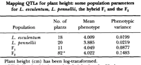
Mapping QTIs for plant height: some population parametea

for L. esculentum, L. pennellii, the hybrid F, and the F p

No. of Mean Phenotypic

Population plants phenotype variance

L. esculentum 18 4.009 0.0199

L. pennellii 20 3.885 0.0219

F, 1 1 4.049 0.0877

F* 82 a 4.022 0.1483

Plant height (cm) has been log-transformed.

RFLP data for 84 plants, plant height data for 82 plants.

model B, for the simultaneous effect of a single QTL and one marker, and so on. Many tests are performed when moving along the genetic map. An overall significance level cannot be guaranteed due to the current lack of knowledge about the statistical behavior of the (inter- dependent) tests. Using a significance level of 0.001 per test, the overall significance level in conventional inter- val mapping would be between 1

%

and 5% for a genome of 12 chromosomes covered with 50 markers

(KNom

and HALEY 1992). We use the same significance level per

test (0.001) in the practical example on tomato plants described in the next section, but an overall significance level for our mapping approach cannot be guaranteed. The chi-squared threshold at a significance level of 0.001

per test equals 13.8 for 2 d.f.; it is 16.3, 18.5, 20.5, 22.5, 24.3 and 26.1 for 3, 4, 5, 6, 7 and 8 d.f., respectively.

By

using a high significance level per test the probability of missing any existing QTL may become undesirably large. QTLs the presence of which cannot be demon- strated significantly may still partly explain the differ- ences for phenotypic values between the parents, F, and F,. Therefore, selected markers may be retained in the regression even though no QTLs are indicated signifi- cantly in the nearby region.

APPLICATION

A practical example on plant height in an

F,

progeny of tomato will be used to illustrate the methods de- scribed in the previous section; additional parental and F, data and marker cofactors are used in the interval mapping. The data are part of a larger experiment, the details and results of which will be reported elsewhere. The parents were a commercial tomato cultivar (Ly- copersicon esculentum) and a wild species (Lycopersicon Pennellii)

.

In the F, 52 restriction fragment length poly- morphism (RFLP) markers were scored. Plant height was measured six weeks after sowing. Mean phenotypic values and variances for the parents, the F, and the F,

progeny are presented in Table 2. A log-scale was used as is commonly done for young plants when growth is nearly exponential. Four percent of the marker data were missing. Two of the 84 F, plants had broken tops

SO that their observations of plant height were missing.

Nevertheless, their marker data could still be used for mapping markers.

The markers were assigned to linkage groups and mapped (and the recombination frequencies between adjacent markers were estimated) by using the com- puter package JoinMap (STAM 1993). The total number of markers is 52, so that the total number of parameters in the regression of the phenotype on all markers is equal to 104. This number exceeds the number of F, plants (82), and is still too large for reliable model se- lection even when parental and F, data are added (49

plants). Therefore, we applied the procedure of marker selection described above, using the F, data. These se- lected markers were subsequently used as cofactors in interval mapping (also some non-selected marker co- factors were added again during the interval mapping stage; see below). Next, the phenotypes of the F, prog- eny, the parents and the F, progeny were simultaneously regressed on a single QTL and on selected markers. This putative QTL was moved along the genetic maps of the various chromosomes. The results are shown in Figure

1. The impact of a single putative QTL on a given chro- mosome is indicated by the deviance between models A ,

(with QTL) and B, (without QTL); in both cases the selected markers on the other chromosomes were used as cofactors (finely dashed lines). The joint effect of the putative QTL and selected markers on the same chro- mosome is expressed by the deviance between models A ,

(with QTL and all selected markers) and B2 (without QTL, with selected markers on other chromosomes only) (coarsely dashed lines).

At least six QTLs were indicated, one on each of the chromosomes 6,

7,

8 and 9 (in the regions were the finely dashed lines in Figure 1 exceed the critical level of 16.3) and two QTLs on chromosome 2 (in the regions close to the marker cofactors; see below). Selected mark- ers on chromosomes 3, 5 and 10 were retained in the regression to absorb effects of possible QTLs whose pres- ence could not be demonstrated significantly, but which still explain a part of the phenotypic variation. On chro- mosome 8 the smallest AIC value of model A , is much less than the smallest AIC value of model A , (the AIC

difference is 41.93 - 27.96 -

2k

= 5.97

>

2, where k is the number of free parameters for the additional two co- factors; see Figure 1 ) . This indicates multiple QTLs on chromosome 8. However, the deviance difference of

13.97 is still not significant: it is less than the critical value of 18.5. We did present only the most apparent result (estimates for a single QTL on chromosome 8),

but we should bear in mind that the true genetic back- ground can be more complex (multiple QTLs on chromosome 8). On chromosome 2 the joint contri- bution of the two marker cofactors to the deviance is significant: the coarsely dashed line in Figure 1 ex- ceeds the critical value of 18.5. The effect of the co- factors are opposite, which indicates an extremely dif- ficult case to unravel: linked QTLs with opposite effects. The finely and coarsely dashed lines in Figure

1452 R. C. Jansen and P. Stam

!

CHROMOSOhlE 2

MI

I

50

bo.

bo.

n .

0

CHROMOSOME 7 CHROMOSOME 8

bo

-

-

" /

- -

"

Io

I

l"---l

cofactors, respectively. We also fitted model A, with either the first or the second cofactor; the estimates of the two QTLs are based on these models. The effect of one QTL is estimated on the assumption that the effect of the other QTL is eliminated by the marker cofactor.

Table 3 presents estimates of the QTL effects. Three out of the six QTLs have large positive additive effects, the other three have large negative additive effects. Note that the parents, the F, and the F, have approximately the same mean height (Table 2), so that the effects of the QTLs should approximately cancel. The discrepancy between the summed QTL effects and the observed dif-

"r

CHROMOSOME 9

m

CHROMOSOME 10

l

"

-

-

-

7

dl,

CHROMOSOME 12

M T I l w w l

FIGURE 1.-Deviance plots for plant height in an F, progeny of

tomato. The phenotypes of the F, progeny were regressed on a putative QTL, which was moved along the genetic map of each chromosome ("conventional" interval mapping). The deviance between the model with the QTL (model C) and the model without the QTL (model D ) was plotted (solid line). The phe- notypes of the F, progeny, the parents and the F, progeny were simultaneously regressed on a putative QTL and a number of

selected markers; again the QTL was moved along the genetic map. The finely dashed line shows the plot of the deviance be- tween model A, (with the QTL) and model B, (without the QTL); in both cases all selected markers from other chromo- somes were used. The coarsely dashed line represents the plot of the deviance between model A , (with the QTL and all selected marker cofactors) and model B2 (without the QTL but with se-

lected markers only on other chromosomes).

ferences between the parents could be due to undetec- ted QTLs; their effects are hopefully eliminated by the marker cofactors. The pooled environmental variance for the original parents and the F, equals 0.0273 (after removing one F, plant; see below). Table 3 shows that this value is approximated very well by using single QTL models with marker cofactors on other chromosomes, indicating that these models explain the total genetic variation satisfactorily.

High Resolution Interval Mapping 1453

TABLE 3

&timates of QTL effects, residual variance and recombination frequency between QTL and left flanking marker

Chromosome _{QTL effects}

(and marker Recombination

interval) Additive Dominance Variance frequency *

2 0.255 0.026 0.0197 0.130

2 -0.247 -0.071 0.0208 0.091

(4-) (0.043) (0.057) (0.0050) (0.040)

(1-2) (0.044) (0.063) (0.0043) (0.039)

7 -0.248 -0.114 0.0236 0.111

( 2-3) (0.050) (0.065) (0.0053) (0.041)

6 -0.204 0.205 0.0244 0.070

(2-3) (0.047) (0.067) (0.0043) (0.039)

8 0.272 0.118 0.0181 0.165

(1-2) (0.058) (0.064) (0.0028) (0.038)

9 0.249 -0.087 0.0249 0.111

(1-2) (0.037) (0.048) (0.0042) (0.036)

Standard errors of the estimates are presented between brackets.

The QTL was moved along the genetic map with steps of 2.5 cM; the recombination between the QTL and its left flanking marker is reported. deviance plot for chromosome 8 showed a clear peak,

indicating a QTL between marker 1 and

2.

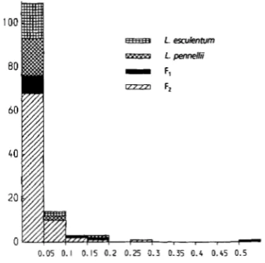
Therefore, the second time two cofactors were added on chromo- some 8 to eliminate the putative QTL effect. Next the weighted sums of squared residuals were checked for outliers. Figure 2 presents a histogram of the weighted sum of squared residuals obtained from the multiple linear regression of the phenotype of the F, progeny, the parents and the F, progeny on all selected markers. At a significance level of 0.01 the critical value equals a p proximately 0.24, so that one observation from the F, may be considered to be an extreme outlier. One plant of the F, progeny has a weighted sum of squared re- siduals just exceeding the critical value. The F2 outlier also caused narrow sharp peaks in the coarsely dashed lines close to marker cofactors (not shown): the factor for a putative QTL absorbed the effect of the outlier rather than an effect of a true QTL. The plant heights

of these two outliers were removed, which reduced the variance among F, plants from 0.0877 to 0.0512, and changed the variance among F, plants from 0.1483 to 0.1499 (see Table 2). For the third and final time the interval mapping was then passed through. After each successive passing of interval mapping the peaks shown in Figure 1 for chromosomes 6, 7,8 and 9 became more pronounced.

To compare the above results with conventional in- terval mapping, the phenotypes of the

82

F, plants were regressed on a single putative QTL, which was moved along the genetic map. The deviance between the model with the single QTL (model C ) and that without the single QTL (model

D )

was plotted at each map position (solid line in Figure 1 ) . A comparison of deviance curves for chromosomes 6,

7,

8 and 9 demonstrates that our approach is much more powerful than conventional in- terval mapping. Only two QTLs are detected by con- ventional interval mapping (one QTL on chromosome

100

-

L. esculenhm

m 1. pennellii

-

4

-

F,

80

0.05 0.1 0.15 0.2 0.25 0.3 0.55 0 . 4 0.45 0.5

FIGURE 2.-Histogram of the weighted sum of squared re- siduals, used for the detection of outliers for plant height in an F,progeny of tomato. The residuals were obtained from the mulhple linear regression of the phenotypes of the F, progeny,

the parents and the F, progeny on all selected markers. Two outliers are indicated, namely the plants with the weighted

sum of squared residuals >0.24.

6 and one on chromosome

7).

DISCUSSION

1454 R. C. Jansen and P. Stam

at directly; nevertheless, the example given illustrates the potential contribution of our new analytical method to progress in these areas. The phenotypic variation of the quantitative trait was resolved into at least six puta- tive QTLs and an environmental error component. These results should still be regarded as preliminary; they have to be confirmed by further experiments. Fa lines, isogenic for regions of putative QTLs, may be pro- duced and tested (PATERSON et al. 1991); also backcross inbred lines may be used for this purpose (BECKMANN and SOLLER 1989).

Our approach to QTL mapping uses the unified con- cept of completing missing genotypic data for both a putative QTL and markers. If many data are missing, this may give rise to computational problems: in an

F,

one missing marker observation may actually have one of three allelic constitutions, two missing marker observa- tions (for the same plant) result in nine possible con- stitutions, and so on. If in a data set with many markers a certain proportion of the marker genotypes is missing, the number of weighted completed data may become so large that computation is no longer feasible. Molecular geneticists, who are generally collecting the marker data, should be aware of the consequences of missing marker data, so that they hopefully will strive for com- pleteness of their data. However, to complete data it is not necessary to use all available information; the amount of computation can be reduced considerably by a limited completion of missing data: genotypes with negligible weights may be disregarded, without substan- tial loss of information.

In conventional interval mapping data from the par- ents and the F, progeny cannot be used; if the parental and F, data were included, the results would be seriously biased because the single QTL would be called upon to explain all the mean differences between the parents and the

F,

progeny. It is only because markers are used as cofactors in our approach that data from parents and F, can be included; QTL mapping may become much more powerful when marker cofactors explain a large proportion of the genetic variation (or at least the mean difference between the parents and the F, progeny). In other cases, for instance when there are numerous QTLs of small effect distributed throughout the genome, the power of QTL mapping may be reduced by using pa- rental and F, data, because the additional constraints on the parameters are too exacting.

In our example data set, an interaction between marker cofactors and a putative QTL is indicated (Fig- ure 1, chromosome 8): if the inclusion of marker CO-

factors simply reduced the residual variance, the solid and finely dashed lines should be approximately similar in shape, although the finely dashed lines might be higher. We speculate that in the small F, progeny of 84 plants in our example, deviant segregation ratios for two or more unlinked QTLs have masked the effect of the

QTL on chromosome

8

when we applied the conven- tional interval mapping method. In our approach, the effects of the QTLs involved could be unraveled by the use of marker cofactors. This problem for small popu- lations should be explored in more detail by simulation. Little is known about the influence of outliers on QTL mapping; we proposed a weighted sum of squared re- siduals to indicate outliers. Two particular observations in the example data set were detected as potential out- liers. It was observed that such outliers can incorrectly indicate multiple linked QTLs. Also they may hamper efficient and accurate resolvability of QTLs.

In the example we have come across a situation which represents a “worst case” configuration: linked QTLs with opposite effects.

As

indicated by

STAM

(1991), and confirmed by the present study, in such a case multiple regression will be more powerful than “conventional” interval mapping. Our single data set cannot answer the general question as to what resolution power is attain- able with our method. To answer this question a number of known configurations of QTLs and QTL effects, as well as heritability and population size, need to be stud- ied by simulation.

The regression models that are used in our ap- proach assume additivity of effects over loci. Though epistatic effects can in principle be modeled straight- forwardly as well, we have chosen not to do so because of the rapid increase of the number of parameters, relative to the amount of data. In our view, however, the detection of epistatic effects requires a different type of experimental approach, such as raising the F, offspring of deliberately chosen F, multilocus marker genotypes.

The authors are greatly indebted to P. ODINOT and W. H. LINDHOUT, Department of Vegetables and Fruit Crops of CPRO-DLO, for s u p plying the data of the example.

LITERATURE CITED

BECKMANN, J. S., and M. SOUR, 1989 Backcross inbred lines for map ping and cloning of loci of interest, pp. 117-122 in Development

and Application of Molecular Markers to Problems in Plant Ge-

netics, edited by B. BumandT. HELENTJARIS. Brookhaven National

Laboratory.

GENSTAT 5 COMMI’ITEE, 1987 Genstat 5 Reference Manual. Clarendon Press, Oxford.

H A L E Y , C. S., and S. A. &om, 1992 A simple method for mapping quantitative trait loci in line crosses using flanking markers. Heredity 6 9 315-324.

JANSEN, R. C., 1992 A general mixture model for mapping quanti- tative trait loci by using molecular markers. Theor. Appl. Genet.

JANSEN, R. C., 1993a Maximum likelihood in a generalized linear fi- nite mixture model by using the EM algorithm. Biometrics 49:

JANSEN, R. C., 1993b Interval mapping of multiple quantitative trait loci. Genetics 135: 205-211.

KNAPP, S. J., 1991 Using molecular markers to map multiple quan-

titative trait loci: models for backcross, recombinant inbred, and doubled haploid progeny. Theor. Appl. Genet. 81:

333-338.

85: 252-260.

High Resolution Interval Mapping 1455

KNOIT, S. A., and C. S. HALEY, 1992 Aspects of maximum likelihood methods for the mapping of quantitative trait loci in line crosses. Genet. Res. 60: 139-151.

LANDER, E. S., and D. BOTSTEIN, 1989 Mapping Mendelian factors underlying quantitative traits using RFLP linkage maps. Genetics

121: 185-199.

MCCULLAGH, P., and J. A. NELDER, 1989 Generalized linear models, in

Monographs on Statistics and Applied Probability 37. Chapman

& Hall, London.

PATERSON, A. H., E. S. LANDER, J. D. HEW, S. PETERSON, S. E. LINCOLN

et al., 1988 Resolution of quantitative traits into Mendelian fac-

tors by using a complete linkage map of restriction fragment poly- morphisms. Nature 335: 721-726.

PATERSON, A. H., S. D. DAMON, J. D. HEW, D. W I R , H. D. RABINOWTCH

et al., 1991 Mendelian factors underlying quantitative traits in

tomato: comparison across species, generations and environ- ments. Genetics 127: 181-197.

SAKAMOTO, Y., M. ISHIGURO and G . KITAGAWA, 1986 Akaike Information

Criterion Statistics. KTK Scientific Publishers, Tokyo.

STAM, P., 1991 Some aspects of QTL mapping, in Proceedings of the

Eighth Meeting of the Eucarpia Section Biometrics in Plant Breed-

ing. Brno, July 1991.

STAM, P., 1993 Constructing integrated genetic linkage maps by means of a new computer package: JoinMap. Plant J. 3:

739-744.

STLJBER, C. W., S. E. LINCOLN, D. W. WOLFF, T. HELENTJARIS and E. S.

LANDER, 1992 Identification of genetic factors contributing to heterosis in a hybrid from two elite maize inbred lines using mo- lecular markers. Genetics 132: 823-839.

VAN OOIJEN, J. W., 1992 Accuracy of mapping quantitative trait loci in autogamous species. Theor. Appl. Genet. 84: 803-811. WELLER, J. I., 1986 Maximum likelihood techniques for the mapping

and analysis of quantitative trait loci with the aid of genetic mark- ers. Biometrics 4 2 627-640.

Communicating editor: W. G . HILL

APPENDIX

Updating the estimates of the recombination frequen- cies in the EM algorithm runs parallel to the “normal”

EM procedure for estimation of T from F, data, as out-

lined below. In an F, recombinant the F, gametes could be counted directly from the frequencies of the geno- types AA, AH, AB, HA, HH, HB, BA, BH and BB if the contribution of repulsion and coupling phase to HH

were known. Given the current estimate, r, the ratio of repulsion and coupling phase within the double het- erozygotes equals r2: (1 - T ) ‘ . Denoting the observed

genotypic frequencies by n ( A A ) , n ( A H ) , etc., the EM

procedure runs as follows:

E

step: Update the unknown number of repulsion heterozygotes.

M step: Obtain the new estimate by counting recom- binant gametes.

This leads to the following update

n(AH)

+

n(HA)

+

n(BH)

+

n(HB)

+

2{n(AB)

+ n(BA)

+

[ r P / ( r p

+

(1 - r)‘] * n(HH)} i =

2

1

4 . 1

When updating the estimate of r in our QTL mapping method, the above equation is used; the numbers n(*)

are replaced by the updated summed weights w ( * ) ,