ABSTRACT
NIE, TIANTIAN. Quadratic Programming with Discrete Variables. (Under the direction of Dr. Shu-Cherng Fang.)
Quadratic Programming with Discrete Variables
by Tiantian Nie
A dissertation submitted to the Graduate Faculty of North Carolina State University
in partial fulfillment of the requirements for the Degree of
Doctor of Philosophy
Industrial Engineering
Raleigh, North Carolina 2016
APPROVED BY:
Dr. James R. Wilson Dr. Yunan Liu
Dr. Osman Ozaltin Dr. Shu-Cherng Fang
DEDICATION
Dedicated to
BIOGRAPHY
ACKNOWLEDGEMENTS
I would like to express my deepest and sincerest gratitude to my advisor Dr. Shu-Cherng Fang for his great guidance, support and encouragement through my Ph.D. study. He not only supervises me on conducting good research, but also sets a perfect example for me to be a rigorous scholar, kindly teacher and wise person. More importantly, he is like a father encouraging me to enjoy life and live happily.
I am also very grateful to my committee members - Dr. James R. Wilson, Dr. Yunan Liu and Dr. Osman Ozaltin for their valuable comments and suggestions on my research and presentation. Their encouragement inspired me to excel in my work and be more confident. Thanks also go to the graduate school representative Dr. Min Liu for her generous support and help. I would also like to thank Dr. John E. Lavery for his kindly help in my Ph.D. study and his strong mind that inspired me a lot.
I want to thank Mr. Edward Fitts for the Edward P. Fitts Fellowship that supports my graduate study. Also I am grateful to the staff of the Industrial and Systems Engineering Department, especially Ms. Cecilia Chen, Mr. William Irwin, Mr. Justin Lancaster and Mr. Robert Lasson, for their support and help during my graduate study.
I am really lucky to receive the support and encouragement from all my fellow friends in the FANGroup and the ISE Department: Ye Tian, Zhibin Deng, Jian Luo, Ziteng Wang, Chien-Chia Huang, Jiahua Zhang, Giyoung Kim, Yao Yu, Sha Luo, Qi An, Ling Zhang, Yu-Liang Lin, Chi-Yi Chen, Shan Jiang and so many others that I cannot list them all. In particular, I would like to thank Zhibin Deng for his guidance on my graduate study. Sincere thanks also go to my dear friends Yicong Yong, Eileen Gu and all roommates in apartment 101 for their friendship that made my life sweet in Raleigh.
TABLE OF CONTENTS
List of Tables . . . vii
List of Figures . . . .viii
Chapter 1 Introduction . . . 1
1.1 Problem Statement and Motivation . . . 1
1.2 Contributions . . . 3
1.3 Outline of the Dissertation . . . 6
Chapter 2 Literature Review and Basic Knowledge . . . 7
2.1 Notation . . . 7
2.2 Quadratic Programming with Discrete Variables . . . 8
2.2.1 Relaxation Approach . . . 8
2.2.2 Reformulation Techniques . . . 9
2.2.3 Branch-and-Bound Algorithms . . . 10
2.3 Quadratic Programming and Linear Conic Optimization . . . 11
Chapter 3 A Linear Conic Relaxation Approach . . . 16
3.1 Introduction . . . 16
3.2 A new linear conic relaxation problem . . . 18
3.3 Special structure and properties . . . 21
3.4 Effectiveness and robustness of lower bounds . . . 27
3.5 Extensions to constrained DQP problems . . . 30
3.6 Summary . . . 32
Chapter 4 A Linearization Method. . . 34
4.1 Introduction . . . 34
4.2 Proposed Super Logarithmic Method . . . 38
4.3 Comparison with other methods . . . 44
4.4.1 General product term . . . 45
4.4.2 Fractional term . . . 48
4.4.3 Representable programming problems . . . 49
4.5 Numerical experiments . . . 50
4.5.1 Compression spring design optimization problem . . . 50
4.5.2 Pressure vessel optimization problem . . . 52
4.5.3 Speed reducer design problem . . . 53
4.6 Linearization of DQP . . . 55
4.6.1 A single discrete-valued quadratic term . . . 55
4.6.2 DQP with multiple discrete-valued quadratic terms . . . 56
4.6.3 Enhancement . . . 57
4.7 Summary . . . 61
Chapter 5 l1-norm Constrained Convex Quadratic Programming with Dis-crete Variables. . . 63
5.1 Introduction . . . 63
5.2 Preliminaries . . . 65
5.2.1 Basic properties ofl1-norm constraints . . . 65
5.2.2 Mixed-integer conic rounding cuts . . . 66
5.3 Conic Cuts of (l1-DQP) . . . 68
5.3.1 Conventional SOC cuts . . . 68
5.3.2 New conic cuts . . . 69
5.3.3 Analysis of conic aggregation strategy . . . 71
5.4 Numerical Experiments and Results . . . 73
5.4.1 Partial conic aggregation procedure . . . 74
5.4.2 Numerical results . . . 75
5.5 Summary . . . 81
Chapter 6 Conclusions. . . 82
6.1 Summary and Contributions . . . 82
6.2 Future Research . . . 84
LIST OF TABLES
Table 3.1 (DQP) with convex quadratic objective function . . . 28
Table 3.2 (DQP) with non-convex quadratic objective function . . . 28
Table 3.3 Computational timet2 (seconds) of solving (LCoR2) . . . 29
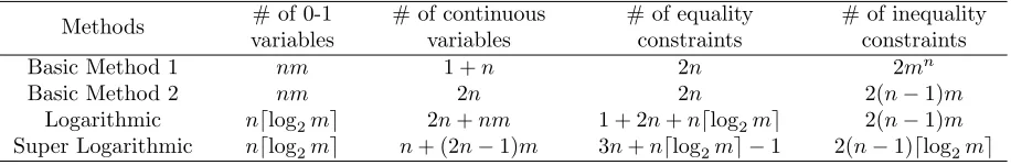
Table 4.1 Comparison of four methods for linearizing one signomial term . . . 45
Table 4.2 Experimental results of compression spring design optimization problem . 52 Table 4.3 Experimental results of compression spring design optimization problem . 53 Table 4.4 Experimental results of compression spring design optimization problem . 54 Table 4.5 Comparison of three methods for linearizing one quadratic term . . . 56
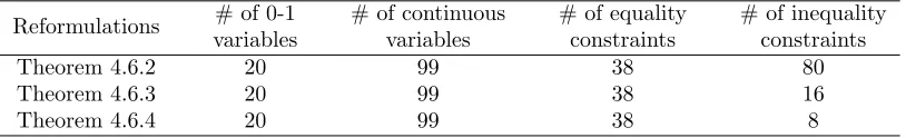
Table 4.6 Comparison of three SLM based reformulations of DQP example . . . 61
Table 5.1 Computational results (average), n= 40, m= 40, u= 1 . . . 76
Table 5.2 Outcome percentage of the 200 instances . . . 78
Table 5.3 Computational results of Type-II instances (average) . . . 79
LIST OF FIGURES
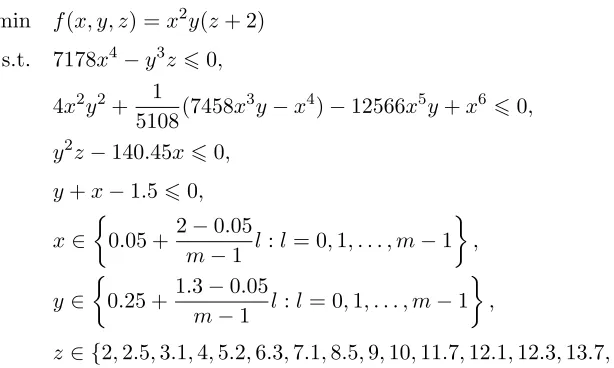
Figure 4.1 Compression spring design optimization problem . . . 51
Figure 4.2 Tube and end section of pressure vessel . . . 53
Figure 4.3 Speed reducer . . . 54
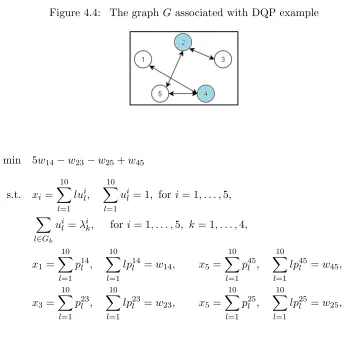
Figure 4.4 The graph Gassociated with DQP example . . . 60
Figure 5.1 Simple conic rounding cut for |x−b| ≤t . . . 68
Figure 5.2 Conic inequalities based on various 0-1 multipliers . . . 72
Figure 5.3 Impact of adding conic cuts, n= 40, m= 40, u= 1 . . . 77
Figure 5.4 Impact of adding comprehensive conic cuts, u= 5 . . . 79
Chapter 1
Introduction
Quadratic programming with discrete variables (DQP) is an important nonlinear discrete op-timization problem. Motivated by the progress made in quadratic programming and integer programming, DQP has recently moved into the focus of optimization research. The aim of this dissertation is to investigate more effective solution methods for DQP by exploiting its special structure and utilizing the advanced continuous optimization techniques.
1.1
Problem Statement and Motivation
A quadratic programming problem with discrete variables is a mathematical optimization prob-lem in which each variable is restricted to a finite set of discrete values and the objective function is quadratic. DQP can be written in the following form:
min 12xTAx+cTx
s.t. xi∈ {di1, . . . , dimi}, i= 1, . . . , n,
(1.1)
whereA∈ Snis a symmetric matrix,c∈
Rnis a cost vector andx∈Rnis the vector of decision variables in whichxi may takemi possible values of{di1, di2, . . . , dimi}withd
i
1 < di2 < . . . < dimi, for i = 1, . . . , n. Without loss of generality, we may assume that di
1 > 0 and m1 = m2 =
. . .=mn. But our work is also applicable to the general case with somedi1 <0 andmi 6=mj,
i, j∈ {1, . . . , n} and i6=j.
equivalent DQP problem. Other applications include the closest vector problem in communi-cation systems [57], optimal design in process systems engineering [11] and resource allocommuni-cation in distributed computing systems [28]. DQP also has great importance for theoretical research in discrete optimization. The well-known max-cut problem [65], binary quadratic programming problem [84] and ternary quadratic programming problem [63] are special cases of DQP, with xi ∈ {−1,1}, xi ∈ {0,1} and xi ∈ {−1,0,1}, for i = 1, . . . , n, respectively. So is the integer
quadratic programming problem [56], with xi ∈Z∩[li, ui] and li 6ui fori= 1, . . . , n, which
has recently attracted lots of attention.
It is known that DQP is nondeterministic polynomial-time hard (NP-hard) in general [58, 62], even for the simple version of binary quadratic programming. With integer variables, linear programming problems have been extensively studied for many decades [70], while practical methods for the nonlinear case, even when the objective is quadratic, are still rare and ineffective [36]. Moreover, since DQP requires variables to be of general discrete values, known methods of integer quadratic programming may not be directly applicable for solving DQP.
Since it is hard to find exact solutions to DQP (due to the NP-hardness), one may compro-mise to consider high-quality approximate solutions that can be obtained in polynomial time. In practice, heuristic techniques search for good candidate solutions, however, they are restricted to specific subclasses of DQP with special structures [23]. From a global optimization point of view, the task is to explore tight and polynomial-time solvable approximations for DQP. Along this direction, both the discreteness and non-convexity of the problem need to be treated. In the literature, approximations of DQP have been studied but mainly for the subclass of 0-1 binary quadratic programs (BQP) [30, 55, 56, 84]. Note that the 0-1 binary requirement of variables is equivalent to a set of quadratic equality constraints, hence BQP also belongs to the class of continuous quadratic programming problems (QP). The difficulty in developing approximations for BQP is then reduced to handling the non-convexity only. The embedded continuous nature of BQP also enables researchers to investigate high-quality approximations of BQP following those of QP, which have been extensively studied using advanced continuous op-timization techniques in recent decades. When it comes to DQP with general discrete variables, effective approximate solutions methods that handle both the discreteness and non-convexity of DQP are still missing.
system-atic manner. For finding exact solutions, the efficiency of a branch-and-bound scheme is then impacted by both the complexity of the branching tree and the computational cost at each branching node. A tighter bounding routine may reduce the number of nodes explored, but at the same time imply heavier computational burden of node checking. Hence, A trade-off exist between the computational efficiency and quality of the lower bound obtained for branching. In the literature, we have seen extensive studies on the branch-and-bound schemes of classical mixed-integer linear programming problems (MILP). The scheme branches according to the integer requirement of variables and solves continuous relaxation problems to provide lower bounds for branching. In the meanwhile, an advanced technique that incorporates valid linear inequalities induced by the integer requirement (called as “mixed-integer linear cut”) is usually applied for improving the overall computational efficiency of the branch-and-bound scheme.
For our problem DQP, a sublass of nonlinear discrete optimization, branch-and-bound based exact solution methods can be explored in two main directions. On one hand, since efficient branch-and-bound based commercial MILP solvers are available, it remains to develop effective MILP representations for DQP. In fact, for a continuous nonlinear program, the equivalent linear representation does not exist in general. It is the discrete nature of DQP that enables us to reconstruct the nonlinear feature of DQP in a linear manner. Therefore, exploiting the nonlinear feature’s discrete property may help us design effective MILP reformulations for DQP. The other exact solution method is to develop efficient branch-and-bound algorithms for DQP with specific branching rules and bounding routines. Intuitively, one may branch according to the discrete requirement of variables and then solve convex continuous relaxation problems for providing lower bounds at branching nodes. Some convex-relaxation-based branch-and-bound algorithms of DQP can be found in [18, 19, 20]. In the meanwhile, the conventional linear cut generation method does not apply here since DQP is a nonlinear problem. But in the special case when DQP has a convex objective function, we have seen some preliminary theoretical research on the mixed-integer nonlinear cuts in the recent literature [7, 8].
From the above mentioned, we may see that the study of DQP is an emerging research area yet effective solution methods of DQP are less studied. In particular, the discrete, nonlinear and non-convex properties have not been fully exploited in current solution methods of DQP. In this dissertation, we intend to explore more effective solution methods for DQP by exploiting its special structure and utilizing state-of-the-art continuous optimization techniques.
1.2
Contributions
A linear conic programming (LCoP) problem minimizes a linear function over the inter-section of an affine subspace and a convex cone, which may involve special structures such that the LCoP problem can be solved in polynomial time. The advanced linear conic relaxation approach was initiated for continuous quadratic programming problems (QP). It packs all difficulties of QP into a convex cone in a higher dimensional matrix-space and then relaxes the convex cone to a well-structured one. In this way, a polynomial-time solvable LCoP relaxation problem is constructed. Several linear conic relaxations for QP have been shown to be tight for providing high-quality lower bounds [16, 22, 54, 56]. We adopt the linear conic relaxation approach to propose a special linear conic relaxation for DQP, based on a linearly constrained 0-1 binary quadratic programming reformulation of DQP. Numerical results verify that the proposed linear conic relaxation is capable of providing high-quality and robust lower bounds for DQP. Moreover, we find that the discrete nature of DQP brings a special property to the proposed linear conic relaxation. The optimal solution of the proposed relaxation problem is in the form of a matrix, whose rank is defined as the size of the largest collection of linearly independent columns. We have shown that when the proposed relaxation problem has an optimal solution with rank one or two, optimal solutions to the original problem DQP can be explicitly generated. This special property can be further extended to the linear conic relaxations of DQP with linear constraints. The results of this part of work have been published in [60].
(2) A new linearization method has been developed.
For the purpose of finding exact solutions to DQP, we fully exploit the discrete structure embedded in the discrete quadratic terms to develop effective 0-1 MILP reformulations for DQP. Note that the quadratic feature can be generalized to the product of multi-ple variables. We first investigate the linearization of the following generalized signomial programming problem with discrete variables (DSP):
min PJ
j=1
cj n
Q
i=1
(xi)ai,j
s.t. xi∈ {di1, . . . , dim}, i= 1, . . . , n,
inequality constraints and binary variables. Both the theoretical analysis and numerical results strongly support its superior performance when compared with known state-of-the-art linearization methods. Later, we customize the proposed method to provide effective 0-1 MILP reformulations for DQP. In particular, for DQP with special network-structured coefficients, the reformulation of DQP can be further enhanced for better efficiency. The results of this work can be found in a published paper [45].
(3) A variation of DQP withl1-norm constraints has been explored.
We further extend our study to a special linearly constrained DQP problem, called l1 -norm constrained convex quadratic programming with integer variables (l1-DQP), which
is commonly seen in real-life applications due to the favorable sparse and outlier-robust properties of thel1-norm. While the solution concepts of DQP are naturally applicable to l1-DQP, here we explore the special conic structure of thel1-norm to investigate advanced
solution methods for l1-DQP.
Due to the convexity of the quadratic objective function, second-order conic (SOC) cuts induced from the integer requirement are usually adopted in solvingl1-DQP by a branch-and-bound scheme [7, 8, 24]. By exploiting the first-order conic structure embedded in the l1-norm constraint, we develop new ways to generate and manage conic cuts of l1-DQP.
Numerical results show that the proposed conic cuts work more effectively than the SOC conic cuts in reducing the complexity of branching trees and improving the computational efficiency of the branch-and-bound scheme. The results of this work have been documented in a working paper [61].
1.3
Outline of the Dissertation
Chapter 2
Literature Review and Basic
Knowledge
In this chapter, we review the related studies of DQP and some preliminary knowledge. Some useful notations are first introduced in Section 2.1. In Section 2.2, a literature review of DQP is presented, while some basic knowledge about the relation between quadratic programming and linear conic optimization is given in Section 2.3.
2.1
Notation
We denote the set of real numbers and nonnegative real numbers by R and R+,
respec-tively. In the n-dimensional real space Rn, let the set of nonnegative real vectors be Rn+.
Denote the set of nonnegative integer numbers and the set of nonnegative integer vectors in Rn by Z+ and Zn+, respectively. The lp norm of a vector x ∈ Rn is given by kxkp =
(Pn
i=1|xi|p) 1/p
, for p ∈ Z+ and the corresponding n-dimensional pth-order cone is defined as
n
x∈Rn| (|x1|p+. . .+|xn−1|p)1/p≤xn
o
. In particular, the n-dimensional second-order cone is denoted byLn.
LetRm×nbe the set ofm×nreal matrices,Snbe the set ofn×nsymmetric real matrices, Sn
+ = {A ∈ Sn : A < 0} be the set of n×n positive semidefinite matrices, Nn = {A ∈
Sn :A ≥ 0} be the set of n×n entry-wise nonnegative matrices. The set Sn
+∩ Nn is called
a doubly nonnegative cone. For a matrix A ∈ Sn, A
ij stands for the element in the i-th row
and j-th column of A. Let 1m×n and 0m×n bem×n matrices with all entries equal to 1 and
0, respectively, and In be a diagonaln×nmatrix with all diagonal entries equal to 1. The dot
product operation in Rm×n is given byA•B= trace(ABT).
that contains F. Whereas, the conic hull of F defined as the smallest convex cone containing F is denoted by cone{F }. Given two sets A and B, let A\B denote the relative complement of Awith respect to B, i.e., the set of elements inA but not inB.
2.2
Quadratic Programming with Discrete Variables
As a commonly seen practical model in engineering design and system sciences, DQP was primarily studied using heuristic techniques such as simulated annealing [6] and genetic algo-rithms [50]. These heuristic techniques find some candidate solutions that may be close to an optimal one for DQP. In addition, some effective relaxation and reformulation techniques and branch-and-bound methods have been developed for finding solutions to DQP.
2.2.1 Relaxation Approach
Relaxations of DQP construct polynomial-time solvable problems that provide approximate so-lutions and high-quality lower bounds for DQP. In the literature, most relaxations of DQP considered the special case when the discrete variables are binary, in particular, a 0-1 bi-nary quadratic programming problem (BQP). Linear conic relaxation was originally applied to quadratic programming with continuous variables (QP) which includes BQP as a special case. We will review the relationship between linear conic programming (LCoP) and QP in Section 2.3.
However, research on the relaxations of the general DQP problem can hardly be found except [20], which was motivated by the observation that DQP can be modeled as an SDP plus a rank-one constraint. Embedded in a branch-and-bound framework of DQP, this SDP relaxation was not designed for providing high-quality approximate solutions and lower bounds for DQP.
2.2.2 Reformulation Techniques
Although good commercial solvers can directly handle nonconvex mixed integer programming problems, the computation may still be inefficient. In order to improve the computational efficiency, an effective representation of DQP is desired for fast computation.
An initial step of reformulating DQP linearly expresses the discrete variables. For a discrete variable xi ∈ {di1, . . . , dimi}, a naive linearization method is to introduce new binary variables ul ∈ {0,1}, l = 1, . . . , mi, satisfying u1 +u2 +. . .+umi = 1 such that xi can be linearly represented asxi=di1u1+di2u2+. . .+dimiumi. In practice, however, this linearization method would require a huge number of binary variables, which significantly limits the computational efficiency of a branch-and-bound-based solver. Recently, a logarithmic method is developed that requires a half order fewer binary variables to linearly represent a discrete variable, at the cost of introducing more continuous variables and linear constraints [12, 46, 89]. Numerical results showed that the logarithmic method is superior to other linearization methods in terms of the computational efficiency. With discrete variables linearly expressed, reformulation techniques of DQP fall into two main categories.
One is linearizing DQP as a 0-1 mixed integer linear programming problem. The main issue arises from the linearization of quadratic product terms with discrete variables [12, 72]. Expressing the discrete variables by 0-1 binary variables, it suffices to linearize the corresponding 0-1 quadratic programming problem. A most widely used technique of linearizing a quadratic termxywithx, y∈ {0,1}is the RLT method [73, 74, 77, 78], which introduces a binary variable z∈ {0,1} satisfying z6x, z6y andz>x+y−1 to represent the nonlinear termxy.
The other linearization technique is reformulating DQP as a 0-1 mixed integer convex pro-gramming problem. Different from the linearization technique, the quadratic convex reformu-lation (QCR) method is simply realized by adding a parameterized perturbation. For instance, consider the nonconvex quadratic function f(x) = xTAx+cTx with variables x ∈ F ⊆ Rn
and coefficients A ∈ Sn and c ∈
Rn. As long as the parameter λ satisfies A−λIn < 0, the
perturbed function ¯f(x;λ),f(x) +λPn
i=1(vi−x2i) becomes a convex quadratic function with
¯
f(x;λ) =f(x) under the condition ofvi =x2i, i= 1, . . . , n. However, to find a good parameterλ
term. This leads to various 0-1 mixed integer convex quadratic reformulations [13, 14]. 2.2.3 Branch-and-Bound Algorithms
Given a representation of DQP, branch-and-bound algorithms develop specific routines of branching and bounding that may significantly improve the computational efficiency of finding exact solutions to DQP. Most branch-and-bound algorithms face a trade-off between the quality of solution and computational time of bounding.
In [91], the canonical duality conditions of DQP were analytically derived for designing an effective branching routine for branch-and-bound. Recently, Buchheim et al. [18, 19, 20] pro-posed three different relaxation-based branch-and-bound algorithms for DQP. In [18], a special case of DQP, when the quadratic objective function is convex, was studied. They showed in this case the continuous relaxation of DQP can be easily solved during the branching process and valid cuts can be effectively generated to tighten the bounds. However, this bounding method is inapplicable to nonconvex DQP since the corresponding continuous relaxation can be NP-hard. Subsequently, they proposed a new nonconvex relaxation method [19]. Their nonconvex relax-ation is in the form of a trust region problem, which is an important nonlinear optimizrelax-ation problem with many efficient algorithms available [66]. In these two branch-and-bound algo-rithms [18, 19], lower bounds are provided by continuous relaxations of DQP. Differently, an SDP relaxation of DQP was given by [20], based on which a branch-and-bound algorithm was subsequently designed. The computational results in [18, 19, 20] showed that the SDP-based branch-and-bound algorithm is more efficient for solving DQP with many discrete values for each variable, while less efficient than the other two algorithms when the discrete variables become binary or ternary.
Under the branch-and-bound scheme of DQP, an advanced technique that has recently attracted a lot attention is developing effective nonlinear cuts induced from the discrete re-quirement, which can then be incorporated into branch-and-bound algorithms to tighten the continuous relaxations at branching nodes. This direction can be viewed as an extension of uti-lizing mixed-integer linear cuts in solving mixed-integer linear programming problems (MILP). However, due to the nonlinear property of DQP, the conventional linear cuts do not apply here. Alternatively, the progress was made in developing nonlinear conic cuts of mixed-integer order cone programming problems (MISOCP), an extension of MILP with second-order cone constraints involved. Note that an n-dimensional second-order cone Ln is given
by Ln = {x ∈
Rn|
q
x21+. . .+x2n−1 ≤ xn}. When DQP has a convex quadratic objective
function and integer variables, an equivalent MISOCP reformulation of DQP exists. Therefore, we may obtain corresponding mixed-integer nonlinear cuts of DQP.
representation of an original SOC constraint. In the meanwhile, disjunctive conic inequalities for representing the convex hull of a disjunctive conic set are also generated as conic cuts [8]. It is notable that the theoretical research on nonlinear conic cuts has not yet been extensively studied, not to mention the performance in numerical implementations. However, with the development of commercial solvers using linear conic programming based branch-and-bound algorithms, it shall be important to explore effective conic cuts with both theoretical and numerical support.
2.3
Quadratic Programming and Linear Conic Optimization
A convex set F ⊆Rm×n is a subset of
Rm×n such that
λX1+ (1−λ)X2∈ F, for any X1,X2∈ F and λ∈[0,1]. A coneC ⊆Rm×n is a subset of
Rm×n such that
λX ∈ C, for allX ∈ C and λ≥0. IfC further satisfies that
“X ∈ C and −X ∈ C” if and only if “X = 0”,
then we call it a pointed cone. C is called a solid cone if it has a nonempty interior. If C is pointed, solid, closed and convex, then we sayC is aproper cone.
Given a set F ⊆Rm×n, theconvex hulland conic hull ofF are expressed as
conv{F }=
X ∈Rm×n
X =
r
X
i=1
αiXi, r
X
i=1
αi = 1,Xi ∈ F,0≤αi≤1,
for somer ∈N andi= 1, . . . , r
and
cone{F }=
(
X ∈Rm×n
X =
r
X
i=1
αixi,Xi∈ F, αi≥0, for somer∈N and i= 1, . . . , r
)
,
respectively, which directly implies
A linear conic programming (LCoP) problem in the matrix space Rm×n is defined by
(LCoP)
min C•X
s.t. Ai•X =bi, i= 1, . . . , I,
X ∈ C,
where C is a closed convex cone and the notation “•” is the dot product. When m = 1 or n = 1, (LCoP) degenerates to a linear conic programming problem in the vector space. Lin-ear programming (LP) problems and positive semidefinite programming (SDP) problems are two commonly seen subclasses of the LCoP problem, with the cone C defined as Rn+ and S+n,
respectively. Both of Rn+ and S+n are proper cones and the corresponding LCoP problems are
polynomial-time solvable. When the coneC is defined ascl{cone{F }}for an arbitrary setF, the corresponding LCoP problem is in general NP-hard.
It is not hard to construct an equivalent linear conic programming reformulation for a quadratic optimization problem. Consider the following quadratic programming problem:
(Q) min
1
2xTAx+cTx
s.t. x∈ F,
where∅ 6=F ⊆Rnis a feasible domain, convex or not. We first transform (Q) into the following
form:
(QT)
min 12 0 c
T
c A
!
•V
s.t. V = 1
x
!
1 x
!T
, x∈ F.
Note that the objective function of (QT) is linear in terms of V. Hence, the optimal value of (QT) can be achieved on the boundary of the closure of the convex hull of its feasible domain. The closure of the convex hull of the feasible domain of (QT) is defined as
cl conv 1 x ! 1 x !T
x∈ F
.
problem:
(QLCoP) min
1 2
0 cT c A
!
•V
s.t. V11= 1, V ∈ D∗(F),
where the closed convex cone D∗(F) is defined as
cl cone 1 x ! 1 x !T
x∈ F
.
Therefore, the quadratic programming problem (Q) and linear conic programming problem (QLCoP) are equivalent.
However, reformulating a general nonconvex problem (Q) into a linear conic programming problem (QLCoP) does not make it easier to solve. All the implicit “difficulties” implied from the original feasible domain F are packed into the cone D∗(F). In [83], Sturm and Zhang
theoretically derived the representability ofD∗(F) for a special feasible domainF. Specifically, if F is defined by one quadratic constraint and one linear constraint, then the cone D∗(F) can be represented by linear matrix inequalities (LMI) over the positive semidefinite cone, which indirectly proved that the original problem (Q) is not NP-hard. However, in a general quadratically constrained case, as long as the original problem (Q) is NP-hard, the linear conic reformulation (QLCoP) cannot be solved in polynomial time. Then, we may want to relax the “difficult” cone D∗(F) to a polynomial-time detectable cone such that lower bounds of the original problem can be efficiently obtained. Effective relaxations depend on carefully exploring special structures of the coneD∗(F) [16, 56, 65, 84, 93].
The well-known SDP relaxation is a special subclass of linear conic relaxation for quadratic programming problems with linear and quadratic constraints [55, 81]. In particular, consider the following binary quadratic programming problem:
(BQP) min
1 2x
TAx+cTx
s.t. x∈ {0,1}n.
Note that problem (BQP) is equivalent to the following reformulated problem:
min 1
2
0 cT c A
!
•V
V = 1 x
T
x X
!
∈ Sn+1
+ , (2.2)
rank(V) = 1. (2.3)
The traditional SDP relaxation of (BQP) is derived as below by deleting the nonconvex con-straint, i.e., the rank-one constraint (2.3).
min 12 0 c
T
c A
!
•V
s.t. Xii=xi, i= 1, . . . , n,
V = 1 x
T
x X
!
∈ S+n+1.
The SDP relaxation of (BQP) can actually be regarded as a relaxation of the linear conic reformulation of (BQP). It is realized by relaxing the cone D∗(F) with F = {0,1}n to the
positive semidefinite cone S+n+1 with linear constraintsXii=xi, i= 1, . . . , n.
The other well-known technique for deriving a linear conic relaxation of problem (QP) is the reformulation-linearization technique (RLT). It enables us to generate some additional constraints that help tighten the linear conic relaxation of (QP). RLT initially focused on solving mixed 0-1 linear and polynomial programming problems [73, 74]. It later branched into the more general family of nonconvex polynomial programming problems with continuous variables [78, 79, 80]. Essentially, RLT automatically generates additional nonlinear valid inequalities in a reformulation step, and then replaces each product term by a single continuous variable in the linearization step. A recent review on RLT can be referred to [72].
Suppose that the set F ⊆ Rn contains the constraints of a
i 6 xi 6 bi with ai 6 bi,
for i = 1, . . . , n. It is not difficult to verify that the following quadratic constraints are valid inequalities with respect toF:
(xi−ai)(xj −aj)>0,
(xi−ai)(bj−xj)>0,
(xi−bi)(xj −bj)>0,
(2.4)
fori, j= 1, . . . , n. These additional nonlinear constraints (2.4) can be further linearized as Xij −aixj −ajxi+aiaj >0,
−Xij +aixj +bjxi−aibj >0,
Xij−bixj−bjxi+bibj >0,
by using a single variableXij to replace the nonlinear termxixj fori, j= 1, . . . , n. Expressions
Chapter 3
A Linear Conic Relaxation
Approach
In this chapter, a continuous relaxation approach is proposed for the quadratic programming problem with discrete variables (DQP). We developed a special RLT-based linear conic re-laxation of DQP. We show that the proposed rere-laxation is tighter than the SDP rere-laxation. Moreover, when the proposed relaxation problem has an optimal solution with rank one or two, optimal solutions to the original DQP problem can be explicitly generated. This rank-two property is further extended to linearly constrained DQP problems. Numerical results indicate that the proposed relaxation is capable of providing high-quality and robust lower bounds for DQP.
3.1
Introduction
Consider the following problem:
z0= min 12xTAx+cTx
(DQP) s.t. xi ∈ {di1, . . . , dim}, i= 1, . . . , n,
(3.1)
whereA is a symmetric matrix inSn,c is a vector in
Rn and x∈Rn is the vector of decision variables xi, i = 1, . . . , n, each of which takes m possible discrete values {d1i, di2, . . . , dim} with
di
1< di2 < . . . < dim.
0-1 quadratic programming problem (P):
z0 = min
1 2
n
X
i=1
n
X
j=1
m
X
l=1
m
X
s=1
(Aijdildjs)uilujs+ n
X
i=1
m
X
l=1
(cidil)uil
(P) s.t.
m
X
l=1
uil = 1, i= 1, . . . , n, (3.2a)
uil ∈ {0,1}, i= 1, . . . , n, l= 1, . . . , m, (3.2b) The transformation is realized by recasting the multi-valued discrete variable xi of problem
(DQP) as
xi =di1ui1+di2ui2+. . .+dimuim, i= 1, . . . , n, (3.3)
where uil, i = 1, . . . , n and l = 1, . . . , m, satisfy (3.2a) and (3.2b). The equality constraints (3.2a) imply that the 0-1 binary variables uil are partitioned into n disjoint vectors ui = (ui1, ui2, . . . , uim), i = 1, . . . , n, such that there is a unique element in ui taking value 1 for i= 1, . . . , n. Problem (P) can be regarded as a special linearly constrained 0-1 binary quadratic programming (BQP) problem. Therefore, the techniques for BQP could be applied here to solve problem (P).
Although the idea of transforming (DQP) into the BQP problem (P) is simple, to the best of our knowledge, no work has carefully studied the linear conic relaxation of (P). Motivated by the special structure of equality constraints (3.2a), which distinguish problem (P) from general BQPs, we propose a specific RLT-based linear conic relaxation of problem (P), same as saying that of (DQP). To be more specific, we first construct an equivalent RLT reformulation of (P), denoted as (LCoP). Then, we construct a relaxation problem (LCoR1) by relaxing the convex
envelope of (LCoP) to the doubly nonnegative cone. Finally, we add effective RLT inequality constraints to (LCoR1) to form the desired linear conic relaxation problem (LCoR2). This
proposed linear conic relaxation approach is applicable to linearly and quadratically constrained DQPs as well.
The proposed linear conic relaxation (LCoR2) is shown to be tighter than the SDP relaxation
of problem (P). A sufficient condition to guarantee the zero gap between (LCoR2) and (P) is
that there exists an optimal solution of (LCoR2) that is also feasible for (LCoP). However, the
principle of RLT-based relaxation only assures that a rank-one optimal solution of (LCoR2)
is feasible for (LCoP). In this chapter, by analyzing the structure of the feasible domain of (LCoR2), we show that any rank-two feasible solution of (LCoR2) is also feasible for (LCoP).
Therefore, if (LCoR2) has an optimal solution with rank no more than two, the optimal value
of (LCoR2) is equal to that of (DQP) and we can generate optimal solutions of the original
relaxation of linearly constrained DQP problems.
Numerical experiments are conducted to compare the lower bound provided by solving (LCoR2) with the actual optimal value of (DQP). For randomly generated instances, our results
indicate that on average the gaps between (LCoR2) and (DQP) are near zero with a small
standard deviation. The proposed linear conic relaxation can then be used in a branch and bound scheme to provide high-quality lower bounds or directly generate an optimal solution of the original problem.
The organization of the rest of this chapter is as follows. In Section 3.2, we propose a new linear conic relaxation of (DQP). In Section 3.3, we analyze the structure of the proposed relaxation and study the rank-two property. In Section 3.4, numerical experiments are conducted to test the quality of the lower bounds provided by the proposed relaxation. Some extensions are discussed in Section 3.5. Section 3.6 concludes the chapter with a few remarks.
This Chapter can be referred to a published paper [60]. My contributions in [60] include proposing a specific linear conic relaxation for DQP, deriving a rank-two decomposition property of the proposed relaxation and conducting numerical experiments to verify the tightness and robustness of the proposed lower bounds.
3.2
A new linear conic relaxation problem
For simplicity, we rewrite problem (P) as z0 = min
1 2u
TQu+qTu
(P) s.t.
m
X
l=1
uil = 1, i= 1, . . . , n, (3.4a)
(uil)2−uil= 0, i= 1, . . . , n, l= 1, . . . , m, (3.4b) u= (u11, . . . , u1m, . . . , u1n, . . . , unm)∈Rnm, (3.4c) where
Q=
Q11 . . . Q1n
. .
. . .. ...
Qn1 . . . Qnn
∈ S
nm
andq=
q1 . . . qn
∈R
nm,
withQijls =dilAijdjs and qli =cidil, fori, j= 1, . . . , n and l, s= 1, . . . , m.
Uij = (Ulsij)m×m fori, j= 1, . . . , n and U =
U11 . . . U1n ..
. . .. ... Un1 . . . Unn
∈ SN.
Then (P) has the same optimal value as the following linear conic program [30]:
z0 = min
1 2
0 qT
q Q ! •Y (LCoP) s.t. m X l=1
uil = 1, i= 1, . . . , n,
Ullii=uil, i= 1, . . . , n, l= 1, . . . , m, Y = 1 u
T
u U
!
∈ D∗(FP),
whereD∗(FP) is a convex cone generated byFP defined as
D∗(FP) =cl
cone 1 x ! 1 x !T
x∈ FP
.
Because (LCoP) is equivalent to (P), it is not polynomial-time solvable unless P=NP. The equality constraints in (LCoP) can be derived from Y = 1 u
T
u U
!
∈ D∗(F
P) and all the
difficulties of solving (LCoP) are packaged into the cone D∗(F
P). Since D∗(FP) ⊆ (S+N+1 ∩
NN+1)⊆ SN+1
+ , we may relax (LCoP) by the following polynomial-time solvable problem:
z1 = min
1 2
0 qT
q Q
!
•Y
(LCoR1) s.t.
m
X
l=1
uil = 1, i= 1, . . . , n,
Ullii=uil, i= 1, . . . , n, l= 1, . . . , m, Y = 1 u
T
u U
!
Notice that, given a feasible solution u of (P), Y = 1 u
T
u uuT
!
is a feasible solution of (LCoR1). Since (P) is always feasible, so is problem (LCoR1). Nevertheless, the optimal value
of (LCoR1) may be unbounded if its dual problem has no feasible solution. Actually, the lower
boundz1 may not be tight enough even when (LCoR1) is bounded below.
Next, we construct some RLT inequalities for tightening the relaxation (LCoR1). For j =
1, . . . , n and s = 1, . . . , m, multiplying the equality constraints (3.4a) by ujs and 1−ujs,
re-spectively, we have a class of redundant quadratic equality constraints over FP. Besides, we multiply the implicit linear constraints 06uil 61, i= 1, . . . , n and l= 1, . . . , m, by terms of the formujsand 1−ujs, respectively, to generate redundant quadratic inequality constraints over
FP. Then, using the identity (uil)2=uil and linearizing the termuilujs asUlsij in these quadratic
constraints, we obtain the following redundant linear constraints with respect to (LCoP):
m
X
s=1
Ulsij =uil, i, j= 1, . . . , n, l= 1, . . . , m; (3.5a) Ulsij 6uil, i, j= 1, . . . , n, l, s= 1, . . . , m; (3.5b) uil+ujs−Ulsij 61, i, j= 1, . . . , n, l, s= 1, . . . , m. (3.5c) These RLT constraints are candidates of valid cuts to be added to the relaxation problem (LCoR1). In fact, as long as Y is feasible to (LCoR1), constraints (3.5b) and (3.5c) are
dom-inated by (3.5a). The non-redundancy of (3.5a) with respect to (LCoR1) can be verified in
polynomial time [30] by checking
Vi,j,l ∈ K/ +S+N+1+NN+1,
where Vi,j,l is a matrix in SN+1 such that Vi,j,l •Y = 0 for i, j = 1, . . . , n and l= 1, . . . , m,
representing the constraints in (3.5a),
K= cone
(
± −2 p
T i
pi 0
!
,± 0 −e
T j
−ej Ej
!
i= 1, . . . , n, j= 1, . . . , N
)
,
pi is a vector in RN such that pTi u = 1, i= 1, . . . , n, representing the constraints (3.4a), the
vectorej ∈RN has a unique nonzero value of 1 at thej-th entry and the matrixEj ∈ SN has
a unique nonzero value of 1 at thej-th diagonal entry, for j= 1, . . . , N.
the following linear conic relaxation problem (LCoR2) for the original problem (DQP):
z2 = min
1 2
0 qT
q Q
!
•Y
(LCoR2) s.t.
m
X
l=1
uil = 1, i= 1, . . . , n, (3.6a)
Ullii=uil, i= 1, . . . , n, l= 1, . . . , m, (3.6b)
m
X
s=1
Ulsij =uil, i, j= 1, . . . , n, l= 1, . . . , m, (3.6c)
Y = 1 u
T
u U
!
∈ S+N+1∩ NN+1. (3.6d)
The optimal valuez2 of (LCoR2) is the proposed lower bound for the optimal value of (DQP).
We shall study the structure of (LCoR2) and explore a special sufficient condition for the zero
gap between (LCoR2) and (DQP).
3.3
Special structure and properties
The optimal values of linear conic relaxations (LCoR1) and (LCoR2), i.e.,z1andz2, respectively,
are low bounds for the linear conic programming reformulation (LCoP). Comparing with the exact optimal valuez0 of (LCoP), we have the following Proposition.
Proposition 3.3.1. z0>z2 >z1.
Proof. The linear conic relaxation (LCoR2) differs from (LCoR1) in that (LCoR2) adds RLT
constraints (3.6c). On one hand, (3.6c) is redundant with respect to the feasible domain of (LCoP), and thusz0>z2. On the other hand, (3.6c) does not always hold for feasible solutions
to (LCoR1). Therefore,z2 >z1.
Next, we study the structure of the feasible domain of (LCoR2) to explore its special
prop-erties. Denote the feasible domains of (LCoP) and (LCoR2) asG and G2, respectively. Because
the equality constraints in (LCoP) are redundant with respect to G, we rewriteG as G={Y ∈ D∗(FP)|Y11= 1}.
Since (LCoR2) is a relaxation of (LCoP), we know that G2 ⊇ G. Also notice that the feasible
domainFP of (DQP) is bounded, hence we have the next result.
As an RLT-based relaxation of the linearly constrained 0-1 quadratic programming problem, the next theorem follows [75].
Theorem 3.3.3. If Y ∈ G2 and rank(Y) = 1, then Y ∈ G and
Y = 1 u
T
u uuT
!
, (3.7)
for some u∈ FP.
The following theorem further shows that any rank-two solution of (LCoR2) is also feasible
for (LCoP).
Theorem 3.3.4. If Y ∈ G2 and rank(Y) = 2, then Y ∈ G. In this case, there exist u¯,v¯∈ FP and ¯λ∈(0,1) such that
Y = ¯λ 1 ¯ u ! 1 ¯ u !T
+ (1−¯λ) 1 ¯ v ! 1 ¯ v !T . (3.8)
Proof. Since Y ∈ G2, we haveY ∈ S+N+1 whose eigenvalues are all nonnegative. The fact that
rank(Y) = 2 leads to the following decomposition:
Y =λ1
t1 u ! t1 u !T
+λ2
t2 v ! t2 v !T ,
for someλ1, λ2 >0,t1, t2 ∈ {0,1}, andu= (u11, . . . , u1m, . . . , un1, . . . , unm),v= (v11, . . . , v1m, . . . , v1n
, . . . , vmn) ∈ RN. Because λ
1t21+λ2t22 = Y11 = 1, at least one of t1 and t2 should be nonzero.
There are two cases. Case I. t1=t2 = 1:
In this case, λ1+λ2= 1 and
Y = 1 λ1u
T +λ
2vT
λ1u+λ2v λ1uuT +λ2vvT
!
∈ G2.
We analyze all the constraints of G2 forY:
From (3.6a), we have Pm
l=1(λ1uil+λ2vil) = 1, which is equivalent to
λ1(1−
m
X
l=1
uil) +λ2(1−
m
X
l=1
From (3.6b), we haveλ1(uil)2+λ2(vli)2 =λ1uil+λ2vil, hence,
λ1(1−uil)uil+λ2(1−vil)vil = 0, i= 1, . . . , n, l= 1, . . . , m; (3.10)
From (3.6c), we have Pm
s=1(λ1uilu j
s+λ2vilv j
s) =λ1uil+λ2vli, which implies that
λ1(1−
m
X
s=1
ujs)uil+λ2(1−
m
X
s=1
vjs)vli= 0, i, j= 1, . . . , n, l= 1, . . . , m; (3.11)
From (3.6d), we haveY ∈ NN+1, consequently,
λ1uil+λ2vil >0, i= 1, . . . , n, l= 1, . . . , m, (3.12)
and
λ1uilujs+λ2vlivjs>0, i, j= 1, . . . , n, l, s= 1, . . . , m. (3.13)
Following (3.9) and (3.11) underj=i, we have, for i= 1, . . . , n,
λ1(1−
m
X
l=1
uil)2+λ2(1−
m
X
l=1
vli)2
=
"
λ1(1−
m
X
l=1
uil) +λ2(1−
m
X
l=1
vli)
# − m X s=1 "
λ1(1−
m
X
l=1
uil)uis+λ2(1−
m
X
l=1
vil)vis
#
= 0−
m
X
s=1
0
= 0,
which leads to
1−
m
X
l=1
uil = 1−
m
X
l=1
vli = 0, i= 1, . . . , n. (3.14)
Next we discuss the structure of ui and vi for fixed i ∈ {1, . . . , n}. According to (3.10), we know uil ∈ {0,1} if and only if vli ∈ {0,1}, l = 1, . . . , m. If ui ∈ {0,/ 1}m, there exist
uip(i), vpi(i)∈ {0,/ 1} for some index p(i)∈ {1, . . . , m}. From (3.10), we further know that one of upi(i)andvpi(i)falls into the interval of (0,1). SincePm
l=1uil = 1, there exists an indexq(i)6=p(i)
such thatuiq(i)∈ {0,/ 1}and vqi(i) ∈ {0,/ 1}.
Following (3.10), (3.11) under j =iand (3.13), we have
Plugging l=p(i) and s=q(i) into (3.15), we have (uip(i)vpi(i))(uiq(i)viq(i))<0. W.l.o.g, we may assume that uip(i)vpi(i) < 0 and uiq(i)vqi(i) > 0. From (3.15), uip(i)vpi(i) < 0 implies uilvli > 0 for any l 6= p(i). According to (3.10), we further have ui
l >0 and vil >0 for any l 6= p(i). Then
uip(i)+uiq(i) 6 1 and uip(i) +uiq(i) 6 1 follow from (3.14). We obtain the following result by subtracting (3.15) from (3.10) withl=p(i) and s=q(i):
λ1uiq(i)(uip(i)+uiq(i)−1) +λ2vqi(i)(vpi(i)+viq(i)−1) = 0. (3.16)
Since uiq(i)vqi(i) >0, the addends in (3.16) have the same signs, which lead to uip(i)+uiq(i)=vip(i)+viq(i)= 1.
Then, for any l6=p(i) and l6=q(i), the nonnegativity ofuil and vli leads touil =vil = 0. From the above discussions, we conclude that one of the following two situations occurs:
1.1 There exist t(i), t0(i) ∈ {1, . . . , m} such that uit(i) = vit0(i) = 1, and uil = vil0 = 0 for any
l6=t(i), l06=t0(i). In this case, ui,vi ∈ {0,1}m.
1.2 There existp(i), q(i)∈ {1, . . . , m}andp(i)6=q(i) such thatuip(i)+uiq(i) =vip(i)+vqi(i) = 1 anduil =vli= 0 for anyl6=p(i) andl6=q(i). Particularly,uiq(i)viq(i)>0 anduip(i)vpi(i)<0. If all the indices of i = 1, . . . , n fall in situation 1.1, then u,v ∈ FP. By taking ¯λ = λ1,u¯ = u, and ¯v = v, we get the desired result of the theorem. Otherwise, there exists an
index j ∈ {1, . . . , n} that falls in situation 1.2. Since ujp(j)vpj(j) < 0, w.l.o.g, we may assume thatujp(j)>0 and vjp(j)<0. Then, we can claim the following two results:
(i) t(i) =t0(i) holds for any index ifalling in situation 1.1.
(ii) uip(i)=ujp(j) and vpi(i)=vpj(j) hold for any index i6=j falling in situation 1.2.
To show (i), suppose that t(i)6=t0(i) for some indexifalling in situation1.1. Thenuit0(i)=
0, vi
t0(i)= 1 and
λ1uit0(i)ujp(j)+λ2vit0(i)vpj(j) =λ2vpj(j)<0,
which contradicts (3.13) under l=t0(i) ands=p(j).
To show (ii), we consider any indexi6=j falling in situation1.2. Pluggingl=p(i), s=p(j) into (3.13), we have
λ1uip(i)u
j
p(j)+λ2v
i p(i)v
j
p(j)>0. (3.17)
Since uip(i)vpi(i) <0, we see that uip(i) >0 and vip(i) < 0 from (3.17). We further derive u i p(i)
vi p(i) 6
−λ2v j q(j)
j =
ujp(j)
j 6 −
λ2vqi(i)
λ ui =
ui p(i)
inequality and l = q(i), s = p(j) into (3.13) for the second inequality, respectively, and using (3.15) for the equalities. Consequently, we have u
i p(i)
vi p(i)
= u
j p(j)
vpj(j). Under l = p(i), (3.10) can be
rewritten as an equation of uip(i) and the ratio u i p(i)
vi p(i)
, which implies that the value of uip(i) is determined by u
i p(i)
vi p(i)
. Thus ui p(i)=u
j
p(j) and thenvpi(i)=v
j p(j).
Now we can construct ¯u,v¯ ∈ {0,1}N by setting ¯ui
l = ¯vli0 = 1 if and only if l=l0 =t(i) for
indexifalling in situation1.1orl=p(i), l0 =q(i) for indexifalling in situation1.2. By taking ¯
λ=λ1ujp(j)+λ2vpj(j), wherej is the index that falls in situation1.2, we have the desired result
of the theorem. Case II.t1t2 = 0:
W.l.o.g, we may assume that t1 = 1, t2 = 0. Similar to Case I, for any index i, one of the
following two situations holds:
2.1 There exists at(i)∈ {1, . . . , m}such thatuit(i) = 1 anduil= 0 for anyl6=t(i); meanwhile, vil = 0 for l= 1, . . . , m. In this case,ui∈ {0,1}m and vi=0
m×1.
2.2 There exist p(i), q(i) ∈ {1, . . . , m} and p(i) 6= q(i) such that 0 < uip(i) 6 uiq(i) < 1, uip(i)+uiq(i)= 1 and uli = 0 for any l6=p(i) and l6=q(i); meanwhile, vil =±qui
l−(uil)2
forl= 1, . . . , m.
If all of the indices i = 1, . . . , n fall in situation 2.1, then u ∈ FP and v = 0N×1. This
contradicts the fact of rank(Y) = 2. Thus there must exist an indexj in situation2.2. For any indexi6=j that also falls in situation2.2, we can then show thatvip(i) =vpj(j).
Like in Case I, we can construct ¯u,v¯ ∈ {0,1}N by setting ¯ui
l = ¯vli0 = 1 if and only if
l = l0 = t(i) for index i falling in situation 2.1 or l = p(i), l0 = q(i) for index i falling in situation2.2. By taking ¯λ=vjp(j), wherej is the index that falls in situation2.2, we have the desired result of the theorem.
Remark 1. We see that constraints (3.6c) underj6=iare not required in the proof of Theorem 3.3.4. Consequently, the rank-two property holds for a more general relaxation problem in the following form:
min 1
2
0 qT
q Q ! •Y s.t. m X l=1
uil= 1, i= 1, . . . , n,
m
X
l6=s
Ulsii= 0, i= 1, . . . , n,
Y = 1 u
T
u U
!
∈ S+N+1∩ NN+1.
Based on Theorems 3.3.3 and 3.3.4, we have the following sufficient condition that guarantees the zero gap between (LCoR2) and (LCoP).
Theorem 3.3.5. If (LCoR2) has an optimal solution Y∗ with rank(Y∗) 62, then Y∗ solves
(LCoP) with z2 =z0. In this case, the optimal solutions of the original problem (DQP) can be
explicitly generated from Y∗.
Proof. According to Theorems 3.3.3 and 3.3.4,Y∗is also feasible for (LCoP). Since the objective value ofY∗ in (LCoP) is equal to z2, we havez2 >z0. Notice that z2 is a lower bound for z0,
hencez2 =z0.
If rank(Y∗) = 1, the vector u ∈ FP generated by (3.7) is an optimal solution of (P). If rank(Y∗) = 2, according to the proof of Theorem 3.3.4, we can explicitly generate the vectors
¯
u,v¯ ∈ FP satisfying (3.8). Therefore, we can generate an optimal solutionx∗ of (DQP) from the optimal solution of (P) using the linear transformation (3.3).
In summary, given a problem (DQP), we may solve (LCoR2) using an SDP solver to obtain
its optimal solutionY∗ and the optimal value z2. If rank(Y∗)62, we find an optimal solution
of (DQP) and the optimal value of (DQP) is equal to z2. Otherwise, we return z2 as a lower
bound for the optimal value of (DQP). Next, we present an example to show that optimal solutions of the original DQP problem can be explicitly generated from a rank-two optimal solution of the proposed relaxation problem.
Example 3.3.1. Consider the following example:
min x21−1.5x22−0.5x23−2x1x2−2x2x3+ 3x1+ 3x2−2x3
s.t. x1 ∈ {5,6,7,12},
x2 ∈ {1,3,5,8},
x3 ∈ {4,7,9,11}.
By solving the corresponding linear conic relaxation problem (LCoR2) using an SDP solver, we
Y∗ =
1 0 0.47 0.53 0 0 0 0 1 0 0 0 1 0 0 0 0 0 0 0 0 0 0 0 0 0 0.47 0 0.47 0 0 0 0 0 0.47 0 0 0 0.47 0.53 0 0 0.53 0 0 0 0 0.53 0 0 0 0.53 0 0 0 0 0 0 0 0 0 0 0 0 0 0 0 0 0 0 0 0 0 0 0 0 0 0 0 0 0 0 0 0 0 0 0 0 0 0 0 0 0 0 0 0 0 0 0 0 0 0 0 0 1 0 0.47 0.53 0 0 0 0 1 0 0 0 1 0 0 0 0 0 0 0 0 0 0 0 0 0 0 0 0 0 0 0 0 0 0 0 0 0 0 0 0 0 0 0 0 0 0 0 0 0 0 0 1 0 0.47 0.53 0 0 0 0 1 0 0 0 1
with an objective value of −372.5. Because rank(Y∗) = 2, the known rank-one result does not apply here. However, Theorem 3.3.4 generates ¯u = (0,1,0,0,0,0,0,1,0,0,0,1) and ¯v = (0,0,1,0,0,0,0,1,0,0,0,1) which are optimal solutions to the corresponding problem (P) of Example 3.3.1. Using (3.3), we find (6,8,11) and (7,8,11) to be optimal solutions of Example 3.3.1 with an optimal objective value of −372.5.
3.4
Effectiveness and robustness of lower bounds
In this section, numerical experiments are conducted to test the effectiveness and robustness of the lower bounds provided by the proposed linear conic relaxation of DQP problems. To address this issue, we compare the lower bounds z1 and z2 with the optimal value of (DQP)
by solving (LCoR1) and (LCoR2), respectively. The mixed integer linear programming (MILP)
reformulation of [46, 89] is used to find the exact optimal value z0 of the original problem
(DQP).
All of our experiments were run on a personal computer with 2.50 GHz Intel Core i7-3537U CPU and 8Gb of RAM. We used the MATLAB R2013a-based SeDuMi [82] solver with a feasibility/optimality tolerance of 1e-9 to solve semidefinite programming problems and CPLEX solver with a feasibility/optimality tolerance of 1e-6 to solve mixed integer linear programming problems.
A set of (DQP) instances with various values ofnandmwere tested. For each test problem, dil are different integers randomly generated from the uniform distribution over [1,3m] for l = 1, . . . , m, i= 1, . . . , n. The linear coefficient vector c ∈Rn of the quadratic function was
randomly generated from the uniform distribution over [−1,1]n. We generated the quadratic coefficient matrix byA=PΛPT ∈ Sn, whereΛ∈ Snis a diagonal matrix with the eigenvalues
of A on its diagonal positions andP∈ Sn is an orthogonal matrix. The positive and negative
eigenvalues ofA were randomly generated from the uniform distribution over [0,1] and [−1,0], respectively. The orthogonal matrix P was obtained by the QR decomposition of a matrix
B ∈Rn×n, which was generated from the normal distribution over [0,1]n×n. We chose all the
eigenvalues to be negative for non-convex quadratic functions. Fifty instances were randomly generated for each combination ofn andm.
We tested the problem (DQP) of size n, m= 6,8,10, respectively. Notice that we need the exact optimal value z0 to evaluate the effectiveness of the lower bounds. The largest problem
size of our experiments is limited to n= 8, m= 10 by the difficulty in obtainingz0 by solving
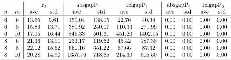
the MILP reformulation involving 108 possible combinations. We conducted experiments on (DQP) instances with convex and non-convex quadratic objective functions, respectively. The average values and standard deviations of the gaps are shown in Tables 3.1 and 3.2 with the following notations:
relgapP1 =
z1−z0
z0
, absgapP1 =|z1−z0|;
relgapP2 =
z2−z0
z0
, absgapP2 =|z2−z0|.
Table 3.1: (DQP) with convex quadratic objective function
z0 absgapP1 relgapP1 absgapP2 relgapP2
n m ave std ave std ave std ave std ave std
6 6 13.65 9.61 150.04 138.05 22.76 40.34 0.00 0.00 0.00 0.00 6 8 15.86 13.71 380.92 240.07 110.33 271.99 0.00 0.00 0.00 0.00 6 10 17.05 16.44 845.33 501.61 451.20 1402.15 0.00 0.00 0.00 0.00 8 6 21.36 13.01 233.17 119.62 45.42 187.38 0.00 0.00 0.00 0.00 8 8 22.12 15.62 661.16 351.22 57.66 87.32 0.00 0.00 0.00 0.00 8 10 20.28 14.90 1357.76 718.65 214.30 515.50 0.00 0.00 0.00 0.00
Table 3.2: (DQP) with non-convex quadratic objective function
z0 absgapP1 relgapP1 absgapP2 relgapP2
n m ave std ave std ave std ave std ave std
From Tables 3.1 and 3.2, we have some observations on the lower boundsz1andz2depending
on the convexity of objective function of (DQP):
1. The relative and absolute gaps with respect toz1 are large in both convex and non-convex
cases. Therefore, the relaxation (LCoR1) is not tight for general instances.
2. The gaps with respect to z2 are robust and close to zero in both convex and non-convex
cases. This indicates that the proposed RLT equality cuts are effective for tightening (LCoR1). Solving the proposed linear conic relaxation (LCoR2) can provide a high-quality
and robust lower bound for (DQP).
3. Regardless of whether the objective function of (DQP) is convex or not, as m or n in-creases, the relative gap between z1 and z0 becomes larger. It fits our general
under-standing that the tractable convex relaxations of the cone D∗(FP) are less accurate for
larger-size problems.
4. Both of the lower bounds z1 andz2 are more effective and robust for (DQP) with convex
rather than non-convex objective functions. Since the proposed approach is one kind of convex relaxation, it is reasonable that both of the relaxations (LCoR1) and (LCoR2)
may perform better in the convex case than the non-convex case.
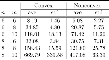
As to the computational efficiency of the proposed relaxation (LCoR2), we present the
computational timet2 of solving (LCoR2) in Table 3.3. We see that in either the convex case
or the non-convex case the computational efficiency of obtaining high-quality lower bounds by solving (LCoR2) is reasonable and stable.
Table 3.3: Computational timet2 (seconds) of solving (LCoR2)
Convex Nonconvex
n m ave std ave std
3.5
Extensions to constrained DQP problems
From Section 3.3, we know that the rank-two sufficient condition holds for (LCoR2) to guarantee
the zero gap. Numerical results in Section 3.4 further illustrate the effectiveness and robust-ness of the lower bounds provided by (LCoR2). Notice that problem (DQP) has no explicit
constraints except each variable being restricted to a finite set of discrete values. In this sub-section, we would like to extend the proposed linear conic relaxation framework to the discrete quadratic program with linear or quadratic constraints.
First, we consider the following linearly constrained discrete quadratic programming prob-lem:
min 1
2x
TAx+cTx
(DQPL) s.t. bTsx>Ls, s= 1, . . . , S, (3.18a)
xi∈ {di1, . . . , dim}, i= 1, . . . , n, (3.18b)
where A∈ Sn, c,b
s ∈ Rn and Ls ∈ Rfor s= 1, . . . , S. Following the approach introduced in Section 3.1, we can reformulate (DQPL) as
min 1
2u
TQu+qTu
(DQPL1) s.t. (3.5a),(3.5b),
gTsu>Ls, s= 1, . . . , S, (3.19)
where Q ∈ SN and q,g
s ∈RN, s = 1, . . . , S, i = 1, . . . , n. Based on the relaxation approach discussed in Section 3.2, we may generate additional RLT inequalities from the inequality constraints and choose the non-redundant ones as valid cuts. Then the proposed linear conic relaxation for (DQPL1) becomes
min 1
2Q•U +q
Tu
(DQPL2) s.t. (3.6a)−(3.6d),
gTsu>Ls, s= 1, . . . , S, (3.20a)
(gseTj)•U −LseTju>0, s= 1, . . . , S, j = 1, . . . , N, (3.20b)
−(gseTj)•U + (Lsej +gs)Tu>Ls, s= 1, . . . , S, j= 1, . . . , N.
extend the rank-two property to (DQPL2).
Theorem 3.5.1. If (DQPL2) has a rank-two optimal solution, then the gap between (DQPL2)
and (DQPL) is zero. In this case, the optimal solution of (DQPL) can be explicitly generated.
Proof. Assume that Y = 1 u
T
u U
!
is a rank-two optimal solution of (DQPL2). Since
rank(Y) = 2 andY satisfies (3.6a)-(3.6d), Theorem 3.3.4 explicitly generates ¯λ∈(0,1),u¯,v¯∈ RN such that
Y = ¯λ 1 ¯ u
!
1 ¯ u
!T
+ (1−¯λ) 1 ¯ v
!
1 ¯ v
!T
, (3.21)
and ¯u,v¯ satisfy (3.5a) and (3.5b). We now show that ¯u,v¯ satisfy constraints (3.19). Plugging u= ¯λu¯+ (1−λ)¯¯ v and U = ¯λu¯u¯T + (1−λ)¯¯ vv¯T into (3.20b)-(3.20c), we have
¯
λu¯j(gTsu¯−Ls) + (1−λ)¯¯ vj(gsTv¯−Ls)>0, (3.22)
¯
λ(1−u¯j)(gTsu¯−Ls) + (1−λ)(1¯ −v¯j)(gTsv¯−Ls)>0, (3.23)
forj= 1, . . . , N and s= 1, . . . , S. Because the 0-1 vectors ¯u,v¯ satisfy (3.2a) and ¯u6= ¯v, there exists an index j∗ ∈ {1, . . . , N} such that ¯uj∗ = 1 and ¯vj∗ = 0. Under j = j∗, (3.22) and
(3.23) are equivalent to (gTsu¯ −Ls) > 0 and (gsTv¯−Ls) > 0, respectively, for s = 1, . . . , S.
Therefore, we know that ¯u,v¯ are feasible solutions of (DQPL1). Notice that ¯u,v¯ and Y share
the same objective value in (DQPL1) and (DQPL2), respectively. Due to the optimality ofY,
its objective value is a lower bound for (DQPL1). Consequently, ¯u,v¯ are optimal solutions of
(DQPL1). In this case, the corresponding solutions of (DQPL) are optimal and there is no gap
between (DQPL2) and (DQPL).
Theorem 3.5.1 shows that the rank-two property holds for (DQPL2). However, when quadratic
constraints are added to (DQPL), the rank-two property may no longer hold for the
correspond-ing linear conic relaxation. Consider the followcorrespond-ing quadratically constrained discrete quadratic optimization problem:
min 1
2x
TAx+cTx
(DQPQ) s.t. (3.18a),(3.18b),
1 2x
TA
tx+cTtx>Rt, t= 1, . . . , T, (3.24)
min 1 2u
TQu+qTu
(DQPQ1) s.t. (3.5a),(3.5b),(3.19), 1
2u
TQ
tu+qtTu>Rt, t= 1, . . . , T, (3.25)
whereQ,Qt∈ SN and q,qt∈RN,t= 1, . . . , T;
min 1
2Q•U +q
Tu
(DQPQ2) s.t. (3.6a)−(3.6d),(3.20a)−(3.20c), 1
2Qt•U +q
T
t u>Rt, t= 1, . . . , T. (3.26)
Notice that the quadratic constraints (3.25) are relaxed to (3.26) in (DQPQ2), but there is no
related RLT constraint to tighten the relaxation. Following the proof of Theorem 3.5.1, given any rank-two feasible solution of (DQPQ2), we can generate ¯u,v¯ that satisfy the constraints
(3.6a)-(3.6d) and (3.20a)-(3.20c). Plugging the decomposition formula (3.21) into (3.26), we have
¯ λ(1
2u¯
TQ
tu¯+qtTu¯) + (1−λ)(¯
1 2v¯
TQ
tv¯+qtTv¯)>Rt, t= 1, . . . , T,
which do not lead to 12u¯TQtu¯+qtTu¯>Rt or 12v¯TQtv¯+qtTv¯>Rt. Consequently, we may not
generate feasible solutions of (DQPQ1) from the rank-two feasible solution of (DQPQ2).
Nevertheless, if we obtain a rank-two solutionY∗by solving the relaxation problem (DQPQ2)
via an SDP solver, the corresponding ¯uand ¯vwhich can be explicitly generated using the proof of Theorem 3.3.4 are still useful. The best situation is that both of ¯uand ¯vsatisfy the quadratic constraints (3.25), under which they become optimal solutions of (DQPQ1). If one of ¯uand ¯v is
feasible to (3.25), the feasible one may be close to an optimal solution of (DQPQ1). If none of ¯u
and ¯v satisfies the quadratic constraints, they can be used as starting solutions for additional processing.
3.6
Summary
solutions to the original DQP problem. We have also conducted numerical experiments on ran-domly generated DQP problems. The results indicate that the proposed linear conic relaxation can provide robust high-quality lower bounds for the original DQP problem. These bounds may be incorporated in a branch and bound scheme for providing optimal solutions to DQP problems in a more effective manner. The proposed linear conic relaxation approach and the rank-two property have been extended. We showed that the rank-two property holds for the corresponding linear conic relaxation of linearly constrained DQP problems.