DOI: 10.1051/epjconf/20111203001 C
Owned by the authors, published by EDP Sciences, 2011
Recent developments in analyses techniques
for non-destructive testing and assessment
of concrete properties
D. Breysse
aUniversité de Bordeaux, I2M, CNRS UMR5295, Civil and Environmental Engineering Department, 33405 Talence Cedex, France
Abstract. Non destructive techniques (NDT) offer many possibilities for evaluating concrete properties.
They can provide estimates of input data useful for assessing the residual service life or reliability of infrastructures, among them power plants. The issue is to know the quality of such estimates. The weaknesses of NDT have been pointed for a long time, since they are not considered as a reliable mean for providing quantitative data. Several recent research programs have resulted in significant improvements. Several issues are addressed here: (a) the adequacy of a NDT for a given purpose, (b) the quality/uncertainty of the material assessment provided by using one NDT, (c) the possibility of combining several techniques, so as to reduce the effect of uncontrolled parameters. For each of these issues, some general criteria are defined and it is explained how to derive quantitative information enabling their practical use in a decision process.
1. MAIN CHALLENGES FOR NON DESTRUCTIVE TESTING AND ASSESSMENT OF CONCRETE
The condition assessment of concrete is a key point when one wants to reassess existing structures whose material ageing can have resulted in some performance loss and some deterioration of the safety level. Progressive decay of performance also induces important maintenance costs, so as to prevent future deterioration and ultimate failure. Non-destructive techniques (NDT) are often used to assess the condition of existing reinforced concrete structures. The aims of NDT can be classified as being able to: (a) detect a defect or a variation of properties, between two structures or inside one structure, (b) build a hierarchy (i.e. to rank on a scale), regarding a given property, between several areas in a structure or between several structures, (c) quantify these properties, e.g. compare them to allowable thresholds. Detection, ranking and quantification can be regarded as three levels of requirements, the last being the strongest. Some authors have tried to synthesize the abilities of techniques with respect to given problems (Bungey et al. [1], Breysse and Abraham [2]) or to define the most promising paths for future developments (OECD [3], Naus [4]). Many case studies also exist where several techniques have been combined on a given structure (or on laboratory specimens), but a real added value is obtained only when the issue of combination has been correctly analyzed (Derobert et al. [5]). This added value can be defined in terms of: (a) accuracy of estimation, (b) relevance of physical explanations and diagnosis, (c) shorter time to reach a given answer. It remains to understand why and how combination can (or not) bring the expected added-value.
ae-mail:
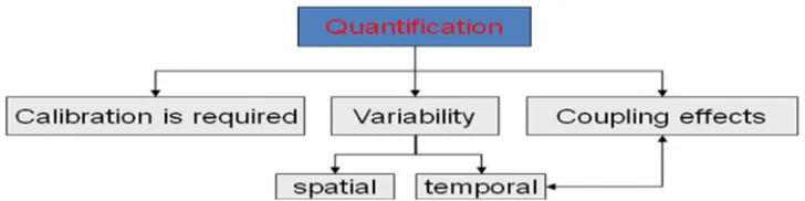
Figure 1. Main issues when wanting to use NDT to quantify concrete properties.
Among the main challenges for concrete assessment, one can cite: (a) stiffness and strength assessment since they are basic data for any structural evaluation, (b) water content (or moisture content) assessment, for two reasons: a large value of water content can be the sign of the bad quality of the material, but it can also be the sign that a potential vector of future damage is present, since the water is the more common agent for deterioration.
To summarize, when facing a problem of material assessment, the owner asks a series of questions: Q1. What technique(s) can / must be chosen?
Q2. How many tests are necessary?
Q3. Is it possible to derive a value for the property that is looked for? Q4. With what level of confidence?
A basic problem with engineering properties (like strength and modulus) is that they cannot be measured directly with NDT, which are only sensitive to physical and chemical properties. The main problems are summarized on figure1.
Thus one has to identify the relationships (either theoretical or empirical) between what is measured and what is expected for. Such relationships can thus be used on the basis on calibration curves/charts, and expected parameters can be derived. If X denotes the properties that are looked for and if Y denotes the result of the NDT measurement, using some Y=f(X) relationships (either theoretical or empirical) is necessary so as to deduce X values by solving this equation. But there is not any universal Y=f(X) relationship, and such an equation can only be used after a calibration step. It is the reason why European standards for on-site assessment of concrete strength EN 13791 [6] requires that the NDT measurements (obtained with rebound hammer, ultrasonic pulse velocity or pull-out tests) are calibrated, using a “basic curve” which fits the f(X) relationship to each specific case.
Safety and reliability assessment, which are key issues for usual structures but even more in nuclear engineering, also requires one is able to quantify the degree of spatial variability of material properties, since the structural response is mainly driven by the presence of weaker zones. NDT can provide an interesting way for assessing spatial variability, since they often allow a quick measurement of material properties, covering a wide surface and with no (or few) interaction with the material itself. In on-site conditions, time variability superimposes with spatial variability, and can prevent a simple analysis. It comes mainly from the influence of external parameters (e.g. temperature and humidity) which are not well controlled during the measurements (Klinghöfer et al. [7]). In such a situation, it is impossible to tell whether a difference between two values is either due to a real difference in material properties, or to a variation provoked by a change in the conditions of the measurement. This explains for instance most of the difficulties encountered when performing electrochemical measurements on concrete, which are very sensitive to environmental variations in humidity and temperature (Andrade et al. [8]). This question has been recently addressed by the author and will not be discussed here (Breysse et al. [9].
(ANR) (Balayssac [10], Lmdc [11]). The focus will be given on four X material properties: saturation ratio Sr, open (water) porosity p, Young’s modulus E and compressive strength fc. Other results have been obtained on the carbonation depth and chloride content, but they are not discussed here.
2. ON WHAT BASIS A TECHNIQUE CAN BE CHOSEN? WITH WHAT RESULT? 2.1 A research program devoted to assessment of NDT for concrete: focusing on variances The questions (Q1 to Q4) address the issue of choosing a relevant technique for a specific purpose (e.g. quantifying the water content, or the Young’s modulus of concrete). Once the technique is chose, one needs to know how many tests he must undertake and what will be the quality/accuracy of his assessment.
A recent research program, named SENSO, has been designed such as to quantify both the relations between material properties X (named “indicators”) and NDT results Y (named “observables”) and sources of uncertainties (measurement error Y, material variability at local and large scales, influence of uncontrolled factors) for a large series of NDT observables and concrete material properties (indicators), namely: strength, modulus, porosity, water content, carbonation depth, chloride content, magnitude of micro-cracking. The program was separated in several sub-programs, partly based on laboratory measurements and developments and partly on on-site measurements. The full program is not described here, where we only describe the methodology used for gathering useful data, evaluating the variability and building the empirical relationships between indicators and observables. On the basis of such relationships, a methodology for combining several NDT and evaluating the confidence of the assessment will be proposed in section3.
The first part of the program consisted in analyzing the effects of water content and porosity variations on the NDT observables for several concrete mixes, on laboratory specimens. Specimens are concrete slabs taken from 9 mixes in which are varied w/c (from 0.30 to 0.90), type, size and shape of aggregates. Eight slabs have been casted for each mix and all NDT measurements have been performed on all slabs. The first series of measurements is focused on porosity and water content influence, thus the saturation of slabs is controlled, and varied from a “saturated” reference condition to a “dry” condition. Many NDT techniques have been used by five research teams and consist in radar measurements, acoustical measurements, electrical measurements, infrared thermography measurements and capacimetry measurements. Each technique can provide a series of observables (f.i., for radar, velocity, magnitude or attenuation at several frequencies, shape of the signal...), leading to about 70 observables that have been defined and estimated on each specimen. Control tests have been performed on companion specimens, on cylinders and cores, and semi-destructive tests have been performed (Capo-test and rebound hammer).
Knowing the various sources of variability, the measurement process is defined such as to quantify, for each observable Y, several variance estimators:
- V1, coming from the lack of local repeatability of any measurement, at a given point, when the measurement is done several times. It is estimated after N repetitions (often 10 in laboratory measurements). This variance corresponds to the measurement errorY and averaging measurements provides a punctual value of the observable;
Table 1. Best selected NDT observables.
Family of NDT Measured quantity code unit
Y1 mechanical waves Velocity of surface waves US3c m.s−1 Y2 mechanical waves Velocity of compression waves US6 m.s−1
Y3 electrical Logarithm of Resistivity Re2 .m
Y4 radar (electromagnetic) Amplitude of the direct radar wave Ra1 without unit Y5 radar (electromagnetic) Time of flight of the radar wave Ra7c ns
- V3, coming from the “natural concrete” variability at global scale. It is evaluated by comparing the local representative value obtained at different points (in fact, average values obtained on 8 – normally identical - specimens are compared for laboratory measurements, and values obtained in different areas are compared during on-site measurements).
The variances are computed for each series of measurements and enable to derive, for each NDT:
Var (Y)=V1 (1)
Var (Yloc)=V2−V1 (2)
Var (Yglob)=V3−V2/N. (3)
2.2 What technique better fits a given purpose?
Analyzing variances enables to select the best observables, on the basis of the quality of fit of the regression and of the relative ratio between the sensitivity to indicator and the variability of the observable. The general idea is that a technique better fits a given purpose if: (a) it is sensitive to the indicator that is looked for, thus exhibiting a relatively high V3 value, (b) the measurement is accurate, thus exhibiting a relative large V3/V2 ratio. This ratio is a kind of signal to noise ratio, since it weights the influence of the variation one wants to detect (contrast) relatively to the variations due to non perfect repeatability. The lack of repeatability can be due either to material variability at very local scale, or to problems with the measurement device/process. It can also result from the influence of uncontrolled factors that will be discussed lower.
Two main results are thus available:
- the ranked list of useful observables for a given indicator,
- the relationships between indicators and observables, that can be used, after inversion, to identify the indicator value,
Five NDT observables will be considered in the following (Table 1). They are among the “best ones”, since they have a very good repeatability or/and they are sensitive to the indicators. They have been selected after a careful analysis of their quality/sensitivity (Breysse et al. [9]). These are:
- Two acoustical measurements: the velocity of surface waves and the velocity of compression waves,
- One electrical property: the resistivity,
- Two measurements provided by radar measurements: the amplitude of the direct wave signal and the time of flight of this wave.
Empirical multilinear relationships have been built for each observable and each pair of indicators (e.g. modulus and water content or modulus and saturation rate). The generic shape is:
Table 2. Sensitivity sX(Y) of five NDT measurements to four material properties (* denotes that, for this parameter, the analysis is done on the log(resistivity).
Y sSR sE sp sfc sE/sSR sSR/sE
Velocity of surface waves +12-13% +36% −36-37% +17% 2.8 0.4 Velocity of compression +11-12% +27% −29-30% +12% 2.3 0.4 waves
Resistivity* −35-36% +61% −66% +37% −1.7 −0.6
Amplitude of the direct −19% (+7-8%) (−13%) (+7-8%) −0.4 −2.3 radar wave
Time of flight of the radar +21% (−8-9%) (+9%) (−6%) −0.4 −2.4 wave
For instance, if indicators “saturation rate” and “saturated Young’s modulus” are considered:
Yi=Ai+BiSr+CiEsat (5)
For each Yiparameter and each X property, the Table2provides the sensitivity, defined as the ratio between the relative variation of Y and the relative variation of X:
sX(Y)=[Y/Y]/[X/X] (6)
A positive value of sX(Y) means that Y and X vary together, a negative value means that their variation is adverse. The larger the sensitivity, the more the technique is able to detect a variation of the X property. For instance, sX(Y)=12% means that if X experiences a 20% relative variation, Y will exhibit a 0.12 x 20=2.4% relative variation.
It can be seen that:
- Whatever X, the more sensitive technique is the resistivity, which confers it a convincing advantage,
- The two acoustical measurements are significantly sensitive to modulus and porosity, and, at a lesser degree, to saturation ratio,
- The two radar measurements are highly sensitive to saturation ratio. Regarding modulus, strength and porosity, the numbers are written in italics, since further investigation has shown that this sensitivity cannot be considered as statistically significant,
- The two last columns quantify the relative weights of the sensitivity to saturation ratio and modulus. The first three Y parameters are sensitive to both, but there is an important difference: for acoustic parameters, Sr and E influence Y in the same way (positive sensitivity) when resistivity is negatively influenced by saturation ratio and positively influenced by modulus. In other words, when E increases, all three Y values increase, but when Srincreases, acoustic velocities increase when resistivity decreases. Interesting consequences will be addressed in the following. Finally, radar techniques are mostly (if not exclusively) sensitive to Sr,
- Sensitivity values are also given for porosity p and strength fc. It appears that sp≈sE, which comes from the fact that modulus varies roughly linearly with porosity. Finally, the sensitivity to strength is roughly half that to modulus, which is consistent with the empirical relationship fc≈
√ E.
2.3 How many NDT tests are required?
Figure 2. Minimal number of measurements required to reach a given accuracy on Srvalue.
(V1 and V2). Thus one needs to repeat the measurements and to average the series of results, which enables to converge towards the “exact” solution.
From equation (5) and assuming that Sr is known, the value of the saturated modulus Esatcan be derived:
Esat=(Yi−Ai−BiSr)/Ci (7)
The quality of the estimate (assuming that the model is true) is related to the standard deviation sd(Yi) and to the number of measurements n which can be averaged such as to reach an average value. Assuming that the series of measurements follows a gaussian distribution of known standard deviation sd (Yi), one can say that, at the level of confidence (1−) the “true” average value E(Esat) belongs to the interval [+/−I] around the empirical average value, with I=k/2sd (Yi)/Ci
√ n.
Thus the minimal number N of measurements that are required so as to estimate the indicator at a given accuracy level+/−E(Esat) and at a given level of confidence can be derived:
n≥N=(k/2/C E(Esat))2.V3 (8)
The same can be done for any indicator. As a practical application, the Figure2plots the variation of N with regards to the expected range of accuracy of the estimate on Sr, for a 90% level of confidence. It can be read as follows: if one wants to estimate the Srvalue at+/−Sr, at least 2 measurements are needed for resistivity and time of flight, but 3 or 4 measurements for acoustic velocities and 9 measurements for the amplitude of radar wave. For the five NDT methods selected during the SENSO project, the required number of tests remains reasonable. The ranking between techniques is the same than that in Table2.
In practice, equation (8) can be used in different situations, including on-site measurements, as long as the model is assumed to remain the same. One has only to compute the new values of variance V3 corresponding to each case, which is straightforward from the Y measured values.
For instance, this rule has been applied to a series of on-site measurements (RC beams in the port of Saint-Nazaire, in oceanic environment, along the Loire river). Table3gives the minimum number of tests for obtaining Esatat+/−500 MPa. and a confidence level=90%.
Table 3. Minimum number of tests for the estimation of Esatat+/−500 MPa, and additional uncertainty for an uncertainty of+/−5 % on Srvalue.
observable Y1 Y2 Y3 Y4 Y5
number of tests 3 7 16 1796 44
additional uncertainty (MPa) +/−924 +/−1120 +/−1736 +/−5740 +/−5914
It must however be noted that these estimated numbers are probably optimistic, since they consider that the regression model is exact (that is certainly not true) and that the second indicator is known. If one considers that Srhas some uncertaintySr, the resulting uncertainty on Esatestimate is:
Esat= +/−BiSr/Ci (9)
The corresponding values are given on the last line of Table3. They correspond to the “coupling effect” of Figure1. The effect of the imperfect knowledge of Sr considered as a possible bias factor has non negligible consequences on the quality of identification of the indicator. The problem addressed here can be seen from a more general point of view, since it is that of any observable which is in fact sensitive to several indicators. It is the main reason explaining why one NDT measurement is often unable to provide directly the value of an indicator, even if it shows a high level of sensitivity and accuracy. This is the reason why it can really be interesting to try to combine several NDT measurements.
3. COMBINING NDT SO AS TO IMPROVE THE RELIABILITY OF CONCRETE ASSESSMENT
3.1 Establishing relevant criteria for an efficient combination of techniques
The principle underlying combination is to use two techniques, for solving problems in two cases: - when a first measurement is sensitive to two influential parameters, a second technique, sensitive
to one or two of these parameters, enables the inversion of the system (which has two equations and two unknowns) and the quantification of each parameter,
- if the first technique is sensitive to one influential parameter, but also to a bias factor (e.g., temperature) the bias effect can be reduced by measuring a second parameter which is also sensitive to this bias.
The “SonReb” method, which has been developed many years ago to estimate on site concrete strength (Malhotra [12]), is an example of such a combination. The Rebound number gives a first assessment of the concrete strength, which is corrected with Ultrasonic Pulse Velocity (UPV). In practice, the user can read the concrete strength in a chart where iso-strength curves are a combined function of Rebound and UPV. Even if this process has been widely criticized and is often used without care, the underlying principles deserve further attention. In fact, several conditions are required so as this method works:
- the two relationships (“models”) between the pair of indicators X1 and X2 and the pair of observables must be known, and the quality of fit must be as good as possible,
- this last condition is better checked if the ratio sensitivity/variance of the observable is larger, - the additional information is maximized when the two techniques show very different sensitivity
to the two parameters.
This can be illustrated in practice by using empirical relationships like those having the generic shape of equation (4) for Y1and Y2:
Y1=A1+B1X1+C1X2and Y2=A2+B2X1+B2X2 (10) One can express the “crossed sensitivity”:
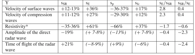
Figure 3. Bilinear model for the velocity
of compression waves.
Figure 4. Bilinear model for the resistivity.
whose absolute value must be as large as possible. G is minimal when B1C2=C2B1, i.e. when the two expressions are exactly proportional. In this case the second measurement only replicates the first one without carrying any new information. Each model can be represented by a plane in three dimensions, like in Figures3and 4 for two different techniques (ultrasonic velocity and electrical resistivity). The two measurements are complementary if the orientation of the two planes is clearly different.
Figures3and 4 show how the velocity of compression waves and the resistivity vary as a function of saturation ratio and Young’s modulus. The different orientations in space are compatible with the sensitivities of the Table1 and confirm that these two parameters do not bring the same information about the material properties. This different sensitivity is the key point when combining the techniques. The level at which their combination brings an added-value can be expressed:
- through the anglebetween the vectors perpendicular to the two planes: =arc cos[(1+B1B2+A1A2)/
√{
(1+B21+C21)(1+B22+C22)}] (12) - and (more exactly) through the angle ’ between two horizontal lines belonging to the two
respective planes:
=arc cos[(B
1B2+C1C2)/ √
{(B21+C21)(B22+C22)}] (13)
The larger the’ value, the better the theoretical added-value of the two techniques. The’ coefficient can be named “added-value index”. One can check that when G = 0, one has also=0. However, the theoretical added-value does not tell exactly what will be the efficiency of the combination, since it will be lowered for two reasons:
- the “measurement noise”, coming from errors including: (a) random errors and systematic errors, e.g. due to the processing device, (b) additional noise factors, among which low scale material variability (see equation (2)) and the influence of environmental factors (like temperature and humidity) not considered explicitly in the models.
1 1,2 1,4 1,6 1,8 2 2,2 2,4 2,6 2,8 3
0 0,2 0,4 0,6 0,8 1
Re 2 Ra 1
US 3c US 6
Ra 7c
Sr
(x100%)
p (x 10%)
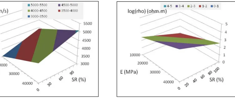
Figure 5. Regression lines enabling estimation of porosity and saturation rate from measurements of the various observables (see Table1for legend).
3.2 First practical application: Porosity and saturation assessment
A first example is given at Figure5that represents the projection onto the horizontal plane (porosity, saturation rate Sr) for a given series of measurements. The angles on this figure do not correspond to those calculated through equation (13) because of differences between the X-axis and Y-axis scales. The information provided by four out of the five observables is very consistent. The fifth one (radar measurement Y4-Ra1) gives a contradictory information. This comes from the model used for radar: a
multiregression linear model has been assumed a priori and the regression coefficients were identified and kept in the model. In fact, the Y4 dependency on porosity is statistically non significant and it
should have been removed from the model, keeping only the Sr dependency, thus resulting in vertical
line in Figure5. This lack of sensitivity of Y4to one indicator was yet discussed for number of tests in
Tables2and3: this observable provides a very reliable information on the saturation rate but it must be disregarded for porosity or Young’s modulus.
Figure 5 explains when the combination can works, since, as soon as two techniques show some significant added-value, the system inversion and the determination of the pair of indicators is possible. It also shows that the two US techniques (Y1-US3c, Y2-US6) provide consistent but redundant
information. If the assessment would be relying on these two methods only, the system of equations would be ill-conditioned and a large uncertainty would result.
3.3 Second practical example: Young’s modulus assessment
The second example describes the application of the same logic to Young’s modulus estimation, which is a common challenge for structural assessment. Sonic and ultrasonic measurements (UPV) are widely used for the condition assessment of building materials. For elastic materials, there is a theoretical relationship between the velocity of P-waves and the elasticity modulus E:
E=c V2Lor V2L =E/c (14)
where VLis the velocity of P-waves (in m.s−1),is the volumetric mass (in kg.m−3) and c is a constant
which depends on the Poisson ratioν. Thus, if linear elasticity is assumed and values are assigned toν and, the measurement of VLdirectly leads to a value of the Young modulus. Changes in environmental
conditions like relative air humidity modifies the water content in concrete, thus both Young modulus E and VL. Another difficulty is that the material mass densitymay change (as it is probably the case for
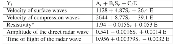
Table 4. Bilinear regression models for the five NDT parameters, where Sr and E are the saturation ratio (in %) and the Young’s modulus (in GPa).
Yi Ai+BiSr+CiE
Velocity of surface waves 1128+4.87Sr+26.4 E Velocity of compression waves 2644+8.77Sr+39.1 E
Resistivity* 1.94−0.015Sr+0.053 E
Amplitude of the direct radar wave 0.541−0.0016Sr+0.0014 E Time of flight of the radar wave 0.956+0.00379Sr−0.0032 E
fact that environmental conditions cannot be fully controlled influences: (a) the true indicator E, (b) the observable VL, (c) the relationship between E and VL.
Even if this relationship (model) has been calibrated (to better fit the specific context of a given concrete), any change in the environment induces model errors. Since UPV measurements are very easy to handle, they have been often combined to a secondary technique for material assessment. One approach is to combine them with another technique that is also sensitive to water content. Capacitive measurements (Sirieix et al. [13]), GPR measurements (Saisi et al. [14], Villain et al. [15]), IR thermography (Sirieix et al. [13], Kandemir-Yucel et al. [16]) or electrical resistivity (Sirieix et al. [13], Breysse et al. [17]) have been used for this purpose. However a more formal approach would be welcomed.
The Table4gives the equations corresponding to the models identified for material properties Srand E and the five NDT parameters (LMDC-SENSO [11]). The different signs of the partial derivatives (Bi and Cicoefficients) show that the added-value can be more or less important between these techniques.
The efficiency of combination is founded on several conditions:
- the two relationships (“models”) between the pair of properties X1 and X2 and the pair of measurements must be known, and the quality of fit must be as good as possible,
- this quality of fit is better if the sensitivity/measurement variability ratio (see Table2) is larger, - the two techniques must have a very different sensitivity to the two properties, i.e. very different
plane orientations on Figures3and 4.
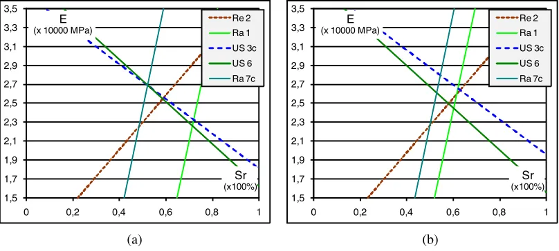
Figures6(a) and (b) show the regression lines corresponding to the measured values Yiin the Sr-E plane with the five observables Y1–Y5for two specimens (two slabs) made of the same concrete (w/c=0.55) and kept under the same conditions.
If both the measurements and the (statistical regression) models were perfect, all lines should cross in a unique point. If the material was homogeneous, the two graphs would be identical. Any difference between theory and practice is due to one of three causes: measurements are not perfect, the linear regression model is an approximation of the reality, and the material is not homogeneous. Thanks to their different slopes in this diagram, it is visible that techniques with mechanical waves (Y1/US3c and Y2/US6), the two radar measurements (Y4/Ra1 and Y5/Ra7c) and electric resistivity (Y3/Re2) really carry different information. The consistency between two techniques of the same family is also visible. The larger the difference between slopes, the better the added-value, with an optimum when the’ value provided by equation (13) is between 60 and 120◦. We can also note that the two radar measurements do not provide consistent results with the other techniques. This point has been discussed above.
1,5 1,7 1,9 2,1 2,3 2,5 2,7 2,9 3,1 3,3 3,5
0 0,2 0,4 0,6 0,8 1
Re 2 Ra 1 US 3c US 6 Ra 7c Sr (x100%) E
(x 10000 MPa)
1,5 1,7 1,9 2,1 2,3 2,5 2,7 2,9 3,1 3,3 3,5
0 0,2 0,4 0,6 0,8 1
Re 2 Ra 1 US 3c US 6 Ra 7c Sr (x100%) E
(x 10000 MPa)
(a) (b)
Figure 6. Use of linear regression model to identify the{Sr, E}values for two different concrete specimens (code
for techniques in Table1).
observables, the standard deviations sd are respectively:
sd (Y1)=41.2; sd (Y2)=11.5; sd (Y3)=0.11; sd (Y4)=0.025; sd (Y5)=0.020.
where sd stands for the square root of variance V3 from equation (3). These standard deviations correspond to coefficients of variation in the 1%–4% range. The smaller sd is, the more accurate the estimation of {Sr, E} will be after inversion. In addition, the knowledge of the standard deviation for
each measurement provides information about the level of accuracy of the estimate (a slightly different value of the measurement would correspond to a slight displacement of the line in the E-Sr diagram).
For instance, if one considers the resistivity measurement Y3, with sd(Y3)=0.11, this leads to an
uncertainty of about+/−0.11/0.015= +/−6% on Sr and of about+/−0.11/0.053= +/−2 GPa on E. Figure7provides the corresponding information. It is similar to Figures6a and b but only three techniques have been kept for the sake of clarity. For each technique, the bandwidth corresponding to +/−one standard deviation is drawn. It can be seen that US (US6–Y2) and resistivity (Re2–Y3) are
more efficient because of their smaller sd ranges than radar (Ra1–Y4).
Looking at the bandwidths also provides a range of values for {Sr, E} pairs directly visible in the
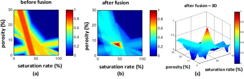
Figure7. It can be said that Young modulus ranges between 23 and 27 MPa and that saturation rate ranges between 50 and 65 %. However, since this range of estimate remains subjective, a more objective process has been developed, based on data fusion tools. The deterministic process of combination presented in the previous section has two main limitations:
- there is no information on the quality of the results and no confidence interval for estimated values, - there is no solution to the possible conflict between the solutions given by different observables. Data fusion offers an answer concerning these two weaknesses. It is based on the assumption that each measurement of an observable is linked with a distribution of probabilities of the indicators. The shape of the distribution (Yi) depends on the quality of the inversion (from observable to indicator), i.e.
from the quality of the measurement and from its sensitivity to the indicator. A specific data fusion software has been developed to be applied in the case of multiple measurements (Ploix et al [18]). Each measurement leads to a distribution of probability, for each {X1, X2} pair. All results provided bu the
1,5 1,7 1,9 2,1 2,3 2,5 2,7 2,9 3,1 3,3 3,5
0 0,2 0,4 0,6 0,8 1
Re 2 US 6 Ra 1
Sr (x 100 %) E
(x10000MPa)
Figure 7. Use of linear regression model to identify the {Sr, E} values with range of uncertainties (code for
techniques in Table1).
Figure 8. (a-c): Distribution of probabilities for porosity and saturation, originating from several ND methods (after
Ploix et al, [18]. Fig.8(a)–8(b): before and after fusion, Fig.8(c): 3D view.
X2. The central image shows what is obtained after the application of a mathematical operator for data
fusion. The last picture presents the same information in a 3D view.
Data fusion enables a visual representation that highlights the results and makes assessment easier. It uses an adaptive mathematical operator, for the assessment of the concordance between partial results provided by each observable (the concordance is maximum when there are no conflicts between the probability distributions originating from the different observables). It also provides the possibility to quantify a confidence index which is determined by analyzing the “solution peak” morphology.
4. CONCLUSIONS
Non Destructive Techniques are now developed at a degree such that they enable a quantitative assessment of concrete properties. This assessment requires that the more appropriate technique for a given purpose are selected, since each technique is more or less sensitive to each material property. This sensitivity is known for many NDTs and data available in the literature can be helpful. Table 2 provides information for saturation ratio, porosity, modulus and strength.
of other unknown parameters. The combination of two (or several) NDT measurements provides an effective answer, by uncoupling the effects of such parameters.
The final quality of the assessment depends on three items: (a) the measurement noise, mainly due to the quality of the technique, that can be quantified – this paper has explained how, while giving some representative values for several techniques, (b) the quality of the models used for inversion/identification, (c) the choice of the relevant techniques for each specific purpose, based on their (individual) sensitivities and how (when combined) they are complementary. Other advances have been recently made, for instance in the frame of the RILEM Technical Committee-INR 207, that has prepared recommendations on how to use techniques, separately or in combination, for a better assessment of concrete strength, of delamination or of unknown dimensions.
J.P. Balayssac, V. Garnier, J. Hugenschmidt, Z.M. Sbartai and, more generally all active members of ANR-SENSO program and of the RILEM-TC INR 207 are acknowledged for their contribution.
References
[1] Bungey J.H., Millard S.G., 1996, Testing of concrete in structures, 3rdedition, Blackie Acd and Prof., 286 p.
[2] Breysse D., Abraham O., Guide méthodologique de l’évaluation non destructive des ouvrages en béton armé, 2005, Presses ENPC, Paris.
[3] OECD Nuclear Energy Agency, 1998, Development priorities for Non-Destructive examination of concrete structures in nuclear plant, Nuclear Safety, NEA/CSNI/R(98), 25–39.
[4] Naus D.J., 2009, Inspection of nuclear power plant structures – overview of methods and related applications, Oak Ridge National Laboratory report, ORNL/TM-2007/191.
[5] Dérobert, X. , Garnier V., François D., Lataste J.F., Laurens S., 2005, Complémentarité des méthodes d’END, in Guide méthodologique de l’évaluation non destructive des ouvrages en béton armé, ed. Breysse D., Abraham O., Presses ENPC, Paris, 550 pages.
[6] EN 13791, Assessment of in-situ compressive strength in structures and precast concrete, CEN, Brussels, 28p., 2007.
[7] Klinghöfer O., Frolund T., Poulsen E., 2000, Rebar corrosion rate measurements fir service life estimates, ACI Fall Convention 2000, Committee 365 “Practical application of service life models”, Toronto, Canada.
[8] Andrade C., Alonso C. 1996 Corrosion rate monitoring in the laboratory and on-site, Constr. Build. Mater.; 10(5), 315-28.
[9] Breysse D., Klysz G., Dérobert X., Sirieix C., Lataste J.F., How to combine several non-destructive techniques for a better assessment of concrete structures, Cement and Concrete Research, Volume 38, Issue 6, June 2008, Pages 783-793.
[10] Balayssac J.P., 2008, SENSO: a French project for the evaluation of concrete structures by combining non destructive methods”, Sacomatis, RILEM conf., 1-2/9/2008, Varenna, It.
[11] LMDC-SENSO, Stratégie d’évaluation non destructive pour la surveillance des ouvrages en béton, final report, 274 p., 2009.
[12] Malhotra, V.M. (1981), Rebound, penetration resistance and pulse velocity tests for testing in place, The Aberdeen Group.
[13] Sirieix C., Lataste J.F., Breysse D., Naar S., Dérobert X., Comparison of nondestructive testing: infrared thermography, electrical resistivity and capacity methods for assessing a reinforced concrete structure, J. Building Appraisal 3, 1, 2007, 77-88.
[15] Villain G., Dérobert X., Abraham O., Coffec O., Durand O., Laguerre L., Baltazart V., 2009, Use of ultrasonic and elecromagnetic NDT to evaluate durability monitoring parameters of concrete, NDT-CE Conf., Nantes, France, 30 june – 3 jul. 2009.
[16] Kandemir-Yucel A., Tavukcuoglu A., Caner-Saltik E.N., 2007, Assessment of structural timber elements of a historic building by IR thermography and ultrasonic velocity, Infrared Physics and Tech., 49, 243-248.
[17] Breysse D., Yotte S., Salta M., Schoefs F., Ricardo J., Pereira E., Uncertainties in NDT condition assessment of corroding structures in marine environment, Medachs08 Conf., Lisbon, 28-30 jan. 2008.