Mitigating the One-Use Restriction in Attribute-Based Encryption

(1)

Mitigating the One-Use Restriction in Attribute-Based Encryption

Lucas Kowalczyk∗ Jiahui Liu† Tal Malkin‡ Kailash Meiyappan§

Abstract

We present a key-policy attribute-based encryption scheme that is adaptively secure under a static assumption and is not directly affected by an attribute “one-use restriction.” Our construction improves upon the only other such scheme (Takashima ’17) by mitigating its downside of a ciphertext size that is dependent on the maximum size of any supported attribute set.

1 Introduction

Attribute-based encryption (ABE) is a type of public key encryption which allows for fine-grained access control to encrypted data. In Key-Policy ABE, ciphertexts are associated with attributes, and secret-keys are associated with Boolean access policies that take in a set of attributes and return True if the key is capable of decrypting ciphertexts associated with that set and return False otherwise. Security guarantees that (potentially colluding) users without an authorized key should not be able to learn anything about an encrypted message. (A dual variant called Ciphertext-Policy ABE swaps the roles of attributes and access policies to be associated with the secret keys and ciphertexts respectively).

One way to make security proofs for ABE more attainable is to consider restricted notions of security. For KP-ABE, the notion of selective security requires the adversary to commit to a target set of attributes for the challenge ciphertext that will be attacked at the start of the security game. The earliest constructions of ABE using bilinear groups were proven secure in this model [GPSW06, Wat11].The notion of semi-adaptive security [JW14] requires the adversary to commit to a target set of attributes, but allows the adversary to see the public parameters first. These notions are obviously not realistic attack scenarios, so a KP-ABE scheme would ideally satisfy the notion ofadaptive security(full security), where the challenge attribute set can be chosen adaptively (in response to public parameters and any amount of secret keys received). The first construction of ABE achieving adaptive security appeared in [LOS+10], employing the dual system encryption methodology [Wat09] in its security reduction.

Another way to make proving security of ABE schemes easier is to reduce security to parameter-ized assumptions likeq-type assumptions, where the size of the elements included in the assumption’s challenge grows with some property of the adversary. q-type assumptions were used in the ABE constructions of [Wat11,LW12] to prove security. However, the security of dynamic assumptions like q-type assumptions is not well-understood, and the assumptions are often closely related to the scheme in which they are used. For example, the assumption may include a number of group

∗

Columbia [email protected]

†

‡

§

(2)

elements that scales with the number of queries made by the adversary in the security proof. Further, it is known that manyq-type assumptions become stronger as q grows [Che06], so we would ideally like to reduce security of ABE constructions to better understood assumptions of a static size, like the Decisional Linear Assumption (DLIN) or the Symmetric External Diffie-Hellman Assumption (SXDH).

A natural class of access policies one would like to be able to support in an ABE construction is that of general Boolean formulas. Unfortunately, it has proven tremendously difficult to construct efficient ABE for general Boolean formulas with adaptive security under static assumptions. All constructions except for [Tak17] suffer from a “one-use restriction.” That is, they only natively support read-once Boolean formulas, or formulas where attributes are used at most once in inputs. One way to extend such constructions to support formulas that use attributes more than once (say, k times) is to use k copies of new “meta-attributes” that stand for each use of the original attribute, and are handled as a group [LOS+10]. The downside of this approach is that it destroys the compactness of the construction – for KP-ABE, the size of the ciphertexts no longer depends on just the attribute set of the ciphertext, but also on the complexity of the formulas that the scheme supports (namely, the ciphertexts grow linearly with the maximum number of attribute uses in any formula supported). Ciphertexts associated with n0 attributes in a scheme like [LOS+10] where policies can reuse attributes at mostk times are of size O(n0·k).

Takashima presented the first KP-ABE scheme (proven adaptively secure from static assump-tions) with ciphertexts that do not grow directly with the number of attribute uses [Tak17], but unfortunately, the construction still has a dependence on the set of allowed policies. Specifically, ciphertexts are of sizeO(n+r), where nis the maximum size of any supported attribute set andr

is the maximum number of columns in any policy matrix supported (this is the policy dependency). For (fan-in 2) Boolean formulas, standard techniques [LW11a] to translate the formula into a policy matrix result in r being equal to the number of AND gates in the formula. Additionally, this dependence onn, the maximum size of any supported attribute set rather than only the attribute set of the relevant ciphetext is undesirable, since one can imagine the size of each ciphertext’s associated attribute set varying wildly from the worst-case maximum-sized set supported by the system. In fact, it is unclear whether O(n+r)-size ciphertexts are ever an asymptotic improvement over the O(n0·k)-size ciphertexts of all other known ABE schemes proved adaptively secure under static assumptions.

1.1 Our Result

In this work, we describe a KP-ABE construction that mitigates one of the two undesirable dependencies of [Tak17], featuring ciphertexts of sizeO(n0+r) instead ofO(n+r) (while remaining adaptively secure from a static assumption: the Symmetric Diffie-Hellman Assumption (SXDH) and allowing the reuse of attributes in its monotone span program policies). This significant improvement allows us to rigorously argue that there exist classes of access policies for which our construction enjoys an asymptotic improvement over the state of the art. We note that our construction is for the small-universe setting, where attributes come from a polynomial (in the security parameter) sized universe that is fixed upon setup, whereas the construction of [Tak17] supports an attribute universe that may be exponentially large. This allows us to focus on the techniques required to asymptotically improve the ciphertext size. Our scheme is likely translatable to accommodate a large attribute universe without sacrificing asymptotic efficiency, but we leave this for future work.

(3)

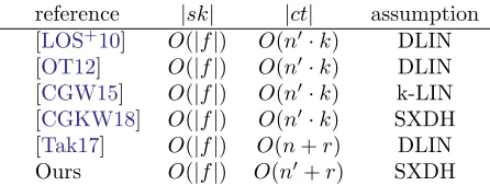
reference |sk| |ct| assumption [LOS+10] O(|f|) O(n0·k) DLIN [OT12] O(|f|) O(n0·k) DLIN [CGW15] O(|f|) O(n0·k) k-LIN [CGKW18] O(|f|) O(n0·k) SXDH [Tak17] O(|f|) O(n+r) DLIN Ours O(|f|) O(n0+r) SXDH

Figure 1: Summary of several KP-ABE schemes proven adaptively secure under static assumptions for monotone span programs. Here, n0 is the number of attributes associated to the ciphertext,n

is the maximum size of any supported attribute set,r is the maximum number of columns in any policy matrix, andk is the maximum number of attribute reuses in any policy (except in the name for the “k-LIN” assumption, which is unrelated and an unfortunate overloading).

assumption as an interesting open problem.

1.2 Comparing Perfomance

Figure 1contains a comparison of several KP-ABE schemes proven adaptively secure under static assumptions for monotone span programs.

An obvious question in comparing our construction to the state-of-the-art is: how doesrcompare to k? Is n0+r ever better thann0·k? It is easy to come up with individual formulas where this is the case, but it’s not obvious that such a formula can’t always be “compressed” to an equivalent formula that has less attribute-reuse. In general, circuit/formula minimization questions like this are difficult to answer.

Fortunately, we can make a simple counting argument to show that indeed there are classes of functions which cannot be expressed using Boolean formulas with much smaller maximum attribute reuse than the maximum number of AND gates within the class. To see this, consider some subset of xattributes in the attribute universe. There are 22x Boolean functions on these attributes, and we can express each function as a DNF in the naive way as a formula that uses at most O(2x) AND gates. So, for this class of functions, r=O(2x).

However, counting the number of different Boolean formulas that could attempt to realize these functions using a maximum kreuses of any attribute shows that at leastk= Ω(2x) attribute-reuses are required to realize all of the functions in this class. In this case, we see our construction enjoys a multiplicative to additive improvement (from n0·Ω(2x) to n0+O(2x)).

1.3 Technical Details

Our construction can be seen as combining the best of both worlds between the construction of [Tak17], which is the first to not directly depend on the number of attribute-reuses (while adaptively secure from a static assumption), and the lineage of [GPSW06,LOS+10,KL15,CGKW18], which enjoys ciphertexts that are independent of the size of the attribute universe (they depend only on the number of attributes actually associated with the ciphertext).

Specifically, all of these schemes are based on linear secret sharing and are built using bilinear groups. Given a matrix M representing a monotone span program, linear secret shares of α are constructed by choosing randomness ri, then computing M ·(α, r2, ..., rm) to obtain a vector of

shares~λ. [GPSW06, LOS+₁₀_, _KL15_, _CGKW18_{] embed these shares into their constructions’ secret}

(4)

{gλj+aρ(j)yj_, _gyj_}

j∈M

Figure 2: Example secret key

[Wat09] of adaptive security occurs when secret shares in the dual “semi-functional” space of a secret key are changed from sharing 0 to sharing a random elementα0 (in [LW12], this is the change from “nominal semi-functional” to “temporary semi-functional”). This is the step of the proof that uses the fact that the keys requested by an adversary are not allowed to decrypt the challenge ciphertext, to argue that there exists different randomness r_i0 where a sharing of 0 using the ri

randomness looks identically distributed to a sharing of random α0 using the r_i0 randomness, as long as the only shares seen are not allowed to reconstruct the secret. Crucially, the alternative randomnessr0_i is not defined until the challenge ciphertext is requested (as the challenge ciphertext defines which shares in the key are allowed to be seen). The constructions in the [LOS+10] lineage therefore require that the change in the secret shares in their keys be information theoretic (so they can be implicitly changed upon challenge ciphertext creation). This turns out to be the root of the one-time attribute use restriction (reusing attributes prevents this information-theoretic argument from working).

[Tak17] employs a technique of delayed share construction to get around this problem. Specifically, the construction does not construct a secret sharing {λj} which is embedded in the secret key,

but instead keeps the components that generate λj (vectors M~j and (α, r2, ..., rm)) separateuntil

decryption. The M~j portion is embedded in the key and the randomness (α, r2, ..., rm) is stored

in the ciphertext. Decryption computes the dot product of these two components to implicitly construct λj that function in the same way as before. The advantage of this approach is that the

randomness used in the secret shares is not needed until the challenge ciphertext is requested, so computational assumptions can be used to side-step the one-time attribute use restriction that comes with information-theoretic changes.

Like [LOS+10], [Tak17] also masks secret key components, making them only available to ciphertexts associated with the appropriate attributes. However [Tak17] does this via a somewhat blunt tool: namely, its secret keys contain a vector~y which can encode orthogonality relationships with any subset of the attributes associated with a ciphertext and whose length is as large as the maximum attribute set supported by the system.

In contrast, the “share encapsulation” in [LOS+10] demonstrated in Figure2 can be thought of as using a vector of dimension 2 to perform the same job. (aρ(j)yj, yj) is being used to hide the share

λj and share retrieval will be allowed only give a ciphertext with an “orthogonal” vector: (s,−saρ(j)). Our construction can be seen as essentially replacing [Tak17]’s vector~y with constant-dimensioned vectors like this, resulting in a ciphertext dependent only on the number of attributes associated with it, just like all previous schemes. Essentially, an information-theoretic “encapsulation” argument supported by the vector~y for all shares is replaced with a computational one using a vectors of a constant size for each attribute. Doing so makes the dual-system hybrid more delicate, as it requires careful management of rerandomization across the now greatly reduced dimensions. More detail about how the proof structure handles this is provided in Section5.2.

1.4 Related Work

Additional work on ABE in the bilinear setting includes various constructions of KP-ABE and CP-ABE schemes (e.g. [BSW07,OSW07,GJPS08,JW14]), schemes supporting multiple authorities (e.g. [Cha07,CC09,OT13,LW11a]), and schemes supporting large attribute universes

(5)

The construction of [GVW13] supports circuit access policies rather than monotone span programs or Boolean formulas, which makes it more expressive than any known bilinear scheme. It was proven selectively secure under the standard LWE assumption. The construction of [BV16] later extended this to semi-adaptive security for circuit access policies from LWE. Proving full adaptive security for a ABE scheme supporting circuits from LWE or an assumption on bilinear maps is an interesting open problem.

Circuit policies are supported by the construction in [GGH+13] based on multilinear maps. This scheme is proven selectively secure, under a particular computational hardness assumption for multilinear groups. The multilinear scheme in [GGHZ14] achieves adaptive security, relying on computational hardness assumptions in multilinear groups.

2 Preliminaries

We will writea←_Z_p to denote choosingauniformly at random from setZp and will abuse notation

to usej∈M as a subscript to denote each index j of the rowsMj of matrix M.

2.1 Prime Order Bilinear Groups

We construct our system in prime order asymmetric bilinear groups. We let G denote a group

generator - an algorithm which takes a security parameterλas input and outputs (p, G, H, GT, e),

where p is a prime,G, H andGT are cyclic groups of orderp, ande:G×H→GT is a map with

the following properties:

1. (Bilinear)∀g∈G, h∈H, a, b∈_Zp, e(ga, hb) =e(g, h)ab

2. (Non-degenerate) ∃g∈G, h∈H such thate(g, h) has order p inGT.

We refer to G, H as thesource groups and GT as thetarget group. We assume that the group

operations in G, H and GT and the mapeare computable in polynomial time with respect to λ,

and the group descriptions ofG, H and GT include a generator of each group.

2.2 Dual Pairing Vector Spaces

We will employ the concept of dual pairing vector spaces from [OT08,OT09], where we’ll denote choosing random dual orthogonal bases as: (B,B∗) ← Dual(Znp). Such bases are collections of

linearly independent vectors chosen at random up to orthogonality constraints (~bi·~b∗_i = 1,~bi·~b∗_j = 0

for i 6= j). For example, one can implement Dual(Znp by choosing a random invertible matrix

B, setting B :=B which then defines B∗ as B∗ := (B−1)T. Note that the dual basis generation

procedure satisfies the property that, ifRis an invertible matrix, then (B,B∗) and (R·B,(R−1)T·B∗)

are distributed identically when (B,B∗)←Dual(Znp). We will use this fact in our security proof to

introduce new randomness into free dimensions of the construction as well as to embed computational assumptions. Finally, we will writeg~v to denote the vector of group elements (gv1_{, ..., g}vn_{), and will}

use the notation: (x1, ..., xn)B to denotegx1~b1·...·gxn~bn.

2.3 Complexity Assumptions

The security of our system will be reduced to the Symmetric External Diffie-Hellman assumption (SXDH). We use the notationx←S to express that elementx is chosen uniformly at random from

(6)

Symmetric External Diffie-Hellman Assumption (SXDH) The SXDH problem in G is stated as follows: given an asymmetric bilinear group (G, H) of prime order p with respective generatorsg, h, and givenga, gb and T =gab+r∗∈Gwhere a, b←Zp and either r∗= 0 orr ←Zp,

output “yes” ifr is a random element ofZp and “no” otherwise. The SXDH problem inH is stated

symmetrically, swapping the role of Gand H.

Definition 1. SXDH Assumption in (G, H): no polynomial time algorithm can achieve non-negligible advantage in deciding the SXDH problem in Gor the SXDH problem in H.

2.4 Background for ABE

We now give required background material on Linear Secret Sharing Schemes, the formal definition of a KP-ABE scheme, and the security definition we will use.

2.4.1 Monotone Span Programs / Linear Secret Sharing Schemes

Our construction uses linear secret-sharing schemes (LSSS) to realize monotone span program access structures [MW93]. We use the following definition (adapted from [Bei96]). In the context of ABE, attributes will play the role of parties and will be represented as indexesi∈[|U |] for a fixed universe

U.

Definition 2. (Linear Secret-Sharing Schemes (LSSS)) A secret sharing scheme Π over a set of attributes is called linear (over Zp) if

1. The shares belonging to all attributes form a vector over Zp.

2. There exists an `×n matrix Λ called the share-generating matrix for Π. The matrix Λ has ` rows andn columns. For all j= 1, . . . , `, the jth row of Λis labeled by an attributei=ρ(j)

(ρ is a mapping that maintains the relationship between matrix rows and attributes). When we consider the column vector v= (s, r2, . . . , rn), where s∈Zp is the secret to be shared and

r2, . . . , rn∈Zp are randomly chosen, thenΛvis the vector of `shares of the secret saccording

toΠ. The share(Λv)j =λj belongs to attribute i=ρ(j).

We note the linear reconstruction property: we suppose that Π is an LSSS. We letS denote an authorized set. Then there is a subset S∗ ⊆S such that the vector (1,0, . . . ,0) is in the span of rows of Λ indexed by S∗, and there exist constants {ωi ∈Zp}i∈S∗ such that, for any valid shares

{λi} of a secret s according to Π, we have:

X

i∈S∗

ωiλi = s. These constants {ωi} can be found in

time polynomial in the size of the share-generating matrix Λ [Bei96]. For unauthorized sets, no such

S∗,{ωi}exist.

For any set S of unauthorized shares, since the vector (1,0, ...,0) is not in the span of rows indexed by S, then there is some vectorw~ that is orthogonal to all of the rows of Λ indexed by S

but is not orthogonal to (1,0, ...,0). By scaling this vector, we can maintain these orthogonality relationships and force the first coordinate w1 to be 1. Our proof of security will use the existence of this vector.

2.4.2 KP-ABE Definition

(7)

Setup(λ,U)→(PP,MSK) The setup algorithm takes in the security parameterλand the attribute universe description U. It outputs the public parameters PP and a master secret key MSK.

Encrypt(PP, m, S) → CT The encryption algorithm takes in the public parameters PP, the messagem, and a set of attributesS. It will output a ciphertext CT. We assume thatS is implicitly included in CT.

KeyGen(MSK,PP,A)→SK The key generation algorithm takes in the master secret key MSK,

the public parameters PP, and an access structureA over the universe of attributes. It outputs a

private key SK which can be used to decrypt ciphertexts encrypted under a set of attributes which satisfiesA. We assume thatAis implicitly included in SK.

Decrypt(PP,CT,SK) → m The decryption algorithm takes in the public parameters PP, a ciphertext CT encrypted under a set of attributesS, and a private key SK for an access structure A.

If the set of attributes of the ciphertext satisfies the access structure of the private key, it outputs the messagem.

2.4.3 Adaptive Security for KP-ABE Systems

We define adaptive security for KP-ABE Systems in terms of the following game:

Setup The challenger runs the Setup algorithm and gives the public parameters to the attacker.

Phase 1 The attacker queries the challenger for private keys corresponding to access structures.

Challenge The attacker declares two equal length messagesM0, M1 and a set of attributesA⊆ U where U is the attribute universe such that A does not satisfy the access structure of any of the keys requested in Phase 1. The challenger flips a random coin β∈ {0,1}, encryptsMβ underS to

yield ciphertext CTβ and gives CTβ to the attacker.

Phase 2 The attacker queries the challenger for private keys corresponding to access structures that are not satisfied byS.

Guess The attacker outputs a guess β0.

Definition 3. The advantage of an attackerA in this game is defined asAdv_AKP−ABE(λ) = Pr[β =

β0]− 1 2.

Definition 4. A key-policy attribute based encryption scheme is adaptively secure if no polynomial time algorithm can achieve a non-negligible advantage in the above security game.

3 Construction

Setup(λ,U) → P P, M SK The setup algorithm chooses an asymmetric bilinear group G(λ) →

(8)

chooses valuesai←Zp. It then generates random dual orthonormal sets:

(D,D∗)←Dual(Z6p)

(B,B∗)←Dual(Z3(pr+1))

(Ai,A∗i)←Dual(Z3p) for i∈[k]

The public parameters P P are:

e(g, h)

(~e1)D∗,(~e2)D∗ {(~ei)B∗}i∈[r+1] {(ai,0,0)A∗i}i∈[k]

The MSK is:

(~e1)D,(~e2)D {(~ei)B}i∈r+1 {(1,0,0)_Ai}i∈[k]

Such a construction is equipped to create keys for access policies which include attributes i∈ U.

Encrypt(m, S, P P) → CT The encryption algorithm draws α,∆, s, zi ← Zp (for i ∈ [r]) and

forms the ciphertext as:

CTS= (C0, C1, C2,{C3,i}i∈S)

where

C0 :=m·e(g, h)α

C1 := (α,−∆, ~02, ~02)D∗

C2 := (∆, z2, ..., zr, s, ~0r+1, ~0r+1)B∗

C3,i := (sai,0,0)A∗i

(This implicitly includes S)

KeyGen(M SK, M, P P) → SK The key generation algorithm takes in the public parameters, master secret key, and LSSS access matrixM. It chooses a random exponentx←Zp. For each row

j (associated with attributeρ(j)) in the policy matrixM, it chooses exponent yj ←Zp and outputs

the secret key:

SKM = (K1,{K2,j, K3,j}j∈M)

where:

K1 := (1, x, ~02, ~02)D

K2,j := (——x ~Mj——, aρ(j)yj, ~0r+1, ~0r+1)B

(9)

Decrypt(CTS, SKM, P P) → m Given ciphertext CTS = (C0, C1, C2,{C3,i}i∈S) and secret key

SKM = (K1,{K2,j, K3,j}j∈M), ifSsatisfiesM, then there is a setS∗ of policy row indices such that

j∈S∗ =⇒ ρ(j)∈Sand there exist efficiently computable constantsωj such that

X

j∈S∗

ωjMj·~z= ∆

(recall section 2.4.1). The decryption algorithm computes these ωj and then computes:

B = Y

j∈S∗

e(C2, K2,j)ωj·e(C3,ρ(j), K3,j)ωj

D=e(C1, K1)

and finally, computes and outputs:

C0

B·D =m

4 Correctness

This scheme satisfies correctness since:

B = Y

j∈S∗

e(C2, K2,j)ωj·e(C3,ρ(j), K3,j)ωj

= Y

j∈S∗

e (∆, z2, ..., zr, s, ~0

r+1_{, ~}₀r+1₎

B∗, (——x ~Mj——, aρ(j)yj, ~0r+1, ~0r+1)B

!ωj

·e ( saρ(j),0,0)A ∗ ρ(j), (−yj,0,0)Aρ(j)

!ωj

= Y

j∈S∗

e(g, h)xωjλj+sωjaρ(j)yj _·_e₍_{g, h}₎−sωjaρ(j)yj

=e(g, h)

xX j∈S∗

ωjλj

=e(g, h)x∆

D=e(C1, K1)

=e (α,−∆, ~0

2_{, ~}₀2₎

D∗ (1, x, ~02_{, ~}₀2₎

D

!

=e(g, h)α−x∆

and finally:

C0

B·D =

m·e(g, h)α

e(g, h)x∆_·_e₍_{g, h}₎α−x∆

=m

5 Proof of Security

(10)

5.1 Auxiliary Ciphertext and Secret Key Distributions

The security proof is a dual system hybrid over a sequence of games with different types of keys and ciphertexts. In these definitions, w~ is the vector described in Section2.4.1, which is defined relative to the policy of the ith requested secret key in hybrid games superscripted byi (and is orthogonal to the rows of M in theith key which are associated with attributes in the challenge ciphertext, while having a first coordinate of 1).

Note that we omit the message encapsulation component m·e(g, h)α from each semi-functional ciphertext description, since it is the same for all variants. Unless specifically mentioned, the distributions of all elements remain‘ unchanged from the last time they were defined.

Type0 Type 0 keys and ciphertexts are simply the keys and ciphertexts of the regular construction.

CT0:=

  α −∆ 0 0 0 0   D∗  

∆ z2 . . . zr s

0 . . . 0 0 . . . 0

  B∗        −sai

0 0





A∗i



 

 

i∈S

SK0 :=

  1 x 0 0 0 0   D       

xM1,j xM2,j ... xMr,j aρ(j)yj

0 0 ... ... 0

  B   yj 0 0  

Aρ(j)



 

 

j∈M

Type1

CT1 :=





α −∆ 0 −∆0 0 −∆0





D∗





∆ z2 . . . zr s

∆0w~ s0

∆0w~ s00

  B∗        −sai

−s0ai

−s00ai





A∗i



 

 

i∈S

wheres0, s00∆0 ←Zp (andw~ is defined relative to the policy of theith requested secret key in hybrids

superscripted byi).

SK1:=SK0

Type2

CT2:=CT1

SK2:=





1 x

0 x0

0 0   D       

x0M1,j x0M2,j ... x0Mr,j 0

0 0 ... ... 0

  B   yj 0 0  

Aρ(j)



 

 

j∈M

where x0 ←_Z_p.

Type3,k Keys of Type 3 to Type 11 are also subindexed byk, which runs from 1 to r: which is

the number of rows in the key’s policy matrix. In all types, theK1 component of the secret key remains the same as in Type 3. The (K2,j, K3,j) components for j < k are the same as inSK11,k−1. These components for j > k (up to r) are the same as in SK2. The kth (K2,k, K3,k) components of

the key of Type3,k are described below:

(11)

SK3,k :=





xM1,k xM2,k ... xMr,k aρ(k)yk

x0M1,k+t1 x0M2,k+t2 ... x0Mr,k+tr 0

−t1 −t2 ... −tr 0

  B   yk 0 0  

Aρ(k)

Type4,k

CT4,k :=CT2

SK4,k :=





0 0 ... 0 0

x0M1,k x0M2,k ... x0Mr,k 0

  B   yk 0 0  

Aρ(k)

Type5,k

CT5,k :=CT2

SK5,k :=





0 0 ... 0 0

x0M1,k x0M2,k ... x0Mr,k aρ(k)y0k

  B   yk 0

y0_k





Aρ(k)

Type6,k

CT6,k :=





α −∆ 0 −∆0 0 −∆0





D∗





∆ z2 . . . zr s

∆0w~ s0

∆0w~ s00

  B∗        −sai

−s0ai

−s00ai





A∗i



 

 

i6=ρ(k)∈S

[        −sai

−s0ai

−s00˜ai





A∗i



 

 

i=ρ(k)∈S

Note that the only difference fromCT2 is in the vector for attributei=ρ(k), if it is in the setS.

SK6,k :=





0 0 ... ... 0

x0M1,k x0M2,k ... x0Mr,k ˜aρ(k)y0k

  B   yk 0

y0_k





Aρ(k)

(recall that the (K2,j, K3,j) components forj6=kare the same as in Type5,k)

Type7,k

CT7,k:=CT6,k

SK7,k :=





0 0 ... ... 0

x∗M1,k x∗M2,k ... x∗Mr,k a˜ρ(k)yk0

  B   yk 0

y_k0





Aρ(k)

(12)

Type8,k

CT8,k :=CT2

SK8,k :=





0 0 ... ... 0

x∗M1,k x∗M2,k ... x∗Mr,k aρ(k)yk0

  B   yk 0

y_k0





Aρ(k)

Type9,k

CT9,k :=CT2

SK9,k :=





0 0 ... ... 0

x∗M1,k x∗M2,k ... x∗Mr,k 0

  B   yk 0 0  

Aρ(k)

Type10,k

CT10,k :=CT2

SK10,k:=





−t1 −t2 ... −tr 0

x∗M1,k+t1 x∗M2,k+t2 ... x∗Mr,k+tr 0

  B   yk 0 0  

Aρ(k)

Type11,k

CT11,k :=CT2

SK11,k :=





x∗M1,k x∗M2,k ... x∗Mr,k 0

0 0 ... ... 0

  B   yk 0 0  

Aρ(k)

Type12

CT12:=CT2

SK12:=





1 x

0 x0

0 0   D       

0 0 ... 0 0

0 0 ... ... 0

  B   yj 0 0  

Aρ(j)



 

 

j∈M

Type13

CT13:=





α −∆ 0 −∆0 0 −∆0





D∗





∆ z2 . . . zr s

∆0~e1 s0 ∆0~e1 s00

  B∗        −sai

−s0ai

−s00ai





A∗i



 

 

i∈S

(13)

Type14

CT14:=CT13

SK14:=





1 x

0 x0

0 0   D       

x0λj 0 ... ... 0

0 0 ... 0 0

  B   yj 0 0  

Aρ(j)



 

 

j∈M

where λj :=M~j·(1, z20, ..., zr0) forzi0 ←Zp.

Type15k Type 15 keys and ciphertexts are subindexed byk which runs from attribute 1 to|U |.

CT15k :=CT14

SK15k :=





1 x

0 x0

0 0   D       

x0λj 0 ... ... a˜ρ(j)yj0

0 0 ... 0 0

  B   yj

y0_j

0





Aρ(j)



 

 

j∈Mwhereρ(j)≤k, ρ(j)6∈S

[       

x0λj 0 ... ... 0

0 0 ... 0 0

  B   yj 0 0  

Aρ(j)



 

 

j∈M whereρ(j)> korρ(j)∈S

Type₁₅_/₁₆

H Type 15/16H keys are a halfway point between Type 15|U | and Type 16|U | keys, where

the ˜a_ρ₍_j₎yj are changed into freshly random ˜aj0 for each j where ρ(j) 6∈ S by embedding SXDH

challenge.

CT15H =CT16H :=CT14

SK15H :=





1 x

0 x0

0 0   D       

x0λj 0 ... ... ˜a0jyj0

0 0 ... 0 0

  B   yj

y_j0

0





Aρ(j)



 

 

j∈M whereρ(j)6∈S

[       

x0λj 0 ... ... 0

0 0 ... 0 0

  B   yj 0 0  

Aρ(j)



 

 

j∈M whereρ(j)∈S

SK16H :=





1 x

0 x0

0 0   D       

x∗λj 0 ... ... ˜a0jyj0

0 0 ... 0 0

  B   yj

y_j0

0





Aρ(j)



 

 

j∈M whereρ(j)6∈S

[       

x∗λ0_j 0 ... ... 0

0 0 ... 0 0

  B   yj 0 0  

Aρ(j)



 

 

j∈M whereρ(j)∈S

(14)

Type16k Type 16 keys and ciphertexts are also subindexed byk which runs from attribute 1 to

|U |.

CT16k :=CT15k

SK16k :=





1 x

0 x0

0 0   D       

x∗λ0_j 0 ... ... a˜_ρ₍_j₎y0_j

0 0 ... 0 0

  B   yj

y0_j

0





Aρ(j)



 

 

j∈Mwhereρ(j)≤k,ρ(j)6∈S

[       

x∗λj 0 ... ... 0

0 0 ... 0 0

  B   yj 0 0  

Aρ(j)



 

 

j∈M whereρ(j)> korρ(j)∈S

Type17

CT17:=CT161

SK17:=





1 x

0 x0

0 0   D       

0 0 ... ... 0

0 0 ... 0 0

  B   yj 0 0  

Aρ(j)



 

 

j∈M

Type18

CT18:=





α∗ −∆

0 −∆0





D∗





∆ z2 . . . zr s

∆0~e1 s0 ∆0~e1 s00

  B∗        −sai

−s0ai

−s00ai





A∗i



 

 

i∈S

where α∗ ←_Zp.

SK18:=SK17

5.2 Hybrid Structure

Our proof of security will consist of a hybrid sequence of games where the keys and challenge ciphertext are constructed according to various types. At a high level, the proof follows a typical dual-system hybrid structure, where the challenge ciphertext is first made “semi-functional,” then the hybrid continues over the secret keys requested, transforming each key into a “semifunctional” variant which is useless to the attacker relative to the challenge (semifunctional) ciphertext.

(15)

captioned “SF-Key Before” in Figure 3). This bifurcated approach to handling secret keys in a dual-system proof was first employed in [LW12] and later refined by [Att14,Att16]

A key step in our proof (and of [Tak17]) is Lemma13, where each policy matrix row is isolated in turn against the ciphertext’s w~ alternative randomness component and their dot product’s distribution is used to argue that the row can be multiplied by an uncorrelatedx∗. In [Tak17], this argument takes advantage of the inefficient~y vector, but for us, we need to delicately thread just enough randomness through the single attribute element ai hiding each row to accomplish the same

feat. We accomplish this in Lemma 12.

Our hybrid starts with Gamereal, the real security game. This has all keys and cipher texts

of type Type0. We then proceed through a sequence of games Gameij, which are indexed by each

requested keyiand subhybrid index`. LetQ1 be the number of key queries issued by the adversary before the challenge ciphertext, and let Q2 be the number of key queries issued by the adversary after the challenge ciphertext.

Definition 5. In Game`_i for i≤12, the first`−1 keys are of type Type12, the `th key is of type

Typei, all remaining keys are of type Type0, and the ciphertext is of type Typei.

Definition 6. In Game`_i fori >12, the first Q1 keys are of type Type12, the next `−1 keys are of

type Type17, the next (Q1+`th) key is of type Typei, all remaining keys are of type Type0, and the

ciphertext is of type Typei.

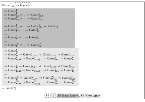
Figure 3 shows the order of our hybrid games.

Gamereal ⇒Game11

⇒Game12

⇒Game1₃_,₁⇒...⇒Game1₁₁_,₁

⇒Game1₃_,₂⇒...⇒Game1₁₁_,₂

...

⇒Game1₃_,r⇒...⇒Game1₁₁_,r⇒Game1₁₂

⇒Game2₁⇒...⇒Game2₁₂

...

⇒Gamei₁⇒...⇒Gamei₁₂

...

⇒GameQ1

1 ⇒...⇒Game

Q1

12

⇒Game113

⇒Game1₁₄⇒Game1₁₅_,₁...⇒Game1₁₅_,_{|U |}⇒Game1₁₅_,H

⇒Game1₁₆_,H ⇒Game1₁₆_,_{|U |}...⇒Game1₁₆_,₁⇒Game1₁₇

...

⇒Gamei14⇒Game

i

15,1...⇒Game

i

15,|U |⇒Game i

15,H

⇒Gamei₁₆_,H ⇒Gamei₁₆_,_{|U |}...⇒Gamei₁₆_,₁⇒Gamei₁₇

...

⇒GameQ2

14 ⇒Game

Q2

15,1...⇒Game

Q2

15,|U |⇒Game Q2

15,H

⇒GameQ2

16,H ⇒Game Q2

16,|U |...⇒Game Q2

16,1⇒Game

Q2

17

⇒GameQ2

18

SF-CT , SF-Keys-Before , SF-Keys-After

(16)

5.3 Hybrid Indistinguishability Lemmas

The following is a sequence of hybrid indistinguishability lemmas that will be combined at the end to form our adaptive security theorem.

Lemma 7. For any polynomial time adversary A, there exists a polynomial time B₁ such that

|Advreal(A, λ)−Adv11(A, λ)| ≤AdvSXDHG (B1, λ)

Proof. Given g, h, ga, gb andT =gab+r∗ ∈Gwhere eitherr∗= 0 or is a uniform random element of

Zp, consider the following simulator B1 in the security game:

First,B1 generates orthonormal bases:

(J,J∗)←Dual(Z6p)

(F,F∗)←Dual(Z3(pr+1))

(Ki,K∗i)←Dual(Z3p) for i∈ U

The bases (B,B∗) are implicitly defined as: ~b∗

i =f~

∗

i +a ~f

∗

r+1+i+a ~f

∗

2(r+1)+i fori∈[1, r]

~b∗

r+1 =f~

∗

r+1+as˜

0_~

f₂₍∗_r₊₁₎+a˜s00f~₃₍∗_r₊₁₎ ~b∗

i =f~i∗ for all otheri

~b₍_r₊₁₎₊_i =f~₍_r₊₁₎₊_i−a ~fi fori∈[1, r]

~b₂₍_r₊₁₎₊_i=f~2(r+1)+i−a ~fi fori∈[1, r]

~b2(r+1)=f~2(r+1)−as˜0f~(r+1)

~b₃₍_r₊₁₎=f~₃₍_r₊₁₎−as˜00f~₍_r₊₁₎ ~bi =f~i for all otheri

where ˜s0,˜s00←_Z_p are drawn byB₂ (and later used in the challenge ciphertext construction). (D,D∗)

are implicitly defined as:

~

d∗₂=~j₂∗+a~j₄∗+a~j₆∗ ~

d∗_i =~j_i∗ for all otheri

~

d4=~j4−a~j2

~

d6=~j6−a~j2

~

(17)

and (Ai,A∗i) are implicitly defined as:

~a∗_i,₁ =~k∗_i,₁+as˜0~k∗_i,₂+as˜00~k_i,∗₃ ~a∗_i,₂ =~k∗_i,₂

~a∗_i,₃ =~k∗_i,₃

~a_i,₁ =~k_i,₁

~a_i,₂ =~k_i,₂−as˜0~ki,1

~a_i,₃ =~k_i,₃−as˜00~ki,1

The public parameters are then generated by drawing ai←Zp fori∈ U and forming:

e(g, h)

(~e1)D∗,(~e2)D∗ {(~ei)B∗}i∈[r+1]

{(ai,0,0)A∗i}i∈[k]

Note that the terms in the public parameter can be generated since all vectors in the D∗,B∗,A∗i

bases are known directly except for d~∗₂,~b∗_i for i∈[r+ 1], and all~ai,1 and B1 can generate d∗2 by computing g~j2∗·₍_ga₎~j∗4 ₌_d∗

2,b∗i for i∈[r] by computing g ~

f_i∗_·₍_ga₎f~(∗r+1)+i _·₍_ga₎f~ ∗

2(r+1)+i ₌_b∗

i, and

a∗_i,₁ by computingg~ki,∗1_·₍_ga₎˜s0~k∗i,2 _·₍_ga₎s˜00~k∗i,2 ₌_a∗

i,1.

Similarly, note that all vectors inD,B,Aiare known explicitly except ford~4, ~d6,~b(r+1)+i,~b2(r+1)+i

for i∈[r+ 1], and~ai,2, ~ai,3 for i∈ U, but for normal secret keys ofT ype0, those entries are all 0. So,B1 is able to generate appropriately distributed secret keys of T ype0 for all secret key requests. For the challenge ciphertext request, let w~ be defined relative to the first requested secret key (this will be known upon ciphertext generation since this secret key is defined to be the first request before the challenge ciphertext request). Recall that the first coordinate of w~ is always 1. B1 draws

α,˜s,z˜i ←Zp fori∈[r] and constructs:

m·e(g, h)α,





α −(b) 0 −(ab+r) 0 −(ab+r)





J∗





(b) (b) + ˜z2 . . . (b) + ˜zr (b) + ˜s

(ab+r) (ab+r)w2+ (a)˜z2 . . . (ab+r)wr+ (a)˜zr (ab+r)˜s0+ (a)˜s0s˜

(ab+r) (ab+r)w2+ (a)˜z2 . . . (ab+r)wr+ (a)˜zr (ab+r)˜s00+ (a)˜s00s˜





F∗



 

  



−(b)ai−sa˜ i

−(ab+r)˜s0ai−(a)˜s0sa˜ i

−(ab+r)˜s00ai−(a)˜s0˜sai





K∗i



 

 

i∈S

which in the right bases, is:

m·e(g, h)α,





α −b

0 −r





D∗





b b+ ˜z2 . . . b+ ˜zr b+ ˜s

r ~w rs˜0

r ~w rs˜00





B∗



 

  



−(b+ ˜s)ai

−rs˜0ai

−rs˜00ai





A∗i



 

 

(18)

which is a properly distributed ciphertext of T ype0 when r = 0 where ∆ = b, s = b+ ˜s and

zi =b+ ˜zi, and is a properly distributed ciphertext of T ype1 when r← Zp where ∆ = b,∆0 =r,

s=b+ ˜s, s0 =rs˜0, s00=rs˜00, and zi=b+ ˜zi.

So, B₁ is able to exactly simulate Gamereal and Game11 when its SXDH challenge hasr = 0 and

r←_Z_p respectively. It then follows that for any difference inA’s advantage between the two games,

B1 can use A’s answers to achieve that same advantage in the SXDH game.

Lemma 8. For 1≤`≤Q1, for any polynomial time adversary A, there exists a polynomial time

B₂_,` such that

|Adv`₁(A, λ)−Adv`₂(A, λ)| ≤AdvSXDHG (B2,`, λ)

Proof. Giveng, h, ha, hb andT =hab+r∗ ∈Gwhere either r∗ = 0 or is a uniform random element of Zp, consider the following simulatorB2,` in the security game:

First,B₂_,`generates orthonormal bases:

(F,F∗)←Dual(Z3(p r+1))

(Ai,A∗i)←Dual(Z3p) for i∈ U

The bases (B,B∗) are implicitly defined as:

~bi =f~i+a ~f(r+1)+i fori∈[1, r]

~bi =f~i for all otheri

~b∗

(r+1)+i=f~

∗

(r+1)+i−a ~f

∗

i fori∈[1, r]

~b∗

(D,D∗) are implicitly defined as:

~

d2=~j2+a~j4

~

di=~ji for all otheri

~

d∗₄=~j₄∗−a~j₂∗ ~

e(g, h)

(~e1)D∗,(~e2)D∗ {(~ei)B∗}i∈[r+1]

{(ai,0,0)A∗i}i∈[k]

with nonzero components in the public parameters are known directly.

Similarly, note that all vectors in D,B,Ai are known explicitly except ford~2 and~bi fori∈[r]

and these can be constructed by takingh~j2_·₍_ha₎~j4 ₌_d

2, andhf~i·(ha)

~

f(r+1)+i ₌_b

(19)

B₂_,` is able to generate appropriately distributed secret keys ofT ype12 for all secret key requests before the`th key as well as keys of T ype0 for requests after the `th request.

For the challenge ciphertext request, let w~ be defined relative to the `th requested secret key (this will be known upon ciphertext generation since this secret key is defined to be one of the

Q1 requested before the challenge ciphertext). B2,` draws α,∆0, s, s0, s00,z˜i ← Zp for i ∈ [r] and

constructs:

m·e(g, h)α,





α 0

0 ∆0





J∗





0 z˜2 . . . z˜r s

∆0 ∆0w2 . . . ∆0wr s0

∆0 ∆0w2 . . . ∆0wr s00

  F∗        −sai

−s0ai

−s00ai





A∗i



 

 

i∈S

m·e(g, h)α,





α a∆0

0 ∆0





D∗





a∆0 a∆0w2+ ˜z2 . . . a∆0wr+ ˜zr s

∆0w~ s0

∆0w~ s00

  B∗        −sai

−s0ai

−s00ai





A∗i



 

 

i∈S

which is a properly distributed ciphertext of T ype1 =T ype2 where ∆ =a∆0, and zi=a∆0+ ˜zi.

For the `th key request,B2,` draws yj ←Zp forj ∈M and constructs:





1 (b)

0 (ab+r)

0 0   J                   

(b)M1,j (b)M2,j ... (b)Mr,j aρ(j)yj

(ab+r)M1,j (ab+r)M2,j ... (ab+r)Mr,j 0

0 0 ... ... 0

  F   yj 0 0  

Aρ(j)

                

j∈M

  1 b 0 r 0 0   D       

bM1,j bM2,j ... bMr,j aρ(j)yj

rM1,j rM2,j ... rMr,j 0

0 0 ... ... 0

  B   yj 0 0  

Aρ(j)



 

 

j∈M

which is a properly distributed secret key of T ype1 when r = 0 where x = b and is a properly distributed secret key ofT ype2 when r←Zp wherex=b and x0 =r.

So, B₂_,` is able to exactly simulate Game`₁ and Game`₂ when its SXDH challenge has r= 0 and

r←_Z_p respectively. It then follows that for any difference inA’s advantage between the two games,

(20)

For the connection to the following lemma, note that Game`₂ is equivalent to Game`₁₁_,₀.

Lemma 9. For 1≤`≤Q1, for 1≤k≤r, for any polynomial time adversary A, there exists a

polynomial time B₃_,k,` such that

|Adv`₁₁_,k−1(A, λ)−Adv`3,k(A, λ)| ≤AdvSXDHG (B3,k,`, λ)

Proof. Giveng, h, ha, hb andT =hab+r∗ ∈Gwhere either r∗ = 0 or is a uniform random element of Zp, consider the following simulatorB3,k,` in the security game:

First,B3,k,` generates orthonormal bases:

~br+1 =f~r+1+

r

X

i=1

a˜tif~(r+1)+i

~b₍_r₊₁₎₊_i =f~(r+1)+i+f~2(r+1)+i fori∈[1, r]

~bi =f~i for all other i

~b∗

(r+1)+i =f~

∗

(r+1)+i−a˜tif~

∗

r+1 fori∈[1, r]

~b∗

2(r+1)+i =f~

∗

2(r+1)+i−f~

∗

(r+1)+i+a˜tif~(∗r+1) fori∈[1, r]

~b∗

i =f~i∗ for all other i

where B₃_,k,` draws ˜ti ←Zp.

e(g, h)

(~e1)D∗,(~e2)D∗ {(~ei)B∗}i∈[r+1]

{(ai,0,0)A∗i}i∈[k]

Similarly, note that all vectors with nonzero components in T ype0 andT ype12 secret keys are

known explicitly except for~br+1 and this can be constructed by taking hf~r+1·

r

Y

i=1

(ha)t˜if~(r+1)+i ₌_b

i

fori∈[r]. So, B3,k,` is able to generate appropriately distributed secret keys of T ype12 for all secret key requests before the`th key as well as keys of T ype0 for requests after the `th request.

(21)

requested before the challenge ciphertext). B₃_,k,` draws α,∆,∆0, s, s0, s00, zi ← Zp for i∈ [r] and

constructs:

m·e(g, h)α,





α ∆

0 ∆0





D∗





∆ z2 . . . zr s

0 0 . . . 0 s0

∆0w~ s00

  F∗        −sai

−s0ai

−s00ai





A∗i



 

 

i∈S

m·e(g, h)α,





α ∆

0 ∆0





D∗





∆ z2 . . . zr s

∆0w~ s0

∆0w~ s00

  B∗        −sai

−s0ai

−s00ai





A∗i



 

 

i∈S

which is a properly distributed ciphertext of T ype2 =T ype3,k =T ype11,k−1.

For the `th key request,B₃_,k,` draws x, x0, x∗, yj ←Zp forj∈M and constructs:





1 x

0 x0

0 0   J       

x∗M1,j+aρ(j)yjt˜1(a) x∗M2,j+aρ(j)yj˜t2(a) ... x∗Mr,j+aρ(j)yj˜tr(a) 0

x∗M1,j x∗M2,j ... x∗Mr,j 0

  F   yj 0 0  

Aρ(j)



 

 

j<k∈M

∪       

x0M1,j+aρ(j)yjt˜1(a) x0M2,j+aρ(j)yj˜t2(a) ... x0Mr,j+aρ(j)yj˜tr(a) 0

x0M1,j x0M2,j ... x0Mr,j 0

  F   yj 0 0  

Aρ(j)



 

 

j>k∈M

∪       

xM1,k xM2,k ... xMr,k aρ(k)(b)

x0M1,k+aρ(k)˜t1(ab+r) x0M2,k+aρ(k)˜t2(ab+r) ... x0Mr,k+aρ(k)˜tr(ab+r) 0

x0M1,k x0M2,k ... x0Mr,k 0





F





(b) 0 0





Aρ(k)



 

 





1 x

0 x0

0 0   D       

x∗M1,j x∗M2,j ... x∗Mr,j 0

0 0 ... ... 0

  B   yj 0 0  

Aρ(j)



 

 

(22)

∪ 

 

  



x0M1,j x0M2,j ... x0Mr,j 0

0 0 ... ... 0





B





yj

0 0





Aρ(j)



 

 

j>k∈M

∪ 

 

  



xM1,k xM2,k ... xMr,k aρ(k)b

x0M1,k+ ˜t1raρ(k) x0M2,k+ ˜t2raρ(k) ... x0Mr,k+ ˜trraρ(k) 0

−˜_t₁_ra_ρ₍_k₎ ˜_t₂_ra_ρ₍_k₎ _... −˜_t_r_ra_ρ₍_k₎ ₀





B





b

0 0





Aρ(k)



 

 

which is a properly distributed secret key of T ype11,k−1 when r= 0 where yk=b and is a properly

distributed secret key ofT ype3,k whenr ←Zp where yk=b andti = ˜tiraρ(k).

So, B₃_,k,` is able to exactly simulate Game`₁₁_,k₋₁ and Game`₃_,k when its SXDH challenge has

r= 0 and r ←Zp respectively. It then follows that for any difference inA’s advantage between the

two games, B₃_,k,` can useA’s answers to achieve that same advantage in the SXDH game.

polynomial time B₄_,k,` such that:

|Adv`₃_,k(A, λ)−Adv`₄_,k(A, λ)| ≤AdvSXDHG (B4,k,`, λ)

Proof. Looking at theK2,k, K3,k components of the Type3,k `th key (the ones containing the ti and

the only things that differ in definition between Game`₃_,k and Game`₄_,k):





x0M1,k+t1 x0M2,k+t2 ... x0Mr,k+tr 0

−t1 −t2 ... −tr 0





B





yk

0 0





Aρ(k)

we see that this is identically distributed to:





−˜_t₁ −˜_t₂ _... −˜_t_r ₀

x0M1,k+ ˜t1 x0M2,k+ ˜t2 ... x0Mr,k+ ˜tr 0





B





yk

0 0





Aρ(k)

where implicitly ˜ti=−xM1,k−ti.

So, the transition from Type3,k key to Type4,k is symmetric to the one from Type11,k−1 to Type3,k, and by applying the simulation from Lemma9 accordingly (flipping the embeddings of

the bottom two rows ofB,B∗), B4,k,` could use A’s answers to achieve the same advantage in the

SXDH game.

polynomial time B₅_,k,` such that:

|Adv`₄_,k(A, λ)−Adv`₅_,k(A, λ)| ≤AdvSXDHG (B5,k,`, λ)

Proof. Giveng, h, ha_{, h}b _and_T ₌_hab+r∗ _∈_G_{where either} _r∗ _{= 0 or is a uniform random element}

(23)

First,B₅_,k,` generates orthonormal bases:

~b(r+1)=f~(r+1)+a ~f3(r+1)

~bi=f~i for all otheri

~b∗

3(r+1)=f~

∗

3(r+1)−a ~f

∗

(r+1)

~b∗

(Ai,A∗i) are implicitly defined as:

~a1,i =~k1,i+a~k3,i

~a2,i =~k2,i

~a3,i =~k3,i

~a∗₁_,i =~k₁∗_,i ~a∗₂_,i =~k₂∗_,i

~a∗₃_,i =~k₃∗_,i−a~k∗₁_,i

e(g, h)

(~e1)D∗,(~e2)D∗ {(~ei)B∗}i∈[r+1]

{(ai,0,0)A∗i}i∈[k]

Similarly, note that all vectors with nonzero components in T ype0 andT ype12 secret keys are known explicitly except for~br+1and this can be constructed by takinghf~r+1·(ha)

~

f3(r+1) ₌_b

(r+1). So,

B₅_,k,` is able to generate appropriately distributed secret keys of T ype12 for all secret key requests before the`th key as well as keys of T ype0 for requests after the `th request.

Q1 requested before the challenge ciphertext). B5,k,` drawsα,∆,∆0, s0, s00, zi ←Zp for i∈[r] and

constructs:

m·e(g, h)α,





α ∆

0 ∆0





D∗





∆ z2 . . . zr 0

∆0w~ s0

∆0w~ s00





F∗



 

  



0

−s0ai

−s00ai





K∗i



 

 

(24)

m·e(g, h)α,





α ∆

0 ∆0





D∗





∆ z2 . . . zr as00

∆0w~ s0

∆0w~ s00

  B∗        −as00ai

−s0ai

−s00ai





A∗i



 

 

i∈S

which is a properly distributed ciphertext of T ype2 =T ype4,k =T ype5,k where s=as00.

For the `th key request,B₅_,k,` draws x, x0, x∗, yj ←Zp forj∈M and constructs:





1 x

0 x0

0 0   D       

x∗M1,j x∗M2,j ... x∗Mr,j 0

0 0 ... ... a_ρ₍_j₎yj(a)

  F   yj 0

yj(a)





Kρ(j)



 

 

j<k∈M

∪       

x0M1,j x0M2,j ... x0Mr,j 0

0 0 ... ... a_ρ₍_j₎yj(a)

  F   yj 0

yj(a)





Kρ(j)



 

 

j>k∈M

∪       

xM1,k xM2,k ... xMr,k aρ(k)(b)

0 0 ... 0 0

x0M1,k x0M2,k ... x0Mr,k aρ(k)(ab+r)





F





(b) 0 (ab+r)





Kρ(k)



 

 





1 x

0 x0

0 0   D       

x∗M1,j x∗M2,j ... x∗Mr,j 0

0 0 ... ... 0

  B   yj 0 0  

Aρ(j)



 

 

j<k∈M

∪       

x0M1,j x0M2,j ... x0Mr,j 0

0 0 ... ... 0

  B   yj 0 0  

Aρ(j)



 

 

j>k∈M

∪       

xM1,k xM2,k ... xMr,k aρ(k)b

0 0 ... 0 0

x0M1,k x0M2,k ... x0Mr,k aρ(k)r

  B   b 0 r  

Aρ(k)



 

 

which is a properly distributed secret key of T ype4,k when r = 0 where yk =band is a properly

(25)

So, B₅_,k,` is able to exactly simulate Game`₄_,k and Game`₅_,k when its SXDH challenge hasr= 0 andr←_Z_p respectively. It then follows that for any difference inA’s advantage between the two games, B5,k,` can useA’s answers to achieve that same advantage in the SXDH game.

Lemma 12. For 1≤`≤Q1, for 1≤k≤r, for any adversary A,

|Adv`₅_,k(A, λ)−Adv`₆_,k(A, λ)|= 0

Proof. Given the bases:

Define the bases (B,B∗) as:

~b₃₍_r₊₁₎ = ˜a ~f3(r+1)

~bi=f~i for all other i

~b∗

3(r+1) = ˜a

−1_f_~∗

3(r+1)

~b∗

i =f~

∗

i for all other i

for a random ˜a←_Z_p, define (Ai,A∗i) as equal to (Ki,K∗i) for i=ρ(k) and define (Ai,A∗i) as:

~a1,i=~k1,i

~a2,i=~k2,i

~a3,i= ˜a~k3,i

~a∗₁_,i=~k∗₁_,i ~a∗₂_,i=~k∗₂_,i ~a∗₃_,i= ˜a−1~k₃∗_,i

fori6=ρ(k).

Consider simulating Game`₅_,k with the (D,D∗),(B,B∗),(Ai,A∗i) bases. We will see that doing

so is equivalent to simulating Game`₆_,k with the (D,D∗),(F,F∗),(Ki,K∗i) bases. Since both sets of

bases come from the same distribution, then the two games are identical.

The only key-side elements that have a non-zero component in a vector that has been transformed between the two bases are the K2,k, K3,k components of the (simulated Type5,k) `th key:



 

  



0 0 ... 0 0

x0M1,k x0M2,k ... x0Mr,k aρ(k)yk0





B





yk

0

y_k0





Aρ(k)



 

(26)

which in the (D,D∗),(F,F∗),(Ki,K∗i) looks like:       

0 0 ... 0 0

x0M1,k x0M2,k ... x0Mr,k aρ(k)˜ay0k

  F   yk 0

y_k0





Kρ(k)



 

 

a properly distributed Type6,k key where ˜aρ(k)= ˜aaρ(k).

The only ciphertext-side elements that have a non-zero component in a vector that has been transformed between the two bases are theC2,k, K3,kcomponents of the (simulated Type5,k) challenge

ciphertext:

m·e(g, h)α,





α ∆

0 ∆0





D∗





∆ z2 . . . zr s

∆0w~ s0

∆0w~ s˜00

  B∗        −sai

−s0ai

−˜s00ai





A∗i



 

 

i∈S

which in the (D,D∗),(F,F∗),(Ki,K∗i) looks like:

m·e(g, h)α,





α ∆

0 ∆0





D∗





∆ z2 . . . zr s

∆0w~ s0

∆0w~ s˜00˜a−1

  F∗        −sai

−s0ai

−s˜00a˜−1_a

i





K∗i



 

 

i6=ρ(k)∈S

[       

−sai

−s0ai

−(˜s00˜a−1_)(˜_aa

i)





K∗i



 

 

i=ρ(k)∈S

which is a properly distributed Type6,k challenge ciphertext where s00= ˜s00a˜−1, ˜aρ(k)=aρ(k)a˜. These are the only elements that interact with the transformed basis vectors during the simulation, the transformation results in the same distribution of basis vectors, and we showed the using one set simulates Game`₅_,k and using the other simulates Game`₆_,k, therefore the two games are identical and no adversary can achieve a difference in advantage between the two.

|Adv`₆_,k(A, λ)−Adv`₇_,k(A, λ)|= 0

Proof. This follows from a direct application of Lemma 8 from [Tak17] (which relies on Lemma 3 from [OT10]). Essentially, the lemma says that since the only nonzero elements in the third row of the (B,B∗) basis are in the single challenge ciphertext and the `th key’skth componentsK2,k, then

their distribution is dependent only on their dot product. We reproduce the lemma in AppendixA’s

Lemma31.

If aρ(k) ∈ S for the challenge ciphertext, then we have that w~ ·M~k = w~ ·x0M~k = 0. So, by

Lemma 31 we can switch x0M~k to x∗M~k in the `th key’s kth component without changing the

distribution, since w~ ·x∗M~k= 0.

Ifaρ(k)6∈S for the challenge ciphertext, then we know that ˜aρk appears only in the `th key’s kth

component. So, we can use the same lemma to argue that its randomness blinds the dot product. Specifically, we look at the dot product of the previous vectors plus the additional 3(r + 1)th component, which is equal to: w~·x0M~k+s00a˜ρ(k), which is uniformly random because of the presence of ˜aρ(k). So, again by Lemma 31, we can switch x0M~k to x∗M~k in the `th key’s kth component

(27)

|Adv`₇_,k(A, λ)−Adv`₈_,k(A, λ)|= 0

polynomial time B₉_,k,` such that:

|Adv`₈_,k(A, λ)−Adv`₉_,k(A, λ)| ≤AdvSXDHG (B9,k,`, λ)

polynomial time B₁₀_,k,` such that:

|Adv`₉_,k(A, λ)−Adv`₁₀_,k(A, λ)| ≤AdvSXDHG (B10,k,`, λ)

polynomial time B11,k,` such that:

|Adv`₁₀_,k(A, λ)−Adv`₁₁_,k(A, λ)| ≤AdvSXDH_G (B₁₁_,k,`, λ)

Proof. These proofs follow the same arguments as Lemma12, Lemma11, Lemma10, and Lemma9

respectively, in reverse, and usingx∗ instead ofx0 in the `th key’s kth component.

Lemma 18. For 1≤`≤Q1, for any polynomial time adversary A, there exists a polynomial time

B12,` such that:

|Adv`₁₁_,r(A, λ)−Adv`₁₂(A, λ)| ≤AdvSXDHG (B12,`, λ)

Proof. This lemma is almost essentially a reverse of Lemma 8 using x∗ instead of x0, except the

x0 in the Dbasis of the`th key is not removed. So, we will show that we can fix it so it does not

disappear when the rest of the x∗ components go to 0:

Given g, h, ha, hb andT =hab+r∗ ∈Gwhere either r∗= 0 or is a uniform random element of Zp,

consider the following simulatorB₁₂_,` in the security game:

First,B12,` generates orthonormal bases:

~bi =f~i+a ~f(r+1)+i fori∈[1, r]

~bi =f~i for all otheri

~b∗

(r+1)+i=f~

∗

(r+1)+i−a ~f

∗

i fori∈[1, r]

~b∗

i =f~

∗

(28)

(D,D∗) are implicitly defined as:

~

d2=~j2+a~j4

~

di=~ji for all otheri

~

d∗₄=~j₄∗−a~j₂∗ ~

e(g, h) (~e1)D∗,(~e2)D∗ {(~ei)B∗}i∈[r+1]

{(ai,0,0)A∗i}i∈[k]

Similarly, note that all vectors in D,B,Ai are known explicitly except ford~2 and~bi fori∈[r]

and these can be constructed by takingh~j2_·₍_ha₎~j4 ₌_d

2, andhf~i·(ha)

~

f(r+1)+i ₌_b

i fori∈[r]. So,

B₁₂_,` is able to generate appropriately distributed secret keys ofT ype0 for all secret key requests before the`th key as well as keys of T ype12 for requests after the`th request.

Q1 requested before the challenge ciphertext). B12,` draws α,∆0, s, s0, s00,z˜i ←Zp for i ∈[r] and

constructs:

m·e(g, h)α,





α 0

0 ∆0





J∗





0 z˜2 . . . z˜r s

∆0 ∆0w2 . . . ∆0wr s0

∆0 ∆0w2 . . . ∆0wr s00





F∗



 

  

 −sai

−s0ai

−s00ai





A∗i



 

 

i∈S

m·e(g, h)α,





α a∆0

0 ∆0





D∗





a∆0 a∆0w2+ ˜z2 . . . a∆0wr+ ˜zr s

∆0w~ s0

∆0w~ s00





B∗



 

  

 −sai

−s0ai

−s00ai





A∗i



 

 

i∈S

which is a properly distributed ciphertext of T ype1 =T ype2 where ∆ =a∆0, and zi=a∆0+ ˜zi.

For the `th key request,B12,` draws ˜x0, yj ←Zp forj ∈M and constructs:





1 (b)

0 (ab+r) + ˜x0

0 0



