Modeling of air-gap membrane distillation process: a theoretical and experimental study

1

Modeling of air-gap membrane distillation process: A

theoretical and experimental study

A.S. Alsaadi

,

N. Ghaffour

, J.-D. Li

, S. Gray

, L. Francis

, H. Maab

, G.L. Amy

a_{Water Desalination and Reuse Center, King Abdullah University of Science and Technology (KAUST),}

23955-6900 Thuwal, Saudi Arabia, Tel. +966-28082180, Email: [email protected]

b

School of Engineering and Science, Victoria University, P.O. Box 14428, Melbourne, Victoria 8001, Australia

c_{Institute of Sustainability and Innovation, Victoria University, P.O. Box 14428, Melbourne, Victoria 8001,}

Australia

Abstract

A one dimensional (1-D) air gap membrane distillation (AGMD) model for flat sheet type

modules has been developed. This model is based on mathematical equations that describe the

heat and mass transfer mechanisms of a single-stage AGMD process. It can simulate AGMD

modules in both co-current and counter-current flow regimes. The theoretical model was

validated using AGMD experimental data obtained under different operating conditions and

parameters. The predicted water vapor flux was compared to the flux measured at five different

feed water temperatures, two different feed water salinities, three different air gap widths and

two MD membranes with different average pore sizes. This comparison showed that the model

flux predictions are strongly correlated with the experimental data, with model predictions being

within +10% of the experimentally determined values. The model was then used to study and

analyze the parameters that have significant effect on scaling-up the AGMD process such as the

effect of increasing the membrane length, and feed and coolant flow rates. The model was also

used to analyze the maximum thermal efficiency of the AGMD process by tracing changes in

water production rate and the heat input to the process along the membrane length. This was

used to understand the gain in both process production and thermal efficiencyfor different

membrane surface areas and the resultant increases in process capital and water unit cost.

Keywords: Air-gap membrane distillation (AGMD); Modeling; Thermal efficiency; Co-current

2

1. Introduction

Membrane Distillation (MD) is a thermally driven separation process that utilizes a

hydrophobic, micro-porous membrane as a contactor between two fluids maintained at different

temperatures where the separation is achieved by the mass transfer of the vapor phase. At

relatively low operating pressures the hydrophobicity of the micro-porous membrane prevents

the liquid phase from wetting the membrane pores and vapor is the only phase to pass through

the membrane. The difference in fluid temperatures between the two sides of the membrane

creates a driving force for the vapor to pass from the fluid at higher temperature (feed) to the one

at lower temperature (coolant).

MD holds high potential for several applications including water desalination [1]. It is an

alternative sustainable technology that can be driven by solar, geothermal or waste heat [2]. One

of the main advantages of MD is that process performance is not highly affected by high feed

salinity, as was proven in bench scale [3,4] and in full scale [5] studies.

Air Gap Membrane Distillation (AGMD) is one of the four common MD configurations. It is

characterised by the presence of a stagnant air gap between the membrane and the condensation

surface to reduce the heat loss by conduction. Because of the improved thermal efficiency of

AGMD compared to direct contact membrane distillation (DCMD), it became the first choice for

pilot testing to address scale-up and long-term operational issues [5-9]. This may be due to the

close similarity of the AGMD configuration to the matured Multi-Stage Flash (MSF) technology.

The former technology can be described as an intensification of the latter one. In other words,

even though the two technologies share many similar features, AGMD is reduced in size

compared to MSF, because of its higher surface area to volume ratio, and can possibly achieve

the same level of production and thermal efficiency. Furthermore, it holds future potential

advantages over the conventional thermal-based processes such as:

- It can be decentralized since it is modular and any low grade heat source (solar energy,

waste-heat) can be sufficient for its operation.

- AGMD modules can be made of inexpensive polymeric materials that are corrosion

resistant.

- As is the case with most membrane-based separation technologies, the MD operation

3 - Low operation and maintenance cost and no chemicals required [11].

Modeling of AGMD processes has generally taken either of two approaches: 0-dimentional

modeling (0-D) where the transport of heat and mass are averaged over the module, and

two-dimensional modeling (2-D) where variations in heat and mass transfer conditions along the

membrane are taken into consideration (i.e., temperature profiles, hydrodynamics). The

limitations of these approaches are:

- 0-D models [12-20]: these models do not consider the changes of the fluid conditions as

they flow inside the AGMD module. Averaged fluids properties are used as inputs to these

models. Such models do not account for changes in temperature (and therefore driving

force) along the membrane length, and process scale-up can only be predicted from

experiments using an AGMD module of the same dimensions and identical operating

conditions (i.e., pilot plant trials). Therefore, this approach can neither be used for

optimization nor can it predict performance from small scale laboratory experiments or

conditions for which experiments have not been conducted.

- 2-D models [21-24]: these models involve detailed computational fluid dynamic (CFD)

simulation of the flow parameters and heat transfer across a 2-dimentional membrane

surface. Such models are computationally intensive and require longer time to achieve

results, especially for large membrane surface areas. Given that the configuration of most

AGMD systems are flat sheet membranes where the conditions are assumed to be identical

across the membrane width, the extra complication of 2-D modeling compared to

1-dimentional modeling (1-D) appears unnecessary.

To the authors’ knowledge, there has been only one 1-D model for AGMD reported in the

literature to date, although 1-D modeling of DCMD has become established [25-28]. Guijt et al.

[29] developed a 1-D model for a single hollow fiber module using the Dusty gas model and

considered counter-current flow only. In this paper, a 1-D AGMD model for a flat sheet module

was developed for both co-current and counter-current flow regimes. The theoretical model

predictions were validated and compared with experimental results obtained using a locally

designed and fabricated AGMD module and commercially available PTFE membranes of two

different pore sizes.

4 The 1-D AGMD mathematical model developed was for flat sheet membranes typically used

in commercial MD pilot units. The model is based on dividing the AGMD module longitudinally

into small elements. Within each element, different zones exist where significant mass and

energy exchange occurs along the boundaries of these zones. As depicted in Figure 1, the zones,

in order from left to right, are as follows:

- The hot fluid channel

- The polymeric membrane layer

- The air gap space

- The condensate film on the cooling plate

- The cooling plate sheet

- The cold fluid channel

Figure 1: A schematic diagram of AGMD longitudinal zones used in describing the model.

In Figure 1, it is assumed that flow direction, x, is the same as that of the hot feed flow, and

each small element is assumed to have a length of dx and a constant width W. Moreover, the

mathematical model calculations were simplified according to the following assumptions:

1. The system is at steady state condition.

2. The hot and cold fluids are assumed to flow in the x direction only.

3. The pressure inside the air gap is constant (no pressure drop along the air gap zone).

4. The condensation on the cooling plate is film-wise and the thickness of the falling film

inside the air gap is small in comparison with the width of the air gap.

5. Within the air gap, there is no bulk velocity of the air-vapor mixture. Heat is transferred

by conduction while mass is transferred through diffusion.

6. Pure water vapor is only transported through membrane pores.

7. There is no heat being exchanged with the surrounding.

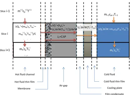
A magnification of two consecutive slices to illustrate the exchange of mass and heat is

shown in Figure 2.

5 The mass and energy balances of slice i in the hot fluid channel can be described as follows:

∆𝑚ℎ𝑖 = 𝑚ℎ𝑏𝑖− 𝑚ℎ𝑏𝑖−1 (1)

𝑚ℎ𝑏𝑖𝑆𝑖 = 𝑚ℎ𝑏𝑖−1𝑆𝑖−1 (2)

𝑄ℎ𝑖𝑑𝑥𝑖𝑊 =𝑚ℎ𝑏𝑖𝑐𝑝ℎ𝑏𝑖𝑇ℎ𝑏𝑖− 𝑚ℎ𝑏𝑖−1𝑐𝑝ℎ𝑏𝑖−1𝑇ℎ𝑏𝑖−1 (3)

where ∆mhi is the change in the hot feed mass flow rate of slice i, mhbi, Si, mhbi-1 and Si-1 are the

hot feed mass flow rates and salt mass fractions exiting and entering slice i, respectively, Qhi is

the hot feed heat flux of slices i,cphbi, Thbi, cphbi-1 and Thbi-1 are the specific heat and bulk

temperature of the hot feed exiting and entering slice i, respectively.

The boundary layer was assumed to be a fully developed and transfers the mass that it

receives from the hot fluid channel slice through convection to the membrane layer as

compensation for the mass lost through evaporation.

∆𝑚ℎ𝑏𝑖 = 𝐽𝑣𝑖𝑑𝑥𝑖𝑊 (4)

where Jvi is the mass flux of the water vapor and W is the width of the flat sheet module. Heat is

also transferred by conduction in this slice from the hot fluid channel to the membrane layer

according to the following equation:

∆𝑄ℎ𝑖 =𝐻ℎ𝑖(𝑇ℎ𝑏𝑖− 𝑇ℎ𝑚𝑖) (5)

The heat transfer coefficient Hhican be calculated from the following correlation:

𝐻

=

where Nu is Nusselt’s number, kl is the hot fluid thermal conductivity and dh is the hydraulic

diameter of the hot channel. For a spacer filled channel, although the Reynolds number (Re) is

generally less than 300, Zhang et al. [28] suggest that model predictions fit experimental data

more accurately when the streams are assumed to be fully developed turbulent flow for the

calculation of Nu. Thus, Nu can be calculated from the following correlation after correcting for

the spacer effect by Ks.

0.8 0.33 0.029 _s

Nu= K Re Pr (7)

0.086 0.039 0.75

1.904( ) sin 2

f

s s

s d K

h

θ ε

−  

= _{ }

6 Where Pr is Prandtl number, dfis the spacer filament diameter, hs is the spacer thickness, εs is

the spacer porosity and θ is the angle that filaments make when they cross each other.

The spacer porosity can be calculated as follow:

1

s

total

V

V

ε

= −

(9)

where Vfilament and Vtotal are the volume of the filament and the whole spacer, respectively.

The local Re number in equation (7)can be computedfrom:

µ ρd_hV

=

Re (10)

where ρ, V, µ are the density, velocity and viscosity of the hot fluid in spacer-filled channel,

respectively, and dh is the hydraulic diameter of a spacer filled channel. The hydraulic diameter

for a single sized filament of rhombus mesh spacer can be calculated by [30]:

4.0

2 4(1- )

s f s

h

f s s

d h d

d h

ε ε

= +

(11)

The same calculations are applied for the heat transfer coefficient of the flow in the cold

channel. Furthermore, at steady state, the change in heat flux of the hot feed (Qih) and the change

in heat flux of the coolant (Qic) are equal and can be referred to as simply Qi. However, the mass

flow rate of the coolant is constant but that of the hot feed decreases because it loses water vapor

through the membrane (permeate) as it flows down the module. The following equation can be

used to quantify the amount of vapor that passes through the membrane pores:

) ' '

( hm ma

v C P P

J = − (12)

where C is the membrane mass transfer coefficient, P’hm is the saturation pressure of water at

Thm, P’ma is the partial pressure of water vapor at the interface between the membrane and the air

gap.

In calculating the mass transfer coefficient, Zhang et al. [28] concluded that, for DCMD, the

Knudsen-molecular diffusion is the dominating mass transfer mechanism within the pores of the

7

kv mv

v J J

J

1 1 1 _{= +}

(13)

where Jmv and Jkv are the vapor fluxes due to molecular diffusion and Knudsen diffusion,

respectively. In other words, the total membrane resistance to water vapor can be written as a

combination of two mass transfer resistances in series according to the following equation:

𝑅𝑣 = 𝑅𝑚𝑣+𝑅𝑘𝑣 (14)

where Rmv is the mass transfer resistance exerted by all non-condensable gases within the

membrane pores on the water vapor molecules, and Rkv is the mass transfer resistance due to the

momentum loss during the collision of water vapor molecule with the internal walls of the

membrane pores. When there are no non-condensable gases within the membrane pores the

resistance of Rmv becomes nil and the water vapor mass flux is mainly controlled by Knudsen

diffusion mechanism. At high partial pressure of non-condensable gases within the membrane

pores, the mass transfer is mainly controlled by molecular diffusion mechanism. The Knudsen

and molecular diffusions can be calculated through the following equations [28]:

) ' ' ( 1 ) ' ' ( 2 3 4 ma hm AB v mv ma hm v kv P P bRT D y M J P P RT M b d J − − = − = τ ε π τ ε (15)

where d, b, τ,ε are the average diameter of pores, the membrane thickness, the tortuosity of the

pores and the porosity of the membrane, respectively. Mv is the molecular weight of water, R is

the universal gas constant, and y is the mole fraction of water vapor in the membrane pores.

The mass diffusivity between the air and water vapor is given by [31]:

P T D_AB 072 . 2 5 10 895 .

1 × − =

(16)

where T is the average temperature and P is the total pressure. The mole fraction of water vapor

is related to vapor pressure Pv as:

P P

y = v

(17)

Combining equations 13, and 15-17 yields:

) ' ' ( ) ( 4 2 685 . 5 81 .

7 1.072

ma hm v v

v

v P P

8 Therefore, ) ( 4 2 685 . 5 . 81 .

7 1.072

v v v P P dR T RM T M b d C − + = π τ ε (19)

The total heat flux across the membrane can be calculated as:

g v ma

hm T J h

T b k

Qi = ₍ i − i₎+ i ₍₂₀₎

where hg is the enthalpy of the water vapor. The average thermal conductivity of the membrane

is calculated by:

m

air k

k

k=ε +(1−ε) (21)

where kair and km are the thermal conductivities of the air and the membrane material,

respectively. In equation (20), the first term is the sensible heat transfer through conduction and

the second term is the latent heat transfer of water.

For a small mole fraction of water vapor within the air gap channel, the mass transfer of the

water vapor can be approximately determined by [32]:

) ( _mai _fi

i

a AB i

v y y

cD

J = −

δ (22)

where 𝐽̅_𝑣𝑖is the molar flux of water vapor and is related to Jviby the molar mass of water vapor,

c is the total molar concentration, δa is the air gap width, DABi is the diffusivity coefficient, ymai is

the mole fraction of water vapor at Tmai and yfi is the mole fraction of water vapor at the interface

of the falling film and is a function of the saturation pressure of the water at Tfi.

The heat transfer within the air gap can be calculated by:

i g i v i f i ma a i AB i h J T T k

Q = ( − )+

δ (23)

where kABi is the thermal conductivity of the gas mixture of air and water vapor and i g

h is the

molar enthalpy of water vapor.

For the falling film, the model of Nusselt film condensation on a vertical plate is used [33].

The condensate film thickness in that model is determined by:

i v i i f i i f i av i l i l i i J dx d g dx

dm ₌ − δ ₌

9 where dmi /dxi is the rate of mass increase of the falling film in slice i and this should be equal

to the mass transfer of the water vapor Jvi, ρli is the density of water liquid, ρavi is the density of

the gas mixture, δf is the thickness of the falling film, g is the gravity acceleration, and µi is the

dynamic viscosity of the water liquid.

The heat transfer across the falling film is simply computed from:

) ( _fi _fwi

i f

i f i

T T k

Q = −

δ (25)

where kfi is the thermal conductivity of the water liquid film on the cooling plate. The heat

transfer across the coolant wall can be calculated as:

) ( _fwi _cwi

c i w i

T T k

Q = −

δ (26)

where kwi is the thermal conductivity of the cooling plate. For the coolant channel (the wall

bounding the coolant channel to the right shown in Figure 1 is assumed to be solid and

adiabatic), the energy balance gives:

𝑄𝑖_𝑑𝑥𝑖_{𝑊 =𝑚}

𝑐𝑖(𝑐𝑝𝑐𝑏𝑖𝑇𝑐𝑏𝑖− 𝑐𝑝𝑐𝑏𝑖−1𝑇𝑐𝑏𝑖−1) (27)

where mc and cpcb are the mass flow rate and specific heat of the coolant.

Also, the heat transfer in the coolant channel can be calculated as:

) ( _cwi _cbi

i c i

T T H

Q = − (28)

where Hci is the convective heat transfer coefficient of the coolant channel.

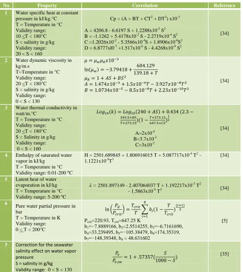
To correct for changes in the fluid conditions as they flow through the AGMD module the

correlation equations for the thermal properties presented in Table 1were used.

Table 1: Correlation equations of seawater physical properties.

2.1.Solution procedure

The solution to the co-current and counter-current regimes begins by re-arranging equation

(12) to take the following form:

ma hm

v _{P P}

C J

' ' −

= (29)

10 ) ' ' ( ) ( P P P P M cD y y M cD J M J i f i ma a v i AB i f i ma a v i AB i v i v i

v = = δ − = δ −

(30)

Since ρ = cMv then the mass flux becomes:

) ' ' ( ) ' '

( _mai _fi

m a v i AB i f i ma m a v i AB m

v P P

P M M D P P PM M D cM

J = − = −

δ ρ δ

(31)

Using the ideal gas law we get:

) ' ' ( ) ' '

( _mai _fi _mai _fi

i avg u a v i AB

v P P A P P

T R

M D

J = − = −

δ (32) i avg a v i AB i T R M D A δ = (33)

From Equation (32), we obtain:

f ma i

i

v _{P P}

A J

' ' −

= (34)

Combining Equations (29) and (34) gives:

) ' ( ) 1 1 ( ' ' ) 1 1 ( ' 1 i f i hm i i i v i f i hm i v i i P P A C J P P J A C − + = − = + − (35)

where P’hm and P’f are the saturation pressures at the corresponding temperatures.

From Equations (5), (20), (23) we get:

i f i ma i a i AB i g i v i i ma i hm i m i i g i v i i hm i hb i h i T T k h J Q T T k h J Q T T H Q − = − − = − − = δ δ / / (36)

Combining the three equations above, we get:

i f i hb i a i AB i g i v i i m i i g v i i h i

T

T

k

h

J

Q

k

h

J

Q

H

Q

₊

−

₊

−

₌

₋

δ

δ

/

/

11 i cb i cw i c i i cw i fw i c i w i i fw i f i f i f i T T H Q T T k Q T T k Q − = − = − = δ δ / / (38)

Combining the three equations of (38) results in:

i cb i f i c i c i w i f i f i T T H k k

Q + + 1 )= −

/ 1 / 1 ( δ

δ ₍₃₉₎

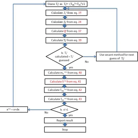
For co-current flow, the calculation starts by estimating Tfi where the mass flux (Jvi) can be

calculated from equation (35), the mass flux is then used in equations (24) and (37) to calculate the film thickness of the condensate (δfi) and Qi, respectively. At steady state, Qi in equations

(37) and (39) are equal. Therefore, equation (39) is used to re-calculate Tfi. The above steps can

be repeated until convergence. After the convergence of Tfi, the feed flow rate and its bulk

temperature and the temperature of the coolant of the next slice can be calculated from

W dx J m

m_hi+1= _hi− _vi i (40)

𝑆𝑖+1₌ 𝑚ℎ𝑏𝑖𝑆𝑖

𝑚ℎ𝑏𝑖+1 (41)

1

1 ( )

+ + ₌ + i h i hb i hb i hb i h i i i hb m Cp T Cp m W dx Q

T (42)

i c i cb i i i cb i cb m Cp W dx Q T

T +1 = + (43)

In the above equations, i+1 means the position of xi+1. The above procedures can be

performed from x =0 to x = L (the length of the module). However, for counter-current flow, the

solution is complicated by not knowing the exit temperature of the coolant fluid at x=0. Thus, the

exit temperature of the coolant should be estimated first. Since the coolant exit temperature is

always expected to be between the coolant inlet temperature and the inlet hot feed temperature,

the average of these temperatures can be used as an initial estimate of the coolant exit

temperature. The same co-current procedure is then used to calculate the inlet temperature of the

coolant except that the equations 40, 42 and 43 are changed into the following equations:

W dx J m

12

1

1 ( )

+

+ ₌ +

i h i hb

i hb i hb i h i

i i

hb

m Cp

T Cp m W dx Q

T (45)

i c i cb

i i i cb i cb

m Cp

W dx Q T

T +1= − (46)

The calculation is terminated when the estimation of the coolant exit temperature results in a

difference between the calculated coolant inlet temperature and the coolant inlet temperature

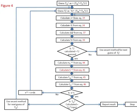
used as an input for the model calculation was below a pre-specified tolerance (0.001⁰C). Figures 3 and 4 show the algorithms used for the solution procedures in both flow regimes.

Figure 3: Calculation algorithm of the co-current flow model.

Figure 4:Calculation algorithm of the counter-current flow model.

3. Materials and methods

3.1.Experimental setup and membranes

Two commercially available hydrophobic micro-porous polytetrafluoroethylene (PTFE)

membranes with different mean (average) pore sizes (0.2 µm and 0.45 µm) provided by

Sterlitech Corporation were tested in the AGMD process. The porosity and thickness of both

membranes are 80 % and 100 µm each, respectively. Figure 5 shows the Scanning Electron

Microscopy (SEM) of these membranes and its contact angle. These data were used in Eq. (18)

to calculate the membrane mass transfer coefficient. A tortuosity of 1.5 for the pore structure was

assumed.

Figure 5:Scanning electron microscopy (SEM) of the active layer (left), support layer (middle)

and contact angle measurement of the commercial membranes.

Membrane sample of (5cm x 10cm) was tested in an AGMD flat sheet module made of

polymethyl meth-acrylate (Figure 6b) locally designed and fabricated [36]. The channel height

was 2 mm for both feed and permeates sides. In each channel a single sized filament spacer made

of polypropylene was inserted. The spacer thickness was 0.8 mm with filaments diameter of 0.4

13 bench scale set up. The permeate was collected from the bottom of the module in a flask placed

on an electronic Mettler Toledo balance (ML3002E Precision Balance, with readability of 0.01

g) after it was condensed on a 0.25 mm thick stainless steel sheet. The air gap width was varied

by using different thicknesses of polymethyl methacrylate frames inserted between the

membrane and the condensation plate (3, 9 and 13 mm; however, it was technically very difficult

to build a module with smaller air gap widths).The increase in the permeate weight was logged

every 60 seconds via data acquisition software (Labview) to a computer hard drive. Deionized

water and Red Sea water were used as feed solutions and filtered through a 5 µm filter to remove

large suspended solids, while deionized water was used as coolant. Feed and coolant

temperatures were monitored by in-line Pt100 sensors inserted at the entrance of the membrane

module, and were used to control the heater and chiller temperatures via feedback control to the

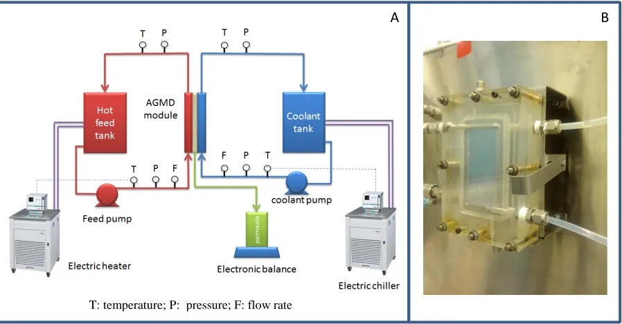
chiller and heater. A schematic diagram of the AGMD experimental unit is shown in Figure 6a.

Figure 6: a) Schematic of the AGMD experimental setup, b) Flat sheet AGMD module.

3.2.Experiment procedure

There are several features of the AGMD process that our mathematical model should be able

to predict, such as the feed and coolant outlet temperatures, mass flux, and outlet feed salinity.

However, not all of these features are important from a practical point of view and sometimes a

feature can be very difficult to measure experimentally. The mass flux of the AGMD is

considered as a very important feature should be measured with a high degree of accuracy

especially in a bench scale study. Therefore, our validation procedure was based on comparing

the predicted mass flux to the measured mass flux.

Reproducibility tests were initially conducted to determine the experimental error associated

with flux measurements. A sensitivity analysis using the mathematical model was conducted to

identify which operating parameters are likely to significantly affect the mass flux. A matrix of

experimental runs was then planned (Table 2) to map the operating conditions for the AGMD

process that would result in detectable variations in flux for the bench scale unit.

14

4. Result and discussion

4.1. Model validation at different operating parameters

The first set of experiments was conducted to test the reproducibility and to determine the

experimental errors. The measured water vapor flux at different feed water temperatures was

repeatable and the variation in flux was a maximum of +0.12 kg/m2·hr (2%).

The mathematical model results were then validated against different experimental data.

Figure 7 shows a comparison between the predicted mass fluxes and the measured water vapor

fluxes for a range of deionized feed water temperatures (40oC – 80oC). The model predicted an

exponential behavior of the AGMD flux as a function of feed water temperature. Such behavior

is not only supported by our experimental data but also reported in published AGMD literature

[14,17,37]. However, the validity of the mathematical model should not be judged based on

predicting the trend of the process but also on how closely it predicts the absolute experimental

data. Our current purpose of developing this model is to utilize it as a tool for further analyzing

the AGMD process and for scale-up. Such a goal may require relaxed a criterion toward which

we may judge the validity of our module. Nonetheless, the prediction of the model was within

the range of the experimental error.

Figure 7: Simulated and measured water vapor fluxes at different deionized feed water

temperatures (runs no. 11-15).

To validate the model further we replaced the deionized water (feed) with Red Sea water to

see how the model predicts the water vapor flux for a seawater salinity of 4.2 wt%. The distillate

conductivity was continuously measured to check for any pore wetting that may took place and

the distillate conductivity was always below 20 µS. As shown in Figure 8, the predicted water

vapor flux was also within the range of experimental error.

Figure 8: Predicted and measured water vapor fluxes at different seawater feed temperatures

15 The effect of air gap width was also investigated. As shown in Figure 9, the model predicted

a decay in flux as the air gap increased. This result agrees with the results reported by Kimra et

al. [18] and Jonsson et al. [20]. However, the model prediction for water vapor flux at different

air gap widths was not as good as were the predictions for variations in feed temperature.

Analysis of the results showed that the water vapor flux was very sensitive to the change of air

gap width, especially when it is very small. A reduction in air gap width results in higher

production capacity and higher errors. These errors are more significant when the air gap width

is very small. Therefore, any small error in measuring the gap width (i.e., by 0.1 mm) will affect

the water vapor flux significantly. The error of our measurements to the gap width was about +

0.5 mm. Our investigation showed that this was due to the deformation of the parafilm tape used

in sealing the module. Further experimental tests with a modified module are required in the

future to better evaluate the model prediction at small air gap width.

Figure 9: Predicted and measured water vapor fluxes as a function of air gap width (runs no

16-21).

Finally, the model was validated against experimental data using different membrane pore

sizes. The model prediction was good enough (±10%), although it didn’t predict well the data

(15%) at feed temperature of 70 ⁰C for the 0.45µm membrane (Figure 10). In this region the flux

is increasing significantly as feed temperature is increased, so variations in the inlet temperature

will have a larger effect on the measured flux compared to measurements at lower feed

temperatures, and the error of 15%appears reasonable.

Figure 10: Predicted and measured water vapor fluxes using different membrane pore sizes (runs

no 1-5 and 22-26).

4.2.AGMD process parameters analysis

The previous validation tests were reasonably sufficient to provide enough confidence in the

developed mathematical model. Therefore, the model was utilized for analyzing the complex and

interrelated AGMD process parameters that are considered essential for scaling-up the MD

16 judgments prior to making any decision. For example, the thermal efficiency, the temperature

gradient across and along the membrane, the flow rate, the membrane surface area, and the flow

regimes all have technical and economical dimensions. Some of these parameters are discussed

in the next section. The discussion will be based on the input data presented in Table 3 to the

mathematical model.

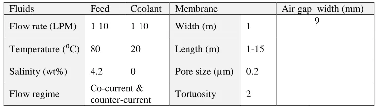
Table 3: The input parameters of the mathematical model used in analyzing AGMD process.

4.2.1.Effect of flow regime

The developed model can simulate both counter-current and co-current flow regimes for flat

sheet AGMD modules. Figure 11 and 12 show the temperature profile of the hot feed water and

the coolant temperatures inside the module. It might not be obvious which one would yield the

higher water vapor flux. The counter-current regime is characterized by constant temperature

difference along the module (this fact might not be true if the coolant flow rate is not equal to the

feed flow rate) while the co-current regime starts with a large temperature difference across the

membrane and decreases as the fluids move along the membrane. The effect of the flow regime

type on the water vapor flux will be discussed further in the next section.

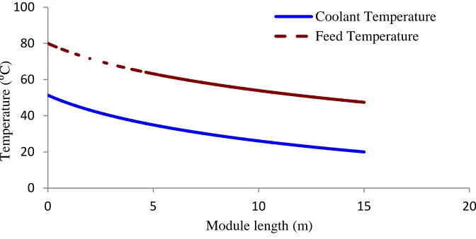
Figure 11: Simulating temperature profile along the membrane in counter-current flow regime.

Figure 12: Simulating temperature profile along the membrane in co-current flow regime.

4.2.2.Effect of membrane length

In a flat sheet module, whether a spiral wound or a plate and frame configuration, as the

membrane length increases the water vapor flux decreases (Figure 13). This behavior can be

explained by observing the change in the temperature difference across the membrane. As the

membrane length increases, enough time is provided for the fluids to exchange mass and heat

across the membrane. Therefore, the decrease in the hot feed water temperature and the increase

in the coolant temperature result in a decrease in the temperature difference across the membrane

(the driving force of mass transfer). Therefore, a gradual decrease in the flux takes place.

17 It is also observed that the decrease in the flux is faster in the co-current regime than in the

counter current one. The effect on the total permeate can be calculated by integrating the flux

along the membrane length. We found that, for a membrane length of 15 meters, the total

permeate in a co-current regime is less than that of the counter-current regime by about 5%. This

difference is expected to decrease as the membrane length decreases. However, in co-current

regime, heat recovery cannot be applied which makes the process thermally inefficient. Thus, in

the remaining discussion of this section, we will consider only the counter-current flow regime.

The effect of flow rate on water vapor flux is strongly linked to the membrane length. For a

fixed membrane length and equal feed and coolant flow rates, the driving force (temperature

difference across the membrane) increases as the feed and coolant flow rates were increased

together (Figure 14). At infinite flow rate, the maximum temperature difference across the

membrane that can be achieved is the difference between feed and coolant inlet temperatures: in our case, ∆Tmax = 60⁰C. As the flow rates decrease, there is more time for the fluids to exchange

heat inside the module, resulting in lowering the temperature difference across the membrane.

Therefore, depending on the residence time of the fluid inside the module the driving force will

change. If we assume that the cross sectional area of the fluid channel is constant along the

module which is usually the case, then we can relate the effect of flow rate and membrane length

(module length) to the residence time using the following equations:

𝑅𝑒𝑠𝑖𝑑𝑒𝑛𝑐𝑒𝑡𝑖𝑚𝑒= 𝑀𝑜𝑑𝑢𝑙𝑒_{𝐹𝑙𝑜𝑤}𝑣𝑜𝑙𝑢𝑚𝑒_{𝑟𝑎𝑡𝑒} = 𝐶𝑟𝑜𝑠𝑠_{𝑉𝑒𝑙𝑜𝑐𝑖𝑡𝑦∗𝐶𝑟𝑜𝑠𝑠}𝑠𝑒𝑐𝑡𝑖𝑜𝑛𝑎𝑙𝑎𝑟𝑒𝑎∗𝑀𝑜𝑑𝑢𝑙𝑒_{𝑠𝑒𝑐𝑡𝑖𝑜𝑛𝑎𝑙𝑎𝑟𝑒𝑎}𝑙𝑒𝑛𝑔𝑡ℎ (47)

From the equation above we observe that increasing the residence time of the module can be

achieved by either reducing the fluids flow velocity or increasing the membrane length.

However, in scaling-up the AGMD module we can only manipulate these two interlinked

parameters when they are within the module pressure drop limit. The increase in module

pressure drop caused by these parameters should not reach the liquid entry pressure (LEP) of the

membrane used. Thus, the increase in flux shown in Figure 14 and the experimental results

reported by Winter et al. [5] can be attributed mostly to the increase in the temperature difference

across the membrane and, to some extent, to the decrease in the temperature polarization effect.

Decoupling the effect of temperature polarization from the effect created by the change in

residence time through changing the fluid flow rate is quite challenging and might not give

18 fluid velocity, the module length should be increased according to Eq. (47). Such a change in

module length will change the process parameters in other aspects that lead to invalid

comparison.

Figure 14: Simulating the effect of the flow rate on the temperature difference across the

membrane (feed and coolant flow rates are maintained the same).

It is worth mentioning here that the majority of the laboratory-scale tests reported in the

literature are conducted with small membrane areas and at relatively high fluid velocity. These

conditions are considered to be favorable for high flux, especially when the ∆T between inlet temperatures of the fluids used in the test are relatively large (∆T=40-60 ⁰C). The flux at these

conditions will be large and far from the flux expected using large scale modules. For example, the 7-meter long membrane test conducted by Winter et al. [5] resulted in a ∆T of less than 10 _⁰C

even though the feed enters the module at 80⁰C and the coolant at 25⁰C. This small driving force

resulted in a water vapor flux that was slightly higher than 1 kg/m2.hr at feed flow rate of 200

L/hr. The performance of the membrane in an AGMD configuration is not expected to play a

major role at lower ∆T conditions, since the water vapor flux at these conditions is low and

within the range achievable by available commercial membranes. For instance, Figure 10 shows a slight increase in flux as the pore size increases from 0.2 µm to 0.45 µm at ∆T = 60 ⁰C across

the membrane. Additionally the thermal efficiency of AGMD is high because of the insulating

properties of the air gap, so changes in the thermal performance of membranes do not have a significant effect on the thermal efficiency of the MD process. But what is the optimal ∆T that an

MD module should operate at? The answer to this question will be discussed in the next section

where thermal efficiency and process economics are taken into consideration.

4.2.3.AGMD Process thermal efficiency

MD is a thermally driven process that utilizes phase change to achieve separation.

Conceptually, the thermal process is not an efficient technique for separation because the large

energy required to vaporize water is directed toward separating the major component (95% of

water) in the mixture [38]. The same concept is also applied in reverse osmosis where water is

19 In addition, the streams that leave the phase change separation process carry with them a

large quantity of heat and if this heat is not recovered (latent heat) the process becomes

inefficient. These main streams that leave the process are the brine and distillate.

An energy balance of the process shows that the maximum heat recovery is achieved when

the process brine and distillate temperatures approach the feed inlet temperature. This of course

requires exchanging the heat of the produced water vapor with the process feed and extending

the size of the separation unit to allow the brine to lose its heat through vaporization until its

temperature approaches the feed inlet temperature. In practice, the energy taken away by the

water vapor is recycled back to the process feed stream through a condenser to reduce the energy

input required to raise the feed temperature to the phase change temperature. Moreover, the

phase separation is conducted at a broad range of temperatures by extending the size of the unit

to reduce the energy loss through brine discharge. Both of these techniques are applied in the

conventional thermal desalination processes such as multi stage flash (MSF). However, the

increase of the unit size is limited by an increase in the capital cost of the unit. For example, the

size of a MSF unit is limited typically to 24 stages (with brine recirculation) and the brine

temperature exiting the unit is about 10-15 ⁰C higher than the process feed temperature [34,38].

This relatively high brine temperature is considered as the major heat loss in the MSF unit and

must be compensated by an external heat source to maintain continuity of the separation process.

AGMD is operated according to the same principle (Figure 15).

Figure 15: Typical design of AGMD.

In a once-through process like the AGMD shown in Figure 15, one can apply mass and

energy balance calculations on the feed stream to get the maximum achievable water recovery.

This recovery ratio is limited by the heated feed and the brine discharge temperatures according

to the following equations:

Mass balance:

20 where mF, mD and mB are the mass flow rates of the feed, distillate and brine streams,

respectively

Energy balance:

𝑚𝑓𝐶𝑝𝑇𝐹− 𝑚𝐷ℎ𝑔 − 𝑚𝐵𝐶𝑝𝑇𝐵 = 0 (49)

where TF and TB are the temperatures of the heated feed and brine discharge, respectively, hg is

the average latent heat of vapor, and Cp is the average specific heat of the feed.

From equation (48), we get:

𝑚𝐹𝐶𝑝𝑇𝐹− 𝑚𝐷ℎ𝑔−(𝑚𝐹− 𝑚𝐷)𝐶𝑝𝑇𝐵 = 0 (50)

Re-arranging the equation give:

𝑚𝐷

𝑚𝐹

=

(𝑇𝐹−𝑇𝐵) (ℎ𝑔_𝐶𝑝−𝑇𝐵)

(51)

In a process that has a heated feed entering at 80 ⁰C and a brine discharged at 30⁰C, the water

recovery is only 8.5%.

The heat input to this process can be calculated using the following equation:

𝐻𝑒𝑎𝑡𝑖𝑛𝑝𝑢𝑡= 𝑚𝐹𝑐𝑝(𝑇𝐹− 𝑇0) (52)

Where, To is the temperature of the feed after it leaves the heat recovery section. From equations

(51) and (52) we can calculate the specific heat requirement of the thermal process as:

𝑆𝑝𝑒𝑐𝑖𝑓𝑖𝑐ℎ𝑒𝑎𝑡𝑟𝑒𝑞𝑢𝑖𝑟𝑒𝑚𝑒𝑛𝑡 =𝐻𝑒𝑎𝑡_𝑚𝑖𝑛𝑝𝑢𝑡

𝐷

𝑆𝑝𝑒𝑐𝑖𝑓𝑖𝑐ℎ𝑒𝑎𝑡𝑟𝑒𝑞𝑢𝑖𝑟𝑒𝑚𝑒𝑛𝑡 = 𝑚𝐹𝑐𝑝(𝑇𝐹−𝑇𝑜) 𝑚𝐹(_{𝑇𝐹−𝑇𝐵})

(ℎ𝑔_{𝑐𝑝−𝑇𝐵})

(53)

After simplification,

𝑆𝑝𝑒𝑐𝑖𝑓𝑖𝑐ℎ𝑒𝑎𝑡𝑟𝑒𝑞𝑢𝑖𝑟𝑒𝑚𝑒𝑛𝑡 = 𝑇𝐹−𝑇𝑜

𝑇𝐹−𝑇𝐵(ℎ𝑔− 𝑐𝑝𝑇𝐵) (54)

(TF -T0) represents the driving force across the AGMD membrane and (TF – TB) represents

21 ∆Tdrop increases. As discussed earlier, decreasing the driving force temperature (∆Tcross) can be

achieved by increasing the residence time of the fluid inside the module through either extending

the module length or lowering the fluids flow rates. Increasing ∆Tdrop can be mainly achieved by

increasing the heated feed temperature or lowering the brine discharge temperature. Even though

the AGMD process can be operated at high temperature similar to MSF using steam, we are

going to assume that only low grade waste heat or solar energy is available. Therefore, we can

fix the TF to 80 ⁰C. In this way, our mathematical model can show how an increase in module

length or reducing feed flow rate would reduce ∆Tcross which in turn reduces the specific heat

requirement of the AGMD process (Figure 16).

Figure 16: Simulating the change in heat required and water vapor flux as a function of residence

time.

From the cost point of view, the saving in thermal energy consumption does not come free

and appears as an additional investment cost associated with increased membrane surface area. This brings us to the question of what is the optimal ∆Tcross that one should operate the AGMD

module at. A preliminary assessment can be made by considering the operational cost of the heat

input to the process and the capital cost of MD membrane. In undertaking this analysis the

following assumptions have been made:

- Energy cost: $0.05 per kwh (typical energy cost in the Middle East)

- Membrane cost: 36 $/m2 [39] (different membrane prices were reported in the literature

ranging from 10 to 100 $/m2 [40,41] and since this technology is not yet implemented at

large scale it is very difficult to predict a more accurate price of the membrane. However,

we chose the price in [39] because it falls in the range reported by Camacho et al. [40] for

membrane processes.

- Membrane life time: 5 years (typical membrane life in water industry)

Using the above costing figures along with our modeling prediction results, the graph in

Figure 17 shows an optimal point where the total energy consumption and membrane costs are at

the minimum. This value is expected to shift to less ∆Tcross as the cost of the membrane becomes

22 Figure 17: Simulated simple cost analysis of AGMD membrane and its energy use cost.

While this cost analysis provides some insight into economical tradeoffs between increased

thermal efficiency and capital cost, a more detailed life cycle analysis would provide a better

understanding of the cost issues associated with implementation of AGMD.

5. Conclusions

A co-current and counter-current flow 1-D mathematical model for a flat sheet module was

developed from the fundamental equations of mass and heat transfer. The model calculations

were based on dividing the AGMD module into different longitudinal zones. Normal to these

zones the module was sliced into small cells. The governing mass and energy equations were

applied to these slices and solved by iterative procedures. The model was then validated against

several experimental tests at different conditions such as different feed water temperatures, feed

salinity, membrane pore sizes, and air gap widths. The model predictionerror was within + 10%.

The model was utilized in analyzing some of the complex and interrelated AGMD process

parameters that are considered essential for scaling-up the process. The analysis showed that

fluid residence time inside AGMD module is very important for scaling-up the process since it

has direct effect on process flux and its thermal efficiency. The flux decreases as the membrane

length increases while it increases as flow rate increases. Furthermore, the total water vapor flux

in a co-current regime is always less than that of the counter-current regime. Additionally, the

thermal efficiency of the process increases as the membrane surface area increases which causes

the AGMD process to operate at low temperature difference across the membrane, leading to

lower water vapor flux.

Nomenclature

b Membrane thickness (m)

C Membrane mass transfer coefficient (kg/m2·hr·Pa)

c Molar concentration (kmole/m3)

cp Water specific heat (kJ/kg⁰C)

cphb Water specific heat at the bulk temperature of the hot feed channel (kJ/kg⁰C)

23 DAB Diffusion coefficient of water vapor in air (m2/s)

df Filament diameter (m)

dh Hydraulic diameter in a spacer filled channel (m)

g acceleration due to gravity (m/s2)

Hc Water film heat transfer coefficient of the coolant channel (kJ/m2·hr⁰C)

Hh Water film heat transfer coefficient of the hot feed channel (kJ/m2·hr⁰C)

hg Enthalpy of water vapor (kJ/kg)

hs Spacer thickness (m)

i Slice index

Jmv Water vapor flux by molecular diffusion (kg/m2·hr)

Jkv Knudsen mass flux of water vapor (kg/m2·hr)

Jv Water vapor flux (kg/m2·hr)

k average membrane thermal conductivity (W/m⁰C)

kair air thermal conductivity (W/m⁰C)

kf falling film thermal conductivity (W/m⁰C)

km membrane polymer thermal conductivity (W/m⁰C)

kl liquid water thermal conductivity (W/m⁰C)

kw cooling plate thermal conductivity (W/m⁰C)

Ks Spacer factor

L Membrane module length (m)

c

m Mass flow rate of the coolant (kg/hr)

h

m Mass flow rate of the hot feed (kg/hr)

mF Mass flow rate of the heated feed in once-through AGMD process (kg/hr)

mB Mass flow rate of brine discharge in once-through AGMD process (kg/hr)

mD Mass flow rate of the distillate in once-through AGMD process (kg/hr)

Mv Molecular weight of water vapor (Kg/kmole)

Nu Nusselt’s Number

P Total pressure of AGMD module (Pa)

P’f Water vapor partial pressure at the air gap and water falling film interface (Pa)

24 P’hm Water vapor partial pressure at the membrane and hot feed interface (Pa)

Pv Water vapor partial pressure (Pa)

Pr Prandtl’s Number

Q Heat flux (kJ/m2·hr)

Qc Heat flux in the cold feed channel (kJ/m2·hr)

Qh Heat flux in the hot feed channel (kJ/m2·hr)

Re Reynold’s number

R Universal gas constant

Tavg Average temperature inside the membrane (⁰C)

TB Temperature of the brine discharge in a once-through AGMD process (⁰C)

Tcb Bulk temperature of the coolant (⁰C)

Tcw Temperature of the cooling wall surface in the coolant channel (⁰C)

Tf Temperature of the falling film at the interface between the film and the air (⁰C)

TF Temperature of the heated feed in a once-through AGMD process (⁰C)

Tfw Film temperature in contact with the cooling wall (⁰C)

Thb Bulk temperature of the hot feed (⁰C)

Thm Temperature at the interface of hot feed and the membrane (⁰C)

Tma Temperature at the surface of the membrane facing the air channel (⁰C)

To Temperature of the feed after it leaves the heat recovery section in a once-through

AGMD process (⁰C)

Uc Overall heat transfer coefficient of the coolant channel (kJ/m2hr⁰C)

Uh Overall heat transfer coefficient of the feed channel (kJ/m2·hr·⁰C)

V Average velocity of water (m/hr)

Vfilament Volume occupied by the filament (m3)

Vtotal Total volume of the spacer (m3)

W width of the flat sheet module

x Length of AGMD module (m)

y Mole fraction of water vapor

yf Mole fraction of water vapor at the interface of the falling film

25

Greek symbols

δa Width of the air gap (m)

δc Thickness of the coolant wall (m)

δm Thickness of the membrane (m)

δf Thickness of the falling film (m)

ε Membrane porosity εs Spacer porosity

θ Angle between filaments (⁰) ρ Water density (kg/m3)

ρav Average liquid density (kg/m3)

ρl Liquid water density (kg/m3)

τ Membrane pores tortuosity µ Water dynamic viscosity (Pa·s)

References

[1] H. Maab, L. Francis, A. Al-Saadi, C. Aubry, N. Ghaffour, G.L. Amy and S.P. Nunes,

Synthesis and fabrication of hydrophobic polyazole membranes for seawater desalination,

Journal of Membrane Science 423-424 (2012) 11-19.

[2] Y.D. Kim, K. Thu, N. Ghaffour, K.C. Ng, A long-term performance investigation of

solar-assisted hollow fiber DCMD desalination system, Journal of Membrane Science 427

(2013) 345-364.

[3] E. Curcio, E. Drioli, Membrane distillation and related operations - A review, Separation

and Purification Reviews 34 (2005) 35-86.

[4] A.A. Hussain, J.M. Matar, R. Dores, C. Maltesh, S. Adham, Sustainable water production

by membrane distillation using low grade waste heat, World Congress/Perth Convention

and Exhibition Centre (PCEC), Perth, Western Australia September 4-9, 2011, Ref.

26 [5] D. Winter, J. Koschikowski, M. Wieghaus, Desalination using membrane distillation:

Experimental studies on full scale spiral wound modules, Journal of Membrane Science

375 (2011) 104-112.

[6] A. Kullab, Desalination using membrane distillation: Experimental and numerical study,

Doctoral Thesis 2011, Royal Institute of Technology, SE-100 44 Stockholm.

[7] J.H. Hanemaaijera, J.V. Medevoorta, A.E. Jansena, C. Dotremontb, E.V. Sonsbeekb, T.

Yuanc, L. De Ryckb, Memstill membrane distillation – a future desalination technology,

Desalination 199 (2006) 175–176.

[8] Z. Kui, W. Heinzl, F. Bollen, G. Lange, G. Van Gendt, A. Fane, Demonstrating

solar-driven membrane distillation using Memsys vacuum-multi-effect-membrane-distillation,

World Congress/Perth Convention and Exhibition Centre (PCEC), Perth, Western Australia

September 4-9, 2011 Ref.: IDAWC/PER11-214.

[9] R.B. Saffarini, E.K. Summers, H.A. Arafat,Technical evaluation of stand-alone solar

powered membrane distillation systems, Desalination 286 (2012) 332-341.

[10] N. Ghaffour, The challenge of capacity building strategies and perspectives for desalination

for sustainable water use in MENA, Desalination & Water Treatment 5 (2009) 48-53.

[11] C. Bier, U. Plantikow, Solar-Powered Desalination by Membrane Distillation (MD), IDA

World Congress on Desalination and Water Sciences, Abu Dhabi, November 18-24, 1995.

[12] A. Cipollina, M.G. Di Sparti, A. Tamburini, G. Micale, Development of a Membrane

Distillation module for solar energy seawater desalination, Chemical Engineering Research

and Design 90 (2012) 2101–2121.

[13] H. Chang, C.L. Chang , C.D. Ho, C.C. Li, Wang, P.H., Experimental and simulation study

of an air gap membrane distillation module with solar absorption function for desalination,

Desalination and Water Treatment 25 (2011) 251-258.

[14] M.A. Izquierdo-Gil, M.C. Garcia-Payo, C. Fernandez-Pineda, Air gap membrane

distillation of sucrose aqueous solutions, Journal of Membrane Science 155 (1999)

291-307.

[15] F.A. Banat, J. Simandl, Desalination by membrane distillation: A parametric study,

Separation Science and Technology 33(1998) 201-226.

[16] G.L. Liu, C. Zhu, C.S. Cheung, C.W. Leung,Theoretical and experimental studies on air

27 [17] F.A. Banat, J. Simandl, Therotical and experimental study in membrane distillation,

Desalination 95 (1994) 39-52.

[18] S. Kimura, S.I. Nakao, S.I. Shimatani, Transport phenomena in membrane distillation,

Journal of Membrane Science 33 (1987) 285-298.

[19] C. Gostoli, G.C. Sarti, S. Matulli, Low-Temperature Distillation through Hydrophobic

Membranes, Separation Science and Technology 22 (1987) 855-872.

[20] A.S. Jonsson, R. Wimmerstedt, A.C. Harrysson, Membrane distillation - a theoritical study

of evaporation through microporous membranes, Desalination 56(1985) 237-249.

[21] A.M. Alklaibi, N. Lior, Transport analysis of air-gap membrane distillation, Journal of

Membrane Science 255(2005) 239-253.

[22] R. Chouikh, S. Bouguecha, M. Dhahbi, Modelling of a modified air gap distillation

membrane for the desalination of seawater, Desalination 181 (2005) 257-265.

[23] M.N. Chernyshov, G.W. Meindersma, A.B. de Haan, Modelling temperature and salt

concentration distribution in membrane distillation feed channel, Desalination 157 (2003)

315-324.

[24] S. Bouguecha, R. Chouikh, M. Dhahbi, Numerical study of the coupled heat and mass

transfer in membrane distillation, Desalination 152 (2003) 245-252.

[25] J. Zhang, J.-D. Li, S. Gray, M. Duke, N. Dow, Modelling for scale-up of membrane

distillation processes, AWA Membranes and Desalination Specialty Conference III. 11-13

February, 2009, Sydney, NSW, paper 041.

[26] J. Zhang, J.-D. Li, S. Gray, Effect of applied pressure on PTFE membrane in DCMD,

Journal of Membrane Science, 369 (2011) 514-525.

[27] J. Zhang, J.-D. Li, S. Gray, Researching and modeling the dependence of MD flux on

membrane dimension for scale-up purpose, Desalination and Water Treatment 31 (2011)

144-150.

[28] J.H. Zhang, S. Gray, J.D. Li, Modelling heat and mass transfers in DCMD using

compressible membranes, Journal of Membrane Science 387 (2012) 7-16.

[29] C.M. Guijt, G.W. Meindersma, T. Reith, A.B., De Haan, Air gap membrane distillation - 1.

Modelling and mass transport properties for hollow fibre membranes, Separation and

28 [30] A.R. Dacosta, A.G. Fane, D.E. Wiley, Spacer Characterization and Pressure-Drop

Modeling in Spacer-Filled Channels for Ultrafiltration, Journal of Membrane Science 87

(1994) 79-98.

[31] A.F. Mills, Mass transfer 2001: Prentice Hall.

[32] R.B. Bird, W.E. Stewart, E.N. Lightfoot, Transport phenomena2006: Wiley.

[33] H.D. Baehr, K. Stephan, Heat and mass transfer. 3rd rev. ed2011, Berlin ; New York:

Springer. xxiv, 737 p.

[34] H.T. El-Dessouky, H.M. Ettouney, Fundamentals of Salt Water Desalination 2002:

Elseivier.

[35] M.H. Sharqawy, J.H.L. V, S.M. Zubair, Thermophysical properties of seawater: A review

of existing correlations and data, Desalination and Water Treatment 16 (2010) 354-380.

[36] L. Francis, H. Maab, A. AlSaadi, S. Nunes, N. Ghaffour, G.L. Amy, Fabrication of

Electrospun Nanofibrous Membranes for Membrane Distillation Application, Desalination

& Water Treatment 51 (2013) 1337–1343.

[37] M.C. Garcia-Payo, M.A. Izquierdo-Gil, C. Fernandez-Pineda, Air gap membrane

distillation of aqueous alcohol solutions, Journal of Membrane Science, 169 (2000) 61-80.

[38] N. Ghaffour, T.M. Missimer, G.L. Amy, Technical review and evaluation of the economics

of water desalination: Current and future challenges for better water supply sustainability,

Desalination 309 (2013) 197-207.

[39] C. Liu, A. Martin, Applying membrane distillation in high purity water production for

semiconductor industry, www.xzero.se, viewed July 2006.1.

[40] L.M. Camacho, L. Dumee, J. Zhang, J-D. Li, M. Duke, J. Gomez, S. Gray, Advances in

Membrane Distillation for Water Desalination and Purification Applications, Water 5

(2013) 94-196.

[41] Y. Lu, J. Chen, Optimal Design of Multistage Membrane Distillation Systems for Water

29 Table 1: Correlation equations of seawater physical properties.

No Property Correlation Reference

1 Water specific heat at constant pressure in kJ/kg.°C

T = Temperature in °C Validity range: 10 <T < 180°C S = salinity in g/kg Validity range: 20 < S < 160

Cp = (A + BT + CT2 + DT3) x10-3 A = 4206.8 - 6.6197 S + 1.2288x10-2 S2 B = -1.1262 + 5.4178x10-2 S - 2.2719x10-4 S2 C =1.2026x10-2 - 5.3566x10-4S + 1.8906x10-6S2 D = 6.8777xl0-7 +1.517x10-6 S - 4.4268x10-9 S2

[34]

2 Water dynamic viscosity in kg/m.s

T=Temperature in °C Validity range: 20 <T < 180°C S = salinity in g/kg Validity range: 0 < S < 130

𝜇=𝜇𝑤𝜇𝑅𝑥10−3

ln(𝜇𝑤) =−3.79418 +_{139.18 +}604.129_𝑇

𝜇𝑅= 1 +𝐴𝑆+𝐵𝑆2

𝐴= 1.474𝑥10−3_{+ 1.5𝑥10}−6_{𝑇 −3.927𝑥10}−8_𝑇2

𝐵= 1.0734𝑥10−5_−8.5𝑥10−8_{𝑇+ 2.23𝑥10}−10_𝑇2

[34]

3 Water thermal conductivity in watt/m.°C

T = Temperature in °C Validity range: 20 <T < 180°C S = Salinity in g/kg Validity range: 0 < S < 160

𝐿𝑜𝑔10(𝑘) =𝐿𝑜𝑔10(240 +𝐴𝑆) + 0.434 (2.3− 343.5+𝐵𝑆

𝑇+273.15)(1− 𝑇+273.15 647.3+𝐶𝑆)

1 3 A=2x10-4 B=3.7x10-2 C=3x10-2 [34]

4 Enthalpy of saturated water vapor in kJ/kg

T = Temperature in °C Validity range: 0.01-200 °C

H = 2501.689845 + 1.806916015 T + 5.087717x10-4 T2 - 1.1221x10-5T3

[34]

5 Latent heat of water evaporation in kJ/kg T = Temperature in °C Validity range: 5-200 °C

λ = 2501.897149 - 2.407064037 T + 1.192217x10-3 T2

- 1.5863x10-5 T3 [34]

6

Pure water partial pressure in bar

T = Temperature in K Validity range: 0 < T < 200°C

ln�_𝑃𝑃𝑑

𝑐𝑟𝑖𝑡�=

𝑇𝑐𝑟𝑖𝑡

𝑇 � 𝑏𝑖(1− 𝑇 𝑇𝑐𝑟𝑖𝑡)

(𝑖+1) 2 8

𝑖=1 Pcrit=220.93, Tcrit=647.25 K

b1=−7.8889166, b2=2.5514255, b3=−6.7161690,

b4=33.239495, b5=−105.38479, b6=174.35319,

b7=−148.39348, b8 = 48.631602

[5]

7 Correction for the seawater salinity effect on water vapor pressure

S = salinity in g/kg

Validity range: 0 < S < 130

𝑃𝑣

𝑃𝑣,𝑠𝑤= 1 + .57357(

𝑆

1000− 𝑆)

30 Table 2: Detailed conditions of the bench scale tests used in validating the model.

Run

No. Variable parameter Constant parameters

1-10

Temperature (40-80⁰C) (reproducibility test)

Hot feed: Red Sea water Hot feed flow rate: 1.5 LPM Coolant fluid: Deionized water Coolant inlet temperature: 20⁰C Coolant flow rate: 1.5 LPM Flow regime: Co-current Air gap width: 9 mm Pore size: 0.2 µm

11-15 Temperature

(40-80⁰C)

Hot feed: Deionized water Hot feed flow rate: 1.5 LPM Coolant fluid: Deionized water Coolant inlet temperature: 20⁰C Coolant flow rate: 1.5 LPM Flow regime: Co-current Air gap width: 9 mm Pore size: 0.2 µm

16-21 Air gap width (5,9,

and13mm)

Hot feed: Red Sea water Hot feed flow rate: 1.5 LPM Hot feed inlet temperature: 60,70⁰C Coolant fluid: Deionized water Coolant inlet temperature: 20⁰C Coolant flow rate: 1.5 LPM Flow regime: Co-current Pore size: 0.2 µm

22-26 Pore size (0.45μm)

31 Table 3: The input parameters of the mathematical model used in analyzing AGMD process.

Fluids Feed Coolant Membrane Air gap width (mm)

Flow rate (LPM) 1-10 1-10 Width (m) 1 9

Temperature (⁰C) 80 20 Length (m) 1-15

Salinity (wt%) 4.2 0 Pore size (µm) 0.2

Flow regime Co-current &

33 Figure 2: Magnification of two consecutive slices along an AGMD module.

Slice i

Slice i+1

Hot fluid channel

Hot fluid thin film

Membrane Air gap

Cold fluid

Cold fluid thin film

Cooling plate

Film condensate

mcicpiTci

mi-1_c pi-1Ti-1 i 1 i 1

∆QcidxiW =mcbcpi(Tcbi-Tcbi-1)

mi-1cpi-1Ti-1

UcidxiW(Tfi-Tcbi)

Slice i-1

mhicpiThi i _Si

∆Qhi=(mhbicpiThbi–

mhbi-1cpiThbi-1)/C

i i i Jv=C

∆P

∆Q i_=(h gJvi+

36 Figure 5:Scanning electron microscopy (SEM) of the active layer (left), support layer (middle)

and contact angle measurement of the commercial membranes.

Figure 6: a) Schematic of the AGMD experimental setup, b) Flat sheet AGMD module.

T: temperature; P: pressure; F: flow rate

37

Feed inlet temperature (oC)

30 40 50 60 70 80 90

W

at

er

v

apor

f

lux

(k

g

/m

2.h

r)

0 1 2 3 4 5 6 7

Simulated flux measured flux

Figure 7: Simulated and measured water vapor fluxes at different deionized feed water

temperatures (runs no. 11-15).

Feed inlet temperature (oC)

30 40 50 60 70 80 90

W

at

er

v

apor

f

lux

(k

g

/m

2 .h

r)

0 1 2 3 4 5 6 7

simulated flux kg/m2

.hr measured flux kg/m2.hr

38

Air gap width (mm)

4 6 8 10 12 14

W

at

er

v

apor

f

lux

(

k

g

/m

2 .h

r)

1 2 3 4 5 6 7

simulated flux at 60 o_C

measured flux at 60 o_C

measured flux at 70 o_C

simulated flux at 70 o_C

Figure 9: Predicted and measured water vapor fluxes as a function of air gap width (runs no

16-21).

Feed inlet Temperature (oC)

30 40 50 60 70 80 90

W

at

er

v

apor

f

lux

(

k

g

/m

2 .h

r)

0 1 2 3 4 5 6

7 _{measured flux for 0.45 mm pore size membrane}

measured flux for 0.2 mm pore size membrane predicted flux for 0.2 mm pore size membrane predicted flux for 0.45 mm pore size membrane

Figure 10: Predicted and measured water vapor fluxes using different membrane pore sizes (runs

39 Figure 11: Simulating temperature profile along the membrane in counter-current flow regime.

Figure 12: Simulating temperature profile along the membrane in co-current flow regime.

0 20 40 60 80 100

0 5 10 15 20

T

em

p

er

at

u

re (

⁰

C)

Module length (m)

Coolant Temperature Feed Temperature

0 10 20 30 40 50 60 70 80 90

0 2 4 6 8 10 12 14 16

T

em

p

er

at

u

re (

⁰

C)

Module length (m)

Coolant Temperature

40

Membrane length (m)

0 2 4 6 8 10 12 14 16

W at er v apor f lux ( k g /m 2 .h r) 1 2 3 4 5 6 co-current counter-current

Figure 13: Simulating the effect of membrane length on water vapor flux.

Flow rate (kg/hr)

0 100 200 300 400 500 600 700

∆ T ac ros s m em br ane ( o C ) 10 15 20 25 30 35 40 W at er v apor f lux ( k g /m 2 .h r) 0.5 1.0 1.5 2.0 2.5 3.0 3.5 ∆T

Water vapor Flux