A Generalized Technique in Numerical Integration

A Generalized Technique in Numerical Integration

HassanSafouhi1,

1_{Mathematical Division, Campus Saint-Jean}

University of Alberta

8406, 91 Street, Edmonton, Alberta T6C 4G9, Canada

Abstract.Integration by parts is one of the most popular techniques in the analysis of integrals and is one of the simplest methods to generate asymptotic expansions of integral representations. The product of the technique is usually a divergent series formed from evaluating boundary terms; however, sometimes the remaining integral is also evaluated. Due to the successive differentiation and anti-differentiation required to form the series or the remaining integral, the technique is difficult to apply to problems more compli-cated than the simplest. In this contribution, we explore a generalized and formalized integration by parts to create equivalent representations to some challenging integrals. As a demonstrative archetype, we examine Bessel integrals, Fresnel integrals and Airy functions.

1 Introduction

It is well known that in applied mathematics and in the numerical treatment of scientific problems, slowly convergent integrals occur abundantly. They are produced by approximation procedures de-pending on a parameter, iterative methods, quadrature schemes, perturbation techniques and reliable evaluation of functions defined by integrals. These slowly convergent integrals present severe nu-merical and computational difficulties. Traditional quadrature rules and summation techniques have failed to provide accurate approximations to such integrals. Numerous methods and techniques were developed for improving convergence of these challenging integrals [1–18] and extremely efficient methods were introduced such as numerical steepest descent, Filon-type and Levin-type methods. Unfortunately, their application to complicated integrals is extremely challenging. Examples of such integrals are the twisted tail, Bessel integrals, Sommerfeld integrals and the so-called molecular multi-center integrals involved in molecular structure calculations.

The technique of integration by parts has frequently been used to create divergent asymptotic se-ries representations of integrals. As an example, we consider the Euler sese-ries arising from integrating the Euler integral by parts:

_∞

x e−t

t dt∼ e−x

x

∞

l=0

(−1)ll!

xl, x→ ∞. (1)

In this example, the remaining integral afternintegrations by parts:

(−1)n_n! ∞ x

e−t

tn+1dt, (2)

is often discarded and the divergent series has either been summed straightforwardly or summed through the use of sequence transformations.

Another example of the use of integration by parts in numerical integration arises in [19], applied to the oscillatory spherical Bessel integral function involved in molecular integrals. Through a refor-malized integration by parts with respect toxdx, we transformed the initial spherical Bessel integral into an integral involving the simple sine function:

_∞

0 x

nxkˆν

_R 2γ(s,x)

_γ(s,x)nγ jλ(vx) dx =

_∞

0   d

xdx λ

xnx+λ−1kˆνR2γ(s,x) _γ(s,x)nγ



sin(x) dx. (3)

From a numerical point of view, the transformed sine integral function is more favorable than the initial Bessel integral function. The above integral transformation, which we caled theS transfor-mation, was successfully applied to all molecular integrals leading to an unprecedented accuracy and efficiency [19, 20]. However, this transformation requires the boundary terms to vanish at both limits of integration and was only applied to spherical Bessel integrals [21]. In the present work, we gen-eralize this approach to a larger class of integrals. This generalization does not require the boundary terms to vanish at both limits of integration. The contribution that will be introduced is a reformalized integration by parts with respect tow(x) dxfor some weight functionw(x) = xµ forµ ∈ Cwhose choice depends on the integrand. For the successive differentiation d

xµ_dx

k

fork=0,1,2, . . .required by this generalization, we will apply the Slevinsky-Safouhi formulae (SSF) [22].

We applied successfully the general reformalization of integration by parts to three well known challenging integrals, namely Bessel integrals, Fresnel integrals and Airy functions. The integral representations obtained for these integrals have better convergence properties and more favourable asymptotic behaviours.

For the computation of the integral representations, we propose a robust algorithm which will be referred to as the staircase algorithm. The algorithm uses both the boundary terms and the trans-formed integrals and progressively descends the integrand to an asymptotically favourable situation by applying the reformalized integration by parts at each iteration.

2 Slevinsky-Safouhi formulae (SSF) for differentiation

For more details on SSF and their applications, we refer the reader to [22, 23]. Applications of SSF in numerical integration of challenging integrals are presented in [24, 25].

Theorem 2.1 (The SSF 1 [22]) Let G(x)∈ Ck_{with the term}

d

xm_dx k

(x−n_{G(x))well-defined and easy}

to compute for m,n∈C. Forµ, ν∈C, the term

_d

xµ_dx k

(x−ν_{G(x))is given by:}

_d

xµ_dx k

(x−ν_G(x))=

k

i=0

Ai

kxn−ν+i(m+1)−k(µ+1)

_d

xm_dx i

In this example, the remaining integral afternintegrations by parts:

(−1)n_n! ∞ x

e−t

tn+1dt, (2)

is often discarded and the divergent series has either been summed straightforwardly or summed through the use of sequence transformations.

Another example of the use of integration by parts in numerical integration arises in [19], applied to the oscillatory spherical Bessel integral function involved in molecular integrals. Through a refor-malized integration by parts with respect toxdx, we transformed the initial spherical Bessel integral into an integral involving the simple sine function:

_∞

0 x

nxkˆν

_R 2γ(s,x)

_γ(s,x)nγ jλ(vx) dx =

_∞

0   d

xdx λ

xnx+λ−1 kˆνR2γ(s,x) _γ(s,x)nγ



sin(x) dx. (3)

From a numerical point of view, the transformed sine integral function is more favorable than the initial Bessel integral function. The above integral transformation, which we caled theS transfor-mation, was successfully applied to all molecular integrals leading to an unprecedented accuracy and efficiency [19, 20]. However, this transformation requires the boundary terms to vanish at both limits of integration and was only applied to spherical Bessel integrals [21]. In the present work, we gen-eralize this approach to a larger class of integrals. This generalization does not require the boundary terms to vanish at both limits of integration. The contribution that will be introduced is a reformalized integration by parts with respect tow(x) dxfor some weight functionw(x) = xµforµ ∈ Cwhose choice depends on the integrand. For the successive differentiation d

xµ_dx

k

fork=0,1,2, . . .required by this generalization, we will apply the Slevinsky-Safouhi formulae (SSF) [22].

We applied successfully the general reformalization of integration by parts to three well known challenging integrals, namely Bessel integrals, Fresnel integrals and Airy functions. The integral representations obtained for these integrals have better convergence properties and more favourable asymptotic behaviours.

For the computation of the integral representations, we propose a robust algorithm which will be referred to as the staircase algorithm. The algorithm uses both the boundary terms and the trans-formed integrals and progressively descends the integrand to an asymptotically favourable situation by applying the reformalized integration by parts at each iteration.

2 Slevinsky-Safouhi formulae (SSF) for differentiation

For more details on SSF and their applications, we refer the reader to [22, 23]. Applications of SSF in numerical integration of challenging integrals are presented in [24, 25].

Theorem 2.1 (The SSF 1 [22]) Let G(x)∈ Ck_{with the term}

d

xm_dx k

(x−n_{G(x))well-defined and easy}

to compute for m,n∈C. Forµ, ν∈C, the term

_d

xµ_dx k

(x−ν_{G(x))is given by:}

_d

xµ_dx k

(x−ν_G(x))=

k

i=0

Ai

kxn−ν+i(m+1)−k(µ+1)

_d

xm_dx i

(x−n_{G(x)), (4)}

with coefficients:

Ai k=

  

1 for i=k

(n−ν₋(k−1)(µ+1))A0_k−1 for i=0, k>0 (n−ν+i(m+1)−(k−1)(µ+1))Ai_k−1+A_ki−1₋₁ for 0<i<k.

(5)

Moreover, for m−1, these coefficients have the explicit expression:

Ai k=

i

j=0

(−1)i−j_{(n−ν+j(m+1)−(k−1)(µ+1))} k,µ+1

(m+1)ij! (i− j)! , (6)

where(x)n,kis the Pochhammer k-symbol [26] and can be computed as n−1

l=0

(x+kl).

The SSF 2 corresponds to the case (µ, ν,m,n)=(0,0,1,0) which is the most popular.

3 Reformalized integration by parts

Definition 3.1 Let the following operator be known as integration of a function f(x)byw(x)dx, for some weight functionw(x):

f(x)w(x)dx. (7)

Let us begin with the general integral f(x)dxfor which the general antiderivative isF(x). By performing the substitution(x)↔ x, we arrive at f((x))d(x). The differential element d(x) can be written as(x)dxand by denotingw(x)=(x), we assert that this becomesintegration by w(x)dx, with a weight functionw(x).

The integral f(x)dx generally does not have a simple antiderivative; however, the integral

f((x))(x)dxmost certainly has an antiderivative with a simple representation with respect to

the first integral, notablyF((x)).

Integration by parts is one of the main methods used in the formation of asymptotic series expan-sions of a given integral. When integrating by parts, we generally begin with:

g(x)d

dxh(x)=

d

dx(g(x)h(x))−h(x)

d

dxg(x). (8)

When integrating by parts byxdxas in [19], we begin with:

g(x) d

xdxh(x)=

d

xdx(g(x)h(x))−h(x)

d

xdxg(x). (9)

Our method, which formalizes this process is suitable for integrals of composite functions, like the aforementioned f((x)).

In order to expand integrals of composite functions in asymptotic series, we must incorporate this formalism with integration by parts byw(x) withw(x)=xµforµ∈Z. Naturally, then, we begin with:

g(x) d

xµ_dxh(x)= d

xµ_dx(g(x)h(x))−h(x) d

By using the weight functionw(x)=xµ, we must continue by integrating byxµdx. To clarify the following process, we make use of these functionals ofg(x) andh(x):

Gl(x)=(−1)l

_d

xµ_dx l

g(x) and Hl(x)=

_d

xµ_dx −l

h(x). (11)

The computation of the functionalsGl(x) is obtained using SSF. With these functionals, we can rewrite (10) as:

G0(x)H0(x)= _xµd_dx(G0(x)H1(x))+G1(x)H1(x), (12)

and therefore with integration byxµ_{dx, the first term on the right hand side becomes a boundary term} and the second term on the right hand side becomes the transformed integral.

Let f(x)∈ Cm_{[a,b] be integrable on [a,b] and be of the general form:}

f(x)=G0(x)H0(x)xµ, (13)

where the functionalsGl(x) andHl(x) are defined as in (11). Let us consider the integral:

b

a f(x)dx

= b

a G0(x)H0(x)x

µ_{dx. (14)}

By integrating the right hand side by parts, we obtain: b

a G0(x)H0(x)x

µ_dx=G

0(x)H1(x) b

a+ b

a G1(x)H1(x)x

µ_{dx. (15)}

And, by integrating by parts anothern−1 times, we obtain the equivalent representation: b

a f(x)dx

=

n−1

l=0

Gl(x)Hl+1(x) b

a+ b

a Gn(x)Hn(x)x

µ_{dx. (16)}

Naturally, then, the question arises in how to use the equivalent representations. Indeed, one could simply neglect the remaining integral asn → ∞ and form a series from boundary terms; or, one could evaluate the boundary terms up to mand continue to numerically evaluate the new integral. To these two proposed methods, there exist advantages and disadvantages. The boundary terms, for example, usually form divergent series, which are generally challenging to sum; however, that the integral becomes a simply series can lead to reduced calculation times. The new integral, on the other hand, may be asymptotically favourable; however, the computation of the new integrand may become challenging after a certain order.

The next algorithm we propose is actually a blend of the two extremes outlined above. We numer-ically integrate the integral to some pointx=x0,a<x0<b. At such a point, we now apply the first iteration of the reformalized integration by parts by xµ_{dxto the remaining integral. We continue by} evaluating the boundary terms atx=bandx= x₀and we numerically integrate the new integral to another pointx=x1,x₀ <x1<b. We continue in this manner until the desired accuracy is attained. This blended algorithm will be aptly known as the staircase algorithm, as it progressively descends the integrand into an evermore asymptotically favourable situation.

By using the weight functionw(x)=xµ, we must continue by integrating byxµdx. To clarify the following process, we make use of these functionals ofg(x) andh(x):

Gl(x)=(−1)l

_d

xµ_dx l

g(x) and Hl(x)=

_d

xµ_dx −l

h(x). (11)

The computation of the functionalsGl(x) is obtained using SSF. With these functionals, we can rewrite (10) as:

G0(x)H0(x)= _xµd_dx(G0(x)H1(x))+G1(x)H1(x), (12)

and therefore with integration byxµ_{dx, the first term on the right hand side becomes a boundary term} and the second term on the right hand side becomes the transformed integral.

Let f(x)∈ Cm_{[a,b] be integrable on [a,b] and be of the general form:}

f(x)=G0(x)H0(x)xµ, (13)

where the functionalsGl(x) andHl(x) are defined as in (11). Let us consider the integral:

b

a f(x)dx

= b

a G0(x)H0(x)x

µ_{dx. (14)}

By integrating the right hand side by parts, we obtain: b

a G0(x)H0(x)x

µ_dx=G

0(x)H1(x) b

a+ b

a G1(x)H1(x)x

µ_{dx. (15)}

And, by integrating by parts anothern−1 times, we obtain the equivalent representation: b

a f(x)dx

=

n−1

l=0

Gl(x)Hl+1(x) b

a+ b

a Gn(x)Hn(x)x

µ_{dx. (16)}

Naturally, then, the question arises in how to use the equivalent representations. Indeed, one could simply neglect the remaining integral asn → ∞ and form a series from boundary terms; or, one could evaluate the boundary terms up to mand continue to numerically evaluate the new integral. To these two proposed methods, there exist advantages and disadvantages. The boundary terms, for example, usually form divergent series, which are generally challenging to sum; however, that the integral becomes a simply series can lead to reduced calculation times. The new integral, on the other hand, may be asymptotically favourable; however, the computation of the new integrand may become challenging after a certain order.

The next algorithm we propose is actually a blend of the two extremes outlined above. We numer-ically integrate the integral to some pointx=x0,a<x0<b. At such a point, we now apply the first iteration of the reformalized integration by parts by xµ_{dxto the remaining integral. We continue by} evaluating the boundary terms at x=bandx= x₀ and we numerically integrate the new integral to another pointx=x1,x₀<x1<b. We continue in this manner until the desired accuracy is attained. This blended algorithm will be aptly known as the staircase algorithm, as it progressively descends the integrand into an evermore asymptotically favourable situation.

This methodology is concisely summarized in:

Algorithm 3.2 (The Staircase Algorithm) The approximations to the integral_ab f(x)dx take the following form. For a<x0<b, initialize:

S0= x0

a G0(x)H0(x)x

µ_{dx, (17)}

For l=1,2, . . . ,n,and for the sequence{xl}nl=1that satisfies a<xl−1<xl<b define:

Sl=Sl−1+Gl(x)Hl+1(x) b

xl−1 +

xl

xl−1

Gl(x)Hl(x)xµ_{dx, (18)}

and the approximations to the integral_abf(x)dx form the sequence{Sl}nl=0.

3.1 Bessel Integrals

The integral that follows appeared in Numerical Recipes as a computational challenge and an example of application of sequence transformations:

I1=

∞

0

x

x2₊₁J0(x) dx=

∞

0 1

x2₊₁J0(x)xdx. (19)

We begin by noting that the integrand f(x) satisfies f(x)∈ C∞_{(−∞,+∞). This integral is already} in an appropriate form for the reformalized integration by parts, since we can subdivide the integrand as the product of:

G0(x)= 1

x2₊₁, H0(x)=J0(x), and w(x)=x. (20) Starting with these root forms, we can explicitly develop the functionalsGl(x) andHl(x) as:

Gl(x)= 2

l_l!

(x2₊₁₎l+1 and Hl(x)=x

l_{Jl(x), (21)}

through Bessel function properties. The integral then has the equivalent representation:

I1=2nn!

∞

0

xn+1

(x2₊₁₎n+1 Jn(x) dx. (22)

In (22), all the boundary terms vanish.

In Numerical Recipes, the value of the integral is determined through Cauchy’s residue theorem to beI1=K0(1). Although the equivalent representation does not give this formula, it follows from (22) that:

2n_Γ(n+1) ∞

0

xn+1

(x2₊₁₎n+1 Jn(x) dx=K0(1). (23)

3.2 Fresnel Integrals

Let us consider the Fresnel-type integral:

I2(a, v)=

_∞

a sin(vx

2_{)dx. (24)}

We begin by noting that the integrand f(x) satisfies f(x) ∈ C∞_{(−∞,+∞). By identifying the} functions:

G0(x)=1

x, H0(x)=sin(vx2), and w(x)=x, (25)

the functionalsGl(x) andHl(x) can be readily determined as:

Gl(x)= (2l)!

2l_l!x2l+1 and Hl(x)=

sin(vx2−lπ/2)

(2v)l . (26)

It then follows straightforwardly that (24) has the equivalent representations:

I2(a, v)=₍₄(2_vn₎n)!_n!

_∞

a

sin(vx2_−nπ/2)

x2n dx− n−1

l=0

2 (2l)! (4v)l+1_l!

sin(vx2_{−(l+1)π/2)}

x2l+1

_x=a, (27)

through application of the reformalized integration by parts..

Similarly, we obtain the equivalent representation for ˜I2(a, v)=_a∞cos(vx2_{)dxwhich is given by:}

˜

I2(a, v)= (2n)! (4v)nn!

∞

a

cos(vx2_−nπ/2)

x2n dx− n−1

l=0

2 (2l)! (4v)l+1l!

cos(vx2_{−(l+1)π/2)}

x2l+1

_x=a. (28)

3.3 Airy Functions

The Airy functions are given by:

I3(a,z) =

∞

a cos _x3

3 +zx

dx

=

∞

a

cos(zx) cos

x3 3

−sin(zx) sin

x3 3

dx. (29)

We begin by noting that the integrand f(x) satisfies f(x) ∈ C∞_{(−∞,+∞). By identifying the} functions:

G0(x)=x−2 cos_{sin (}zx), H0(x)= cos_{sin x3}

3

, and w(x)=x, (30)

the functionalsGl(x) andHl(x) can be readily determined as:

Gl(x)=

−d

x2_dx l

x−2 cos

sin (zx) and Hl(x)= cossin _x3

3 −

lπ

2

. (31)

The integral then has the equivalent representation:

I3(a,z) =

n−1

l=0

(−1)l+1

x3l+2

l

i=0

Ai l(zx)icos

x3

3 +zx−

(l+1₋i)π

2

_a

+ (−1)n

∞

a n

i=0

Ai n(zx)i

x3n cos _x3

3 +zx−

(n−i)π

2

3.2 Fresnel Integrals

Let us consider the Fresnel-type integral:

I2(a, v)=

_∞

a sin(vx

2_{)dx. (24)}

We begin by noting that the integrand f(x) satisfies f(x) ∈ C∞_{(−∞,+∞). By identifying the} functions:

G0(x)=1

x, H0(x)=sin(vx2), and w(x)=x, (25)

the functionalsGl(x) andHl(x) can be readily determined as:

Gl(x)= (2l)!

2l_l!x2l+1 and Hl(x)=

sin(vx2−lπ/2)

(2v)l . (26)

It then follows straightforwardly that (24) has the equivalent representations:

I2(a, v)=₍₄(2_vn₎n)!_n!

_∞

a

sin(vx2_−nπ/2)

x2n dx− n−1

l=0

2 (2l)! (4v)l+1_l!

sin(vx2_{−(l+1)π/2)}

x2l+1

_x=a, (27)

through application of the reformalized integration by parts..

Similarly, we obtain the equivalent representation for ˜I2(a, v)=_a∞cos(vx2_{)dxwhich is given by:}

˜

I2(a, v)= (2n)! (4v)nn!

∞

a

cos(vx2_−nπ/2)

x2n dx− n−1

l=0

2 (2l)! (4v)l+1l!

cos(vx2_{−(l+1)π/2)}

x2l+1

_x=a. (28)

3.3 Airy Functions

The Airy functions are given by:

I3(a,z) =

∞

a cos _x3

3 +zx dx = ∞ a

cos(zx) cos

x3 3

−sin(zx) sin

x3 3

dx. (29)

We begin by noting that the integrand f(x) satisfies f(x) ∈ C∞_{(−∞,+∞). By identifying the} functions:

G0(x)=x−2 cos_{sin (}zx), H0(x)= cos_{sin x3}

3

, and w(x)=x, (30)

the functionalsGl(x) andHl(x) can be readily determined as:

Gl(x)=

−d

x2_dx l

x−2 cos

sin (zx) and Hl(x)= cossin _x3 3 − lπ 2 . (31)

The integral then has the equivalent representation:

I3(a,z) =

n−1

l=0

(−1)l+1

x3l+2

l

i=0

Ai l(zx)icos

x3

3 +zx−

(l+1₋i)π

2

_a

+ (−1)n

∞

a n

i=0

Ai n(zx)i

x3n cos _x3

3 +zx−

(n−i)π

2

dx. (32)

4 Numerical Results and Discussion

As previously alluded to, a numerical evaluation of the integrals I1, I2(a, v), ˜I2(a, v) andI3(a,z) can be achieved through a multiplicity of methods. Historically, the popular candidates were the summation of the generally divergent boundary terms, although the transformed integral has also been used in cases where the boundary terms vanished. In this work, we implemented the Staircase algorithm, as the newest method to evaluate these integrals and serves as an original contribution to the overall methodology we will be developing.

The selection of an appropriate sequence{xl}nl=0 for the integration subintervals in the Staircase

algorithm is critical. This sequence should leave the integral subintervals to be numerically integrable – the points cannot be spaced so far apart that a quadrature routine is incapable of providing the solution. Conversely, the sequence should not be so squished that the sum of the boundary terms and the integral subintervals introduces a reduction in accuracy from the addition of a very large number and a very large negative number. Generally speaking, the dependence onlof the sequence{xl}nl=0

resides in the integrand. For the cases at hand, the integrands are oscillatory, and thus if the difference

xl−xl−1is on the same order of magnitude as the difference between successive zeros of the integrand, both of the aforementioned scenarios can be averted.

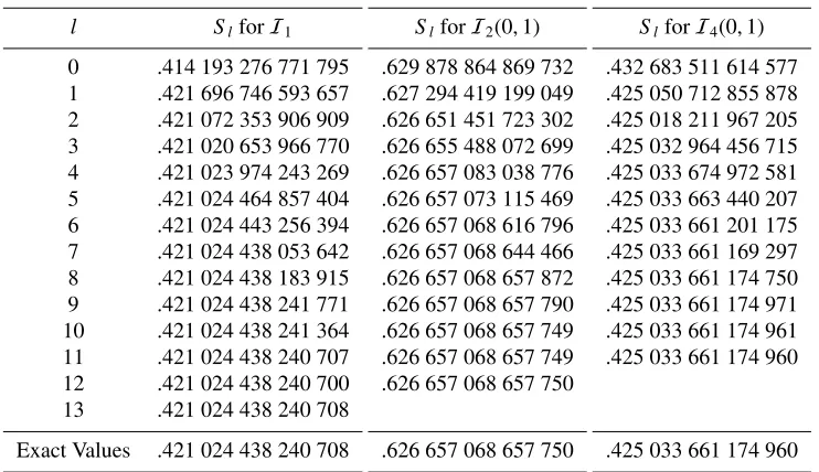
As can be seen from the numerical table, the algorithm is capable of reaching high accuracy. This is mainly due to the fact that reformalized integration by parts progressively descends the integrand to an asymptotically favourable situation.

5 Numerical tables

Table 1.Numerical Results of Staircase Algorithm applied to Bessel integralsI1withxl=2π(l+1), Fresnel integrals withI2(0,1).xl= √2π(l+1), and Airy functionsI4(0,1) withxl=√36π(l+1).

l SlforI1

0 .414 193 276 771 795 1 .421 696 746 593 657 2 .421 072 353 906 909 3 .421 020 653 966 770 4 .421 023 974 243 269 5 .421 024 464 857 404 6 .421 024 443 256 394 7 .421 024 438 053 642 8 .421 024 438 183 915 9 .421 024 438 241 771 10 .421 024 438 241 364 11 .421 024 438 240 707 12 .421 024 438 240 700 13 .421 024 438 240 708 Exact Values .421 024 438 240 708

SlforI2(0,1) .629 878 864 869 732 .627 294 419 199 049 .626 651 451 723 302 .626 655 488 072 699 .626 657 083 038 776 .626 657 073 115 469 .626 657 068 616 796 .626 657 068 644 466 .626 657 068 657 872 .626 657 068 657 790 .626 657 068 657 749 .626 657 068 657 749 .626 657 068 657 750

.626 657 068 657 750

SlforI4(0,1) .432 683 511 614 577 .425 050 712 855 878 .425 018 211 967 205 .425 032 964 456 715 .425 033 674 972 581 .425 033 663 440 207 .425 033 661 201 175 .425 033 661 169 297 .425 033 661 174 750 .425 033 661 174 971 .425 033 661 174 961 .425 033 661 174 960

Acknowledgement

The author acknowledges the financial support for this research by the Natural Sciences and Engi-neering Research Council of Canada (NSERC) – Grant RGPIN-2016-04317.

References

[1] C. Brezinski, M. Redivo-Zaglia,Extrapolation Methods: Theory and Practice(Edition North-Holland, Amsterdam, 1991)

[2] P. Rabinowitz, Numer. Algo.3, 17 (1992) [3] J. Lyness, ANZIAM J.42, 181 (2000)

[4] A. Sidi, Practical Extrapolation Methods: Theory and Applications(Cambridge U. P., Cam-bridge, 2003)

[5] J. McWilliams, J. Balusek, H. Gray, Comm. Stat. Simu. Comput.33, 1 (2004) [6] D. Levin, A. Sidi, Appl. Math. Comput.9, 175 (1981)

[7] H. Gray, S. Wang, SIAM J. Numer. Anal.29, 271 (1992) [8] R. Slevinsky, H. Safouhi, Numer. Algor.48, 301 (2008)

[9] R. Slevinsky, H. Safouhi, Int. J. Quantum Chem.109, 1741 (2009) [10] D. Huybrechs, S. Vandewalle, SIAM J. Numer. Anal.44, 1026 (2006) [11] D. Levin, J. Comput. Appl. Math.67, 95 (1996)

[12] S. Olver, IMA J. Num. Anal.26, 213 (2006)

[13] J. Lyness, J. Lottes, BIT Numer. Math.49, 397 (2009) [14] J. Lyness, G. Hines, Math. Comp.12, 24 (1986)

[15] K. Kim, R. Cools, L. Ixaru, Appl. Numer. Math.46, 59 (2003) [16] G. Evans, K. Chung, J. Webster, App. Numer. Math.34, 85 (2000) [17] G. Adam, A. Nobile, IMA J. Numer. Anal.11, 271 (1991)

[18] G. Adam, S. Adam, N.M. Plakida, Comput. Phys. Comm.154, 49 (2003) [19] L. Berlu, H. Safouhi, J. Phys. A: Math. Gen.36, 11791 (2003)

[20] L. Berlu, H. Safouhi, J. Phys. A: Math. Gen.37, 3393 (2004) [21] H. Safouhi, J. Math. Chem.29, 213 (2001)

[22] R. Slevinsky, H. Safouhi, J. Comput. App. Math.233, 405 (2009) [23] R. Slevinsky, H. Safouhi, Numerical Algorithm66, 457 (2014)

[24] P. Gaudreau, R. Slevinsky, H. Safouhi, SIAM J. Sci. Comput.34, B65 (2012) [25] R. Slevinsky, H. Safouhi, Numer. Algor.60, 315 (2012)