An investigation into the parallel implementation of JPEG for image compression

Parallel Implementation of

JPEG

for Image Compression

by

Paul Darbyshire

lie LIBRARY zjl

Thesis submitted for the degree of

Master of Engineering

in the Department of

FTS THESIS 621.367 DAR 30001005244209 Darbyshire, Paul

Paul Darbyshire

declare that this thesis entitled

A n Investigation into the Parallel Implementation of J P E G

for Image Compression

is m y o w n work and has not been submitted previously, in whole or

part in respect of any other academic award.

[%.!%.($ ^

This thesis has b e e n a long time in the m a k i n g , and during that time I h a v e h a d help from m a n y people, to w h o m I o w e m u c h . First, to m y original principal supervisor, A n n Pleasants, w h o b e c a m e m y second supervisor after a career m o v e to Fiji. T h a n k s to Ann's help a n d persistence over the years, a n d particularly in the last three m o n t h s via constant emails to and from Fiji, this thesis has finally b e e n assembled in a presentable form. I w o u l d also like to thank Ji D o n g W a n g w h o took over the role o f principal supervisor for a period o f about a year and s h o w e d m e h o w to write papers. I w o u l d also like to thank Elizabeth H a y w o o d w h o has b e e n m y principal supervisor for only a short while but w h o has helped greatly with content suggestions and editing. This thesis w o u l d not h a v e b e e n possible without them.

Finally, I h a v e saved this to last, but perhaps it should h a v e b e e n first. T o m y wife K a y and son A d a m , w h o h a v e both put u p with m e for the duration o f this thesis. W e h a v e missed m u c h together over the time that I h a v e spent o n this. T o A d a m , w h o always w a n t e d to d o something with m e , but w o u l d quietly shut the door and let d a d w o r k , thanks. T o K a y w h o w o u l d not complain w h e n w e missed doing things together so I could get this d o n e , thanks.

of J P E G for Image Compression

Abstract

This research develops a parallel algorithm to implement the J P E G standard for continuous tone still picture compression to be run on a group of transputers. T h e processor-farm paradigm is adopted. This research shows this to be the best paradigm for use with the J P E G baseline algorithm on the measured component times within the algorithm. T h e speedup of the parallel algorithm is investigated and measured against a single processor version. A n optimal distribution of J P E G components on the processors within the processor farm is established.

The research focuses on the investigation of the optimal number of processors, which can be used effectively for a J P E G implementation adopting the processor-farm paradigm. This optimal n u m b e r is termed the saturation point. O n c e the saturation point has been reached, it is s h o w n that the parallel algorithm's speedup cannot be improved without the redistribution of tasks in the farm, regardless of h o w m a n y extra processors are used. Further distributions of processing tasks are investigated with the aim of extending the saturation point. It is s h o w n that the saturation point can be extended, and the distributions of tasks to achieve this are demonstrated. It is also s h o w n that while the saturation point can be increased, the gains are minimal and m a y not be worth the cost of the extra processor. In fact, the algorithm speedup diminishes after the addition of the third processor, up to saturation point.

A simulation algorithm is devised using Java, which takes advantage of the multi-threaded nature of the language. A technique is developed for simulating the processor-farm paradigm. This technique uses the concept of the Java threadgroup as a basis for a simulated processor, and a Java thread allocated to that group, as a process belonging to this processor. A process scheduling scheme is refined which allows the simulated parallel system to be monitored over simulated scheduling rounds. A scheme is also s h o w n that simulates the message passing of the transputer.

CONTENTS

CHAPTER 1 INTRODUCTION 1

CHAPTER 2 A SURVEY OF IMAGE COMPRESSION TECHNIQUES 6

2.1 INTRODUCTION 6 2.2 IMAGE REPRESENTATION 7

2.3 ENTROPY 9 2.3.1 Measuring Entropy 10

2.4 ENTROPY CODERS 12 2.4.1 Huffman Coding 12

2.4.2 Arithmetic Coding 15

2.5 IMAGE COMPRESSION 17 2.5.1 Predictive Coding 18

2.5.2 Transform Coding 21

2.5.2.1 Fourier Transform 24 2.5.2.2 Discrete Cosine Transform 26

2.5.2.3 Karhunen-Loeve Transform 27 2.5.2.4 Walsh-Hadamard Transform 28

2.5.2.5 Summary 29 2.5.3 Vector Quantization 32

2.6 SELECTION OF INTERNATIONAL STANDARD 34 2.7 RECENT COMPRESSION TECHNIQUES 35

2.7.1 Wavelet Compression 55

2.7.2 Fractal Compression 39

2.7.3 Comparison with JPEG 43

3.1 INTRODUCTION 46

3.2 JPEG STANDARD 46

3.2.1 Lossless Vs. Lossy Compression 47

3.2.2 DCT-based Compression Overview 49

3.2.3 JPEG Steps 54

3.2.3.1 Level Shift 55 3.2.3.2 D C T 55 3.2.3.3 Quantization 57 3.2.3.4 Baseline Coder 58 3.2.4 Compressed Data Formats 62

3.3 PARALLEL SYSTEMS A N D PROCESSING 62 3.3.1 Supporting Architecture 65

3.3.1.1 M I M D vs. SIMD 65 3.3.1.2 Memory Organization 67 3.3.1.3 The Transputer 69 3.3.2 Parallel Processing Software Paradigms 72

3.3.2.1 Homogeneous Parallelization 73 3.3.2.2 Heterogeneous Parallelization 74 3.3.2.3 Processor Farm Paradigm 75

3.3.3 Performance 77

3.4 S U M M A R Y 82

CHAPTER 4 PARALLEL JPEG IMPLEMENTATION 83

4.1 INTRODUCTION 83

4.2 METHODOLOGY 84 4.3 PARALLEL PROCESSING ENVIRONMENT 85

4.4 SEQUENTIAL ALGORITHM 87 4.5 PARALLEL ALGORITHM 90 4.6 COMPONENT TIMING ISSUES A N D COMMUNICATION 96

4.6.1 Component Timing 96

4.6.1.1 Hardware Issues 96 4.6.1.2 Software Issues 98 4.6.1.3 Expected Time Savings of PV1 99

4.6.2 Communication Timing 100

4.6.2.1 Expected Time Savings of PV1 Recalculated 105 4.6.2.2 Impact of Communication Times on Optimal Placement 106

4.7 D E V E L O P M E N T O F A G E N E R A L P A R A L L E L A L G O R I T H M 108

4.7.2 Processor Farm Implementation 110

4.7.3 Development of Processor Farm Algorithm Ill

4.7.3.1 Saturation Point 114 4.7.3.2 Expected vs Measured times of P V 2 118

4.7.3.3 Impact of Saturation Point on Optimal Task Placement 121

4.8 C O N C L U S I O N 124

CHAPTER 5 PARALLEL JPEG SIMULATION USING JAVA 126

5.1 INTRODUCTION 126

5.2 IMPLEMENTATION OF TASKS AS JAVA THREADS 127

5.3 THREAD SCHEDULING IN JAVA 129 5.3.1 Thread states in Java 129

5.3.2 Scheduling in the Java VM 131

5.4 DEVELOPMENT OF PARALLEL JPEG SIMULATION ALGORITHM 133

5.4.1 Thread Groups 135

5.4.2 Construction of Simulation Objects 137

5.4.3 Simulation Algorithm 139

5.4.4 Processor Communication 142

5.5 JAVA SIMULATION PROBLEMS 144 5.5.1 Garbage Collector 144

5.5.2 Inappropriate Behaviour of Master Processor Send Thread. 145

5.5.3 Network Timing Considerations 146

5.5.4 Processor Speed When Running Simulation 149

5.6 SIMULATION RESULTS 151

5.7 CONCLUSIONS 159

CHAPTER 6 CONCLUSION 161

6.1 S U M M A R Y 161 6.2 CRITICAL APPRAISAL 162

6.3 FURTHER RESEARCH 164

BIBLIOGRAPHY 168

APPENDIX A IMAGES AND TABLES 177

A.2 I M A G E S 178 A.3 C H A P T E R 4 T A B L E S 179

A.4 JPEG P R O C E D U R E D I A G R A M S 182

A.5 SIMULATION R U N D A T A 186

APPENDIX B PARALLEL C TRANSPUTER CODE 190

B.l INTRODUCTION 190

B.2 CONFIGURATION FILE FOR SEQUENTIAL P R O G R A M SV1 191

B.3 P A R A L L E L C C O D E OF P R O G R A M SV1 192 B.4 CONFIGURATION FILE FOR PARALLEL P R O G R A M PV1 198

B.5 PARALLEL C C O D E OF P R O G R A M PV1 199

B.5.1 Code for Processor PQ 199

B.5.2 Code for Processor P] 204

B.6 CONFIGURATION FILE FOR PROCESSOR F A R M P R O G R A M PV2 206 B.7 P A R A L L E L C C O D E OF P R O C E S S O R F A R M P R O G R A M PV2 207

B.7.1 Code for Master task 207

B.7.2 Code for Worker task 212

B.8 INCLUDE FILES 214

APPENDIX C JAVA PARALLEL SIMULATION CODE 216

C l INTRODUCTION 216 C.2 I M A G E FILE H E A D E R CLASS 217

C.3 C O M P R E S S E D FILE H E A D E R CLASS 218

C.4 T O K E N OBJECT CLASS 219 C.5 W O R K E R T H R E A D OBJECT CLASS 220

FIGURE 2.1 CONSTRUCTION OF DIGITAL IMAGE 8

FIGURE 2.2 DEPICTION OF ENTROPY vs. REDUNDANCY IN A DATA SOURCE [90] 10

FIGURE 2.3 HUFFMAN TREE BUILT FROM FREQUENCIES IN TABLE 2.2 13 FIGURE 2.4 INITIAL INTERVAL DIVISIONS ACCORDING TO PROBABILITIES 15 FIGURE 2.5 SUBSEQUENT DIVISION OF PREVIOUS SYMBOL INTERVALS 16

FIGURE 2.6 PIXEL NEIGHBOURHOOD 18

FIGURE 2.7 DPCM LOSSY ENCODER BLOCK DIAGRAM 20

FIGURE 2.8 GENERAL STEPS IN TRANSFORM CODING 21 FIGURE 2.9 TYPICAL I/O CHARACTERISTICS OF A QUANTIZER [48] 22

FIGURE 2.10 ENERGY PACKING EFFICIENCY AS A FUNCTION OF CORRELATION COEFFICIENT [15] 30 FIGURE 2.11 ENERGY PACKING EFFICIENCY AS A FUNCTION OF TRANSFORM BLOCK SIZE [15] 30 FIGURE 2.12 DECORRELATION EFFICIENCY AS A FUNCTION OF THE CORRELATION COEFFICIENT [ 15]... 31

FIGURE 2.13 DECORRELATION EFFICIENCY AS A FUNCTION OF TRANSFORM BLOCK SIZE [15] 31

FIGURE 2.14 VECTOR QUANTIZATION BLOCK DIAGRAM 33 FIGURE 2.15 COMPARISON OF SINE W A V E AND DAUBECHIES WAVELET 36

FIGURE 2.16 SOME WELL K N O W N WAVELET FAMILIES 36 FIGURE 2.17 DISCRETE FOURIER BASIS FUNCTIONS VS. SCALED WAVELET BASIS FUNCTIONS 37

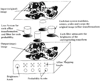
FIGURE 2.18 OUTLIERS A N D TRENDS COEFFICIENTS 38 FIGURE 2.19 FRACTAL GENERATED FERN LEAF 40 FIGURE 2.20 SIERPINSKY'S TRIANGLE CONSTRUCTION 40 FIGURE 2.21 BARNSLEY'S PHOTOCOPY MACHINE 41

FIGURE 3.1 STRUCTURE OF LOSSLESS ENCODER 47

FIGURE 3.2 PREDICTION OF PIXELZFROM 3 NEIGHBOURS 48 FIGURE 3.3 GENERAL STRUCTURE OF DCT BASED ENCODER 48

FIGURE 3.4 IMAGE BLOCKS 49 FIGURE 3.5 APPLICATION OF ONE-DIMENSIONAL DCT 50

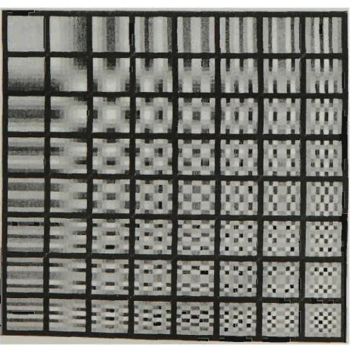
FIGURE 3.6 APPLICATION OF A TWO-DIMENSIONAL DCT 51 FIGURE 3.7 TRANSFORMED BLOCK COEFFICIENTS 52 FIGURE 3.8 TWO-DIMENSIONAL 8 x 8 DCT BASIS FUNCTIONS [70] 52

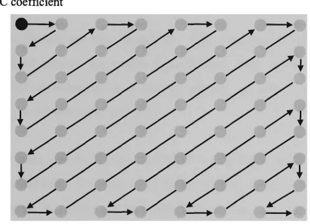
FIGURE3.9 ZIG-ZAG SEQUENCE FOR 8x8 BLOCK OF TRANSFORM COEFFICIENTS 53

FIGURE 3.10 AC COEFFICIENT PROBABILITY IN ZIG-ZAG INDEX [69] 54 FIGURE3.11 SIGNAL FLOW GRAPH FOR FAST DCT [14], [70] 56 FIGURE 3.12 BASELINE SEQUENTIAL-DCT ENCODER MODEL 59

FIGURE 3.16 S O M E SHARED M E M O R Y ARCHITECTURES 68 FIGURE 3.17 GENERALIZED DIAGRAM OF A TRANSPUTER 70 FIGURE 3.18 GENERAL FORM OF TRANSPUTER SYSTEM CONNECTED TO PC HOST 71

FIGURE 3.19 S O M E EXAMPLES OF TRANSPUTER TOPOLOGIES 71 FIGURE 3.20 HOMOGENEOUS PARALLELIZATION [10] 73 FIGURE 3.21 HETEROGENEOUS PARALLELIZATION [10] 74 FIGURE 3.22 PROCESSOR FARM METHODOLOGY 76 FIGURE 3.23 AMDAHL'S L A W vs. GUSTAFSON-BARSIS L A W 79

FIGURE 3.24 SPEEDUP CURVE FOR MANDELBROT DATA FROM TABLE 3.6 80 FIGURE 3.25 SIMPLIFIED REPRESENTATION OF H.261 ENCODING EXECUTION 80 FIGURE 3.26 IDEALIZED vs. ACTUAL PERFORMANCE FOR THE H.261 ENCODER [92] 81

FIGURE 4.1 PHYSICAL TRANSPUTER CONFIGURATION WITH THREE PROCESSORS 86

FIGURE4.2 SEQUENTIAL ALGORITHM SV1 MAIN COMPONENTS 87 FIGURE 4.3 AVERAGE PROCESSING TIMES PER IMAGE BLOCK 90 FIGURE 4.4 TOTAL PROCESSING TIMES PER PROCESSOR 91 FIGURE 4.5 STRUCTURE OF PARALLEL ALGORITHM PV1 94 FIGURE 4.6 COMPARATIVE CHART REPRESENTATION OF TABLE 4.5 97

FIGURE 4.7 COMPARISON OF COMMUNICATION TIMING BETWEEN DIFFERENT PROCESSORS 101

FIGURE 4.8 INTER-PROCESSOR COMMUNICATION MODELS 102 FIGURE 4.9 S U M OF PROCESSING TIMES WITH COMMUNICATION ALLOWANCE 104

FIGURE 4.10 PIPELINE IMPLEMENTATION OF SVI WITH 3 PROCESSORS 109 FIGURE 4.11 CALCULATED PROCESSING TIMES OF PROCESSORS IN PIPELINE 109 FIGURE 4.12 APPLICATION OF PROCESSOR FARM TECHNIQUE TO IMAGE COMPRESSION 110

FIGURE 4.13 STRUCTURE OF PARALLEL ALGORITHM PV2 114 FIGURE 4.14 COMPARISON OF OVERALL PROCESSING TIMES OF P0 VS P, 116

FIGURE4.15 EXPECTED IDLE TIME O N P0 117

FIGURE 4.16 ASSUMED CONFIGURATION OF PROCESSOR FARM 121 FIGURE 4.17 COMPARISON OF SATURATION POINTS WITH DIFFERENT TASK CONFIGURATIONS 122

FIGURE 4.18 PROGRESSIVE ALGORITHM TIME SAVINGS VS NUMBER OF PROCESSORS 123

FIGURE 5.1 JAVA THREAD STRUCTURE 128

FIGURE 5.2 JAVA THREAD STATES 130 FIGURE 5.3 JAVA THREAD SCHEDULING HIERARCHY 132

FIGURE 5.4 ABSTRACT VIEW OF A MULTI-PROCESSOR SYSTEM 134

FIGURE 5.8 STRUCTURE OF OBJECTS IN JAVA SIMULATION 139

FIGURE 5.9 PSEUDOCODE FOR SIMULATION ALGORITHM SJM2 142

FIGURE 5.10 U S E OF JAVA VECTORS TO SIMULATE MESSAGE PASSING 143 FIGURE 5.11 DELAY TIMES TO SIMULATE NETWORK COMMUNICATION DELAYS 148

FIGURE 5.12 ASSUMED SIMULATION NETWORK TOPOLOGY 148 FIGURE 5.13 COMPARATIVE CHART REPRESENTATION OF TABLE 5.1 150

FIGURE 5.14 COMPARATIVE LINE CHART REPRESENTATION OF TABLE 5.2 153 FIGURE 5.15 COMPARATIVE LINE CHART REPRESENTATION OF TABLE 5.3 156 FIGURE 5.16 COMPARATIVE LINE CHART REPRESENTATION OF TABLE 5.4 156 FIGURE 5.17 COMPARISON LINE CHARTS OF TRENDS IN INPUT QUEUE LENGTH 157

FIGURE 6.1 POSSIBLE USE OF MULTIPLE PROCESSOR FARMS 165

FIGURE A.l GENERATION OF TABLE OF HUFFMAN CODE SIZES 182

FIGURE A.2 GENERATION OF TABLE OF HUFFMAN CODES 183 FIGURE A.3 SEQUENTIAL ENCODING OF AC COEFFICIENTS WITH HUFFMAN CODING 184

List of Tables

TABLE 2.1 8-BIT GREY SCALE VALUES FOR BLOCK IN FIGURE 2.1 8

TABLE 2.2 SOURCE SYMBOL FREQUENCY DISTRIBUTION 13 TABLE 2.3 SOURCE SYMBOLS A N D PROBABILITIES 15 TABLE 2.4 COMPARISON OF COMPRESSION METHODOLOGIES 44

TABLE 2.5 COMPARISON OF ARTIFACT BEHAVIOUR OF METHODOLOGIES 44

TABLE 3.1 LUMINANCE QUANTIZATION TABLE 58

TABLE 3.2 LIST OF LUMINANCE CODE LENGTHS FORHUFFMAN TABLES 60 TABLE 3.3 SET OF LUMINANCE CODE VALUES FOR CORRESPONDING CODE LENGTHS IN TABLE 3.2 60

TABLE 3.4 AMPLITUDE CATEGORIES FOR COEFFICIENTS 61 TABLE 3.5 FLYNN'S PARALLEL SYSTEMS CLASSIFICATION SCHEME 65

TABLE 3.6 EXECUTION TIMES FOR DISPLAYING MANDELBROT SET 79

TABLE4.1 OVERALL TIMING FOR ALGORITHM SV1 89

TABLE 4.2 TIME TRIAL AVERAGES FOR SV1 COMPONENTS 89

TABLE 4.3 PROCESSING TASK SYMBOLS 93 TABLE 4.4 OVERALL TIMING RESULTS FOR PV1 95 TABLE 4.5 COMPARISON TIMING DATA PER BLOCK OF N O N I/O PROCESSES O N ALL PROCESSORS 97

TABLE 4.6 RATIOS OF COMPONENT PROCESSING TIMES OF PI I PO 99 TABLE 4.7 COMMUNICATION TIMING SUMMARY BETWEEN PO A N D P ; ,P2 101

TABLE 4.8 PROCESSOR INVOLVEMENT IN COMMUNICATION 103

TABLE 4.9 OVERALL TIMING RESULTS FOR PV2 120

TABLE 5.1 COMPARISON OF TRANSPUTER AND PENTIUM PROCESSOR TIMES 150

TABLE 5.2 OVERALL AVERAGES OF THE FIRST 100 TIME QUANTUMS 152 TABLE 5.3 AVERAGES OF FIRST 100 TIME QUANTUMS UP TO zsnd DEATH 155 TABLE 5.4 AVERAGES OF FIRST 100 TIME QUANTUMS AFTER rsnd DEATH 155

TABLE A.l TIMING DATA FOR ALGORITHM SV1 COMPONENTS 179

TABLE A.6 TRANSMISSION & RECEIPT TIMES OF 4096 BLOCKS (4/8 BYTES/ELEMENT) 181

TABLE A.7 TIMING TRIALS FOR JPEG COMPRESSION COMPONENTS 186

CHAPTER 1

INTRODUCTION

The use of digital images dates back to the early 1920s w h e n digitized pictures of world n e w s events were first transmitted by submarine cable between N e w York and London [28]. It w a s not until the m i d to late 1960s that the use of digital images became m o r e wide spread. Then the computing power, speed and storage capacity in third generation computers were such that practical applications involving the use of digital images became feasible, for example, the storage and transmission of satellite images.

It soon became apparent that in dealing with images, computer systems would have to cope with huge amounts of data. Image compression w a s recognized as an important

problem. For example, a small image of 640 x 480 pixels using 8 bit V G A colour m o d e requires about 2.4 x IO6 bits. If 24-bit true colour is used then the image requires three times that amount. Digital images from Landsat satellites are taken using multispectral scanners in four spectral bands, and s o m e images are in excess of 300 megabytes. It is not only professionals in these specialist fields that are affected by image size. T h e average Internet user today is well aware of the time it takes to download the large graphics embedded in w e b pages.

operation loses s o m e information that is not detectable by the h u m a n eye thus allowing far higher compressions. It is based on the Discrete Cosine Transform ( D C T ) . B y using the D C T , the image is first transformed into its frequency domain resulting in less correlated coefficients that m a k e the quantization and coding more effective. J P E G has almost b e c o m e a household word, with users of the internet familiar with the term due to the 'jpg' format images available o n the web. M o s t image manipulation software tools also support the J P E G format, which has b e c o m e a format of choice for people providing large images via the Internet.

The DCT is a computationally intensive task requiring a reasonable amount of computing power in order to code images in an acceptable time. For this reason, m a n y implementations of J P E G are realized through hardware solutions, or J P E G chips, to achieve higher speed. However, as m o r e demands are placed for faster implementations for real time applications, traditional serial processors have begun to encounter physical limitations which inhibit further speed increases [40]. For example, no signal can travel faster than the speed of light, which indicates an upper limit to the speed at which algorithms can be processed. T o overcome this, components are being m a d e smaller which limits the distance that signals are transmitted during processing, but then heat dissipation becomes a problem.

One strategy used to overcome these limits is parallel processing. In a parallel system, multiple processors are connected and the processing is distributed to the processors so the various tasks can be executed simultaneously. T h e aim of parallel processing is that if a problem takes T time units to process on a single processor system, then on an TV processor system it will take T/N time units. This theoretical speedup is of course never reached due to practical considerations like communication delays between processors, and the overhead associated with the overall management of the network of processors. However, considerable speed advantages can be gained by application of a parallel programming paradigm to a suitable problem.

as any possible algorithmic parallelization. With the transform coding approach of J P E G , the image is broken into fixed sized sub-sections called blocks, and these are processed independently of each other. It is this independent processing of the blocks that suggest a possible data parallel approach. A n algorithm parallelization is also possible, as J P E G involves a number of distinct steps that must be applied to each block.

The purpose of this research is to investigate the application of parallel programming techniques to the J P E G international standard using a suitable parallel programming

paradigm. This research initially uses a transputer based network of processors for the hardware platform. A single processor algorithm, implementing the J P E G baseline sequential m o d e is constructed for use as a benchmark. A simple parallel version using two processors is then developed for initial testing, and finally a general parallel algorithm implementing the processor-farm paradigm is constructed.

Run time data is then gathered, and an optimal placement of processor tasks is shown for the network of processors. F r o m the data obtainable, an extrapolation of speedup

calculations indicated unexpected results, and from this, a hypothesis w a s formed that indicated a limit to the number of processors that could be effectively used b y the processor-farm paradigm implementing J P E G . This limit on the number of processors is called the saturation point. This number w a s initially calculated at 7 processors. Further, a hypothesis is m a d e that indicates this number m a y be extended by redistribution of tasks a m o n g the processors once the initial saturation point has been reached.

In order to test these hypotheses a simulation algorithm is constructed which runs on a Pentium 2 0 0 M H z processor. T h e simulation algorithm is implemented using Java

This simulation allows the behaviour of the processor-farm paradigm to be observed w h e n m o r e processors are added, regardless of the number of physical processors available. T h e simulation is then used to obtain further results on the parallel J P E G implementation to test the hypothesis. The results collected support the original hypothesis concerning the saturation point and the estimate for its number at 7 processors. Further, it is s h o w n with data collected from the simulation, that once reached, the saturation point can be extended by redistribution of the tasks a m o n g the processors. Optimal configurations for this extension are shown.

The Java simulation is platform independent due to the nature of Java, and thus capable of running on any platform which provides a Java Virtual Machine ( V M ) . This results in another outcome of this research, being an algorithm, which is suitable for a distributed system.

A number of papers resulted from this research. These are:

• "Parallel Implementation of the JPEG Still Picture Compression Algorithm", Darbyshire, Pleasants and W a n g [21], presented at the Australian Pattern Recognition Society Student Conference in 1996.

• "Using Java to Simulate Multi-processor Systems", Darbyshire P [20], in print with Department of Information Systems working paper series, Victoria University of Technology.

• "Implementation of a Parallel Image Compression Algorithm Using Java", Darbyshire and W a n g [22], presented at the 1997 D I C T A conference at Massey University, Auckland as a Technical Keynote Presentation.

Chapter 3 provides an in depth look at the J P E G standard, and covers the operation of the baseline sequential m o d e of operation. T h e D C T technique, which is at the heart of the J P E G algorithms, is discussed and a fast version of this is presented. T h e J P E G algorithms highlighted in this chapter are used in the construction of the research parallel algorithms. This chapter also investigates the development of parallel architectures, and the parallel paradigms c o m m o n l y used to build software for multi-processor systems. T h e selection of a suitable paradigm for application to J P E G is discussed.

In Chapter 4, a parallel implementation of JPEG is constructed in two different stages, and data collected from trial runs of these algorithms are compared with those of a

J P E G algorithm constructed for a single processor system. Using the data obtained, the parallel system overhead is investigated and the results used to develop an optimal placement of tasks on processors, which maximizes parallelism. The concept of a limit to the number of processors that can be effectively used is investigated.

In Chapter 5, a simulation program that implements the JPEG parallel algorithm of Chapter 4 is constructed in the J A V A programming language. This simulation program exploits the multi-threaded nature of J A V A and allows the behaviour of the parallel algorithm constructed in Chapter 4 to be investigated with a varying number of processors. B y using J A V A , this simulation is platform independent and can be run on any system providing a J A V A V M . The concept of the processor limit developed in Chapter 4 is further investigated using this simulation program.

The final chapter presents the conclusions of the research carried out in Chapters 4 and 5 and discusses associated aspects. A critical appraisal of the research in this

CHAPTER 2

A SURVEY OF IMAGE COMPRESSION TECHNIQUES

2.1 Introduction

Image compression is needed to both reduce the storage requirements of an image and the transmission time in telecommunication applications. T h e goal of research into

image compression techniques is to produce schemes that give high compression ratios, run efficiently, and result in a high quality reconstructed image. Image compression can be regarded as a particular instance of general data compression except that it takes advantage of characteristics unique to images and the w a y our visual system views them. All compression aims to minimize the number of information carrying units in the signal that represents the image [48].

There are two phases to compression, and these are the encoding and decoding processes. In s o m e circumstances the reconstructed data must be identical with the original, for example, in textual documents distortion is unacceptable, and in medical images where patient safety is of paramount importance. W h e n a perfect reconstruction of an image is required, compression is constrained by the entropy of the image. T o increase image compression, techniques were developed that rely on s o m e degradation to the image that is not detectable to the h u m a n eye.

In order to achieve better compression ratios for images, different techniques are used to exploit various image properties. Predictive coders are supported by a statistical

loss. Adding quantization to this process increases compression at the expense of s o m e loss of information and hence image quality. Transform coding first m a p s the image into a domain where it becomes far m o r e amenable to compression, before quantization and entropy coding. Transform coding allows m o r e compression to take place before serious image degradation. Vector quantization is another effective image coding technique.

To enable the transmission and exchange of images in telecommunication

applications, there w a s a requirement for s o m e standard for the storage and compression of photographic images. This w a s the driving force behind the development of the J P E G1 International Standard. Research has not waned since the acceptance of this standard, and since then other techniques proposing higher compression while retaining image quality have attracted interest. T h e most notable are Wavelet and Fractal Image compression.

This chapter outlines the main areas of image compression. It starts by discussing the theoretical basis to compression. It gives an overview of the main image compression

techniques, but concentrates on those that form part of the J P E G standard. T w o of the more recent techniques are discussed and then compared to J P E G .

2.2 Image Representation

It is useful to first describe how images are represented digitally. The representation will depend on whether the image is greyscale or colour. This thesis is concerned

only with greyscale images, hence only these are described here.

A digital image is a computer representation of a continuous tone still picture. The digital image is obtained b y analog to digital conversion, which is analogous to

samples are then represented as numerical values for digital storage. In a greyscale image such as Figure 2.1, each sample value represents a luminance figure from a

scale that normally ranges from 0-255, with 8-bit samples. Each sample's luminance value is set independent of its neighbours.

Figure 2.1 Construction of digital image

T h e sampling process naturally loses information, but if the samples along each scan line are close enough, a reasonable representation of a continuous tone image is obtained. A sampling rate that will obtain good quality images is 400 dots per inch (dpi). Each image sample is called a,pixel (or pel), short for picture element. In the 8-bit digital image s h o w n in Figure 2.1, the white outlined square represents a block of 8x8 pixels, w h o s e pixel values are shown in Table 2.1. A value of zero is used for

black, and 255 for white. All other values are varying shades of grey.

Table 2.1 8-bit grey scale values for block in Figure 2.1 162 168 171 178 182 194 193 199 162 168 171 177 178 191 189 196 163 168 170 176 177 188 189 194 164 168 170 175 177 186 189 192 164 168 170 175 177 186 187 189 164 168 170 175 178 185 184 186 165 169 172 176 178 184 185 185 166 169 174 176 178 183 186 186

2.3 Entropy

Compression techniques exploit redundancy in the data source. Redundancy was explored in detail in a landmark paper by C.E. Shannon [78], while at Bell2 Laboratories. In this paper, Shannon investigates the transmission of information over a communication channel, and the coding process the transmitter uses to change the information into a form suitable for transmission.

Shannon investigated the difference between the information rate and the data rate of a data source. In a digital system, the bit rate is the product of the sampling rate and

the n u m b e r of bits in each sample, and is usually constant. However, Shannon observed the difference between the bit rate and the information rate of a real signal. This difference is the redundancy of the data source. Shannon used the term entropy to describe the information content of a data source.

Messages from most data sources have a degree of redundancy built into them. W h e r e an information source produces messages by selectively selecting symbols from a discrete alphabet, the probabilities of choosing s o m e symbols are dependent on previous choices. For example, in the English language words beginning with the letter q are followed by the letter u, so the placement of the letter u is governed by the statistics of the information source, not by any freedom of choice within the message. Statistically speaking the letter u is redundant and need not be stored or transmitted.

One way to measure the redundancy of a signal is to exploit the statistical predictability of the signal. T h e information content or entropy of a data source is a function of h o w different it is from the predicted value. According to Shannon's theory, any signal that is completely predictable carries no information [90]. For example, a sine w a v e is highly predictable because it is periodic. At the opposite extreme, noise is completely unpredictable.

Entropy is a term borrowed from thermodynamics, and then used as a measure of information in a random signal by Hartley [37]. Entropy is a quantification of the

information content of the symbols in a message from a given data source. With the entropy quantified, the redundancy rate is then k n o w n and a coding algorithm can be devised to remove this redundancy. The relationship between entropy and redundancy in a source is depicted in Figure 2.2. If the signal level and frequency of a transmission are used to denote an area, this sets a limit on the information capacity. A s in Figure 2.2, most real signals occupy only a part of that area. The entropy is the actual area occupied by the signal, and is the area that must be transmitted [90].

Signal level

Frequency

Figure 2.2 Depiction of entropy vs. redundancy in a data source [90]

2.3.1 Measuring Entropy

To calculate the entropy of a source we need to calculate the probabilities of the occurrence of the elements of the source [79], If an arbitrary element s\ of source S, occurs with probability pt, then the information content I, contained within that occurrence is:

I(st) = -logPi bits. (2.1)

When the base of the logarithm in (2.1) is 2 then I(s>) is expressed in bits. It is the m i n i m u m number of bits with which this symbol can be represented. T h e information

per symbol I(SJ) averaged for all elements over the whole alphabet of S, is the entropy H(S) of the source. Then

M M

H(S) = 2p,I(3i) = -YxPt^iPi ^

1=1 /=i

where M is the number of elements in S. In an image, the entropy is defined in terms of the probability of occurrences of the various pixel values. The entropy defined in

(2.2) is the first-order entropy of the source. It takes into account only the relative probabilities of the M possible input values, and no consideration is given to the fact that a particular input m a y have statistical dependence on previous inputs [28] [48] [33]. If successive inputs are independent, then the first-order entropy Hj(S) from (2.2) forms a lower bound on the average number of bits per input required to code a sequence of inputs from S [28].

If successive inputs of S are dependent, then higher-order entropies that give a better lower bound for a source can be calculated as:

M M

H2(S) = - £ £ p(wtxWj)log2 pfwt.wj) (2.3)

t=i j=i

In (2.3), H2(S) represents the second-order entropy of S and the function p(wit wj) is the joint probability density function of the two random variables wt and Wj. Third

and higher order entropies can be similarly defined if the inputs have a statistical dependence on the previous two or more inputs. These higher order entropies Hn(S) then become the lower bound on the number of bits required to code the sequence. It can be shown [28], that H. (S) > H2 (S) > ... > Hn (S).

Higher order entropies are usually not pursued, as the cost in computation to obtain them is prohibitive. However, for 6-bit raw image data it has been estimated [75] that

the first, second and third-order entropies are approximately 4.4, 1.9 and 1.5 bits per pixel respectively.

According to Shannon's noiseless coding theorem [78] [79], a source can be losslessly encoded to an average bit rate arbitrarily close to but not less than the entropy of the

m u c h redundancy is removed. That is, by h o w close to the entropy of the source the coders can get. The m a x i m u m achievable lossless compression C, is defined by:

average bit rate of original raw data n entropy of the source data H(S)

2.4 Entropy Coders

The coding process removes some redundancy from the data stream by storing the symbols in fewer bits than is used in the original source. The decoding process reverses the coding by adding the redundancy back in, resulting in the restoration of the original data stream. Coders that lose no information during this process are termed lossless, while those that do are k n o w n as lossy coders.

Entropy coders aim to remove the maximum redundancy while remaining lossless. They aim to operate at the entropy bit-rate level and thus achieve near to the theoretical m a x i m u m compression in (2.4). Thus, the entropy of a source forms the dividing line between lossy and lossless coders. The best k n o w n entropy coders are the Huffman coder and the arithmetic coder. Both of these coders are used by the J P E G standard.

2.4.1 H u f f m a n Coding

Huffman coding was devised by D.A.Huffman in 1952 [42]. Huffman compression takes advantage of the statistics of the data source by assigning variable length codes to elements of this data source. If all elements of a source were equally probable then fixed-length block coding would be an optimal strategy. In practice, different source symbols have different probabilities of occurrence [25].

probabilities of occurrence and longer codewords to lower probability symbols. This achieves a smaller average codeword length. T h e probabilities of the symbols have to be k n o w n in advance in order to construct the appropriate codewords. H u f f m a n coding requires two passes through the data source. O n the first pass, the algorithm collects statistics o n the frequency of the symbols and builds the codewords. O n the second pass, the symbols are assigned variable length codewords using the statistics gained during the first pass.

Once the frequencies are determined, an algorithm implementing Huffman coding then builds a tree structure from the frequency array. T h e tree associates each element of the source with a bit string. Each node of the tree contains a data source element, its frequency, a pointer to the parent node, and pointers to the left and right child nodes. A n explanation of the building of a H u f f m a n tree is provided by [67].

Table 2.2 Source symbol frequency distribution

Symbol Frequency space 5 e 3 0 3 s 3 t 3 i 2 m 2 c 1 h 1 n 1 P 1 r 1 w 1 symbol freq

3 3

t 3

j 2

m 2 c 1

h 1 v 1

VI 1

6 5 2 2 2 11 4 7 4 18 1

9 1

F

Figure 2.3 Huffman tree built from frequencies in Table 2.2

and have the two lowest frequency counts. When these two nodes are located, a new node is allocated and assigned as the parent of the two nodes, and is given a frequency that is the s u m of the frequencies of the two child nodes. The algorithm continues to m a k e passes until only one node with no parent remains, and that node becomes the root of the tree. A s an example, the Huffman tree can be built for the coding of the string "now is the time to compress". The frequency table is shown in Table 2.2. F r o m this table a Huffman tree is constructed, and is shown in Figure 2.3.

The Huffman algorithm uses the tree to translate elements in the data source into bit-strings. B y assigning a zero or one to each left and right node, then a symbol can be

coded by tracing a path from its leaf node to the root of the tree. B y allocating a zero or one each time you m o v e up from a left or right child the codeword is constructed. There are fewer nodes in the path from the root to the leaves with higher frequencies, so these elements are encoded in fewer bits.

The 'space' symbol in Figure 2.3 has codeword '01', while the V has codeword '1111'. The assignment of the zero and one to the left or right branch is completely arbitrary.

The shape of the Huffman tree depends on the order of the search of the frequency array w h e n the tree is initially built. While not unique, the Huffman tree can be shown to be optimal in the sense that no other variation will produce better compression [79] [78].

The decoding process is the reverse. You start at the root of the Huffman tree, and for each zero in the code you m o v e to the right child, and for each one you m o v e to the

left child. W h e n a leaf node is reached the element has been decoded.

Some Huffman algorithm variations require only one pass [81], and these fall into two categories; either adaptive algorithms that adjust the frequencies collected from the

2.4.2 Arithmetic Coding

Like Huffman coding, arithmetic coding also produces variable length codes depending o n the frequencies of elements of the source. T h e credit for the idea of arithmetic coding is attributed to Elias [1]. Arithmetic coding generates non-block codes. That is, a one to one correspondence between symbols and codewords does not exist as it does in H u f f m a n coding [29]. Instead, the entire sequence of source

symbols is assigned a single arithmetic codeword.

The codeword defines an interval on a probability line between 0 and 1. As source symbols are read in, the interval representing the codeword of the message becomes smaller as it is progressively divided into smaller sub-intervals, dictated b y the probabilities of the source symbols. T h e final output from an arithmetic coder after processing a message is a single number in the range [0,1). For example, the five-symbol sequence, sj S2 S3 S3 S4, is constructed from a four-five-symbol source. T h e probabilities of the source symbols are s h o w n in Table 2.3.

Table 2.3 Source symbols and probabilities

Symbol Probability

si

0.2 S2

0.2 S3

0.4 s4 0.2

Using these probabilities the interval [0,1) can be divided into subintervals, each of which represents a source symbol, and its length determined by that symbol's probability, see Figure 2.4. Each symbol o w n s the half-open interval to which it has been allocated. T h e first symbol in the sequence si is allocated the half open interval [0, 0.2), and can be represented b y any number in that range except the upper limit 0.2.

0 0.2 0.4 0.8 1

In Figure 2.5, as each new symbol in the sequence is input, the interval remaining from the previous input is again divided up according to the probabilities of the symbols in the source. S o w h e n the second symbol in the sequence s2 is input, the interval [0, 0.2) is divided into the segments s h o w n in Figure 2.5 (a). W h e n the third symbol in the sequence s3 is input, the interval [0.04, 0.08) is divided as in Figure 2.5 (b). Finally w h e n the last symbol s4 is input the interval [0.0624, 0.0688) is divided as in Figure 2.5 (d).

0 0.04 0.08 0.16 0 2

(a) I 1 1 1 1

Si S2 -3 S4

,.» 0.04 0.048 0.056 0.072 0.08

(b) | 1 1 1 1

Sl S2 -3 S4

0.056 0.0592 0.0624 0.0688 0 0 7 2

1

«, ' 0.06752 0.0688

Si s2 -3 s4 Figure 2.5 Subsequent division of previous symbol intervals

The entire symbol sequence, sj s2 S3 S3 s4, can then be represented by any number in the range [0.06752, 0.0688), e.g. 0.068. This n u m b e r is then stored in binary form. However, the size of the n u m b e r obtained can get arbitrarily large with the input symbol sequence, and there exists no single machine having an infinite precision. Consequently, most implementations use a scaling process, and output each leading bit as soon as it becomes k n o w n .

The order of the ranges in the probability line is irrelevant provided the coder and decoder are consistent in their assignment. T h e most significant component of an arithmetic coded message is due to the first symbol encoded. W h e n encoding the above message the first element is 57, so in order for the decoder to w o r k properly the final coded message must be a n u m b e r greater than or equal to zero, and less than 0.2. After the first element is coded, the range for the output n u m b e r is bounded by the interval limits. During the rest of the coding process, each n e w symbol further restricts the possible range of the output number.

\x~J

0.0624

As the length of the input sequence increases, the resulting arithmetic code approaches the bound established by Shannon's noiseless coding theorem, the entropy of the source [29]. In practical implementations, the entropy limit is never reached because of restrictions placed on the algorithm due to underlying hardware [25]. A s the n u m b e r of input symbols increases, the length of the codeword interval decreases, and gets difficult to calculate due to finite arithmetic used in the calculations [29] [25]. These problems are generally overcome by the use a scaling strategy to magnify each interval prior to partitioning.

The addition of an end-of-message indicator also slightly increases the coding rate achievable. Arithmetic coding creates a clear separation between the model for representing the data and the actual coding of the data with respect to the model. This can result in high compression. In practice the amount of compression achieved by arithmetic codes and H u f f m a n codes are comparable, and arithmetic coding is a viable alternative to H u f f m a n [81].

2.5 Image compression

The concept behind image compression is the same as for other data sources, to remove redundancy in the image and thus reduce the required number of bits for storage. T h e amount of redundancy in an image can be calculated by calculating the entropy of the image using (2.2). A s discussed in section 2.3, this will form a lower bound on the average bit rate used to code the image in order to affect a perfect reconstruction [15]. However, the redundancy in a digital image is generally far less than that of other sources. Although the image source data is assumed to be highly correlated, m a n y compression techniques are very sensitive to variations in the input source, which characterizes most images.

of the image. Even within a section of an image that appears the same shade, there can be a wide variation in adjacent pixel values used to achieve that shading. This can be seen in the section of the image outlined in white in Figure 2.1, and the corresponding pixel values in Table 2.1. Consequently, coding algorithms that rely on the statistics of the image are less effective w h e n coding digital images. Statistical coders like H u f f m a n and arithmetic coding w o r k best w h e n applied to uncorrelated data [15].

In order to achieve far better compression ratios for images, different techniques are used to exploit various aspects of the image properties. This section starts by

discussing predictive coding in its lossless form. Quantization is introduced to increase compression and give a lossy version. There is a range of transforms that could be used as transform coders and they are compared. M o s t compression in the transform coders is the result of quantization of the transform coefficients. Finally, Vector Quantization, which w a s also a candidate for the J P E G standard, is described.

2.5.1 Predictive Coding

Figure 2.6 Pixel neighbourhood

image and its neighbouring pixels which have preceded it labeled as A, B, C and D. These neighbouring pixels can be used to form a prediction forpm.

Differential Pulse Code Modulation (DPCM) is the most common form of predictive coding [25] [48], and is used by JPEG. The original design of D P C M systems was developed in 1952 by Culter [19]. In D P C M , the image is encoded one pixel at a time, from left to right top to bottom across the scan lines of an image (Figure 2.1). W h e n encoding pixel pm in Figure 2.6, advantage is taken of the fact that previously coded pixels m a y contain some information about it [48]. Accordingly, a prediction em on the value of pm can be made. A linear prediction is defined by

m-l

£

= Y.

iPi (2.5)

1=0

where sm is the prediction, the pt are the m previous pixel values, and at represents a weighting factor for the corresponding pt [25]. The number of pixels used in the

prediction is called the order of the predictor. There is usually not m u c h to be gained in coding with more than a third-order predictor [34]. A n optimal set of predictor coefficients can be computed for a given image. For example, for an image based on a first order Markov process with correlation coefficient p, the optimal third-order predictor is given by

em = pA + f?B + pC. (2.6)

However in practice, simpler predictors are the predictions,

(first order) em = A (2.7)

(second order) em = VtA + V_C (2.8)

(third order) sm = A - B + C. (2.9)

on previous inputs from more than one scan line, the D P C M coder is said to 2-dimensional.

After the prediction has been made, the difference between the actual value of the pixel and the prediction is then calculated. This quantifies the 'new information' of

the pixel and eliminates the redundancy. The predicted values sm are significantly less correlated than the original pixel values pm. In lossless D P C M , the predictions are coded directly using an entropy encoder such as Huffman coding.

Lossy DPCM is achieved with quantization of the predictions prior to encoding. Quantization is discussed in detail in the next section. The D P C M block diagram for

lossy coding is shown in Figure 2.7.

.mammirWxW • • • '

Image >- + Quantizer • — > Symbol >. Compressed bata Source

A

.*fflttS5SIfl3BJPffi

:Predictbr< £ +

•<-Encoder Image

+

j

Figure 2.7 D P C M lossy encoder block diagram

The data compression depends on the ability to predict pm accurately, and therefore the inter-pixel correlation. In a highly correlated data source, the predictions are

expected to be good on average. Predictive lossy algorithms are capable of reproducing images almost indistinguishable from the originals at compression rates around 2.5:1 [29] [55]. However, severe distortions are noticeable when coding at bit rates less than 3-bits per pixel from original 8-bit source data [28], which represents compression rates of about 4:1. Lossless predictive algorithms generally produce compression rates between 1.5:1 and 2:1 depending on the image [55].

input data. For example, it does not perform well in images where there are a lot of edges and sharp contrasts.

2.5.2 Transform Coding

Transform coding is more complex to implement. The main steps in transform coding are s h o w n in Figure 2.8. T h e technique gets its n a m e from the first step, which is the transform stage.

«mMnwmnaHW

Transform> jj M Quantization :i >• Compression

2 3 ? " Uncorrected1 'Quantized** ' " f ^ d

Transform Transform Transform

CotfTcZs Coefficients Coefficients

Figure 2.8 General steps in transform coding

At its simplest, the transform is a process that m a p s data from one domain into another [90]. T h e transform coding of 2-dimensional images w a s introduced by Andrews and Pratt [6] [48]. T h e image is divided into blocks of pixels, a typical block being 8 x 8 or 16 x 16 pixels. The transform is then applied to each block, which effects a spectral decomposition of the input data, into a set of transform coefficients in the frequency domain. S o m e of the better k n o w n transforms used in image coding are discussed in following sections.

where the symbol aiJki is the forward transformation kernel. T h e coefficients of the transform {yK,} are approximately uncorrelated, which m e a n s that most of the redundancy in the input data has been removed. A large proportion of the block's information is packed into a relatively few transform coefficients. T h e efficiency of the transform will dictate h o w m a n y of the block's transform coefficients are significant in representing each block. In general, the m o r e efficient the transform is at packing the blocks information into fewer coefficients, the longer it takes.

Quantization

The quantization stage reduces the accuracy with which the transform coefficients are represented b y giving fewer values to the coder. This is an important step as it can

m a k e m a n y of the transform coefficients zero. Its role is to further prepare the coefficients for coding, so the m a x i m u m compression can be gained. However, if the quantization scheme is not carefully chosen, it can cause severe image degradation.

Figure 2.9 Typical I/O characteristics of a quantizer [48]

follows. The set (tu t2, ..., tm} defines a set of increasing transition levels (or decision)

levels. If transform coefficient yu lies in the interval (t}, tJ+1] then yH is m a p p e d to #,

where j e fl, ..., mj. T h e quantity qj} called the reconstruction level, is the quantized

value of yu and lies in the interval (tj, tJ+}]. During decoding, the quantized value qj is

assigned a representative value from the interval (tj, tJ+1], which is usually a number

mid-way in this interval. T h e quantizer design problem is to determine the optimum transition and reconstruction levels given the probability density and optimization criterion [48].

There are several quantizer designs available that offer various tradeoffs between simplicity of implementation and performance. A well-known quantizer design is based o n the Lloyd-Max algorithm [62,64], that can iteratively develop the quantizer based o n minimizing a specific distortion (quantization noise) for a particular distribution [70]. Quantization of image samples for compression is called Pulse C o d e Modulation, ( P C M ) [48], however it should be noted that w h e n converted from an analog format a digital image is already P C M coded.

Lossy Transform Coding

Transform coding achieves relatively larger compression ratios than predictive coding techniques through quantization, but is essentially a lossy process. Loss is introduced

into transform coding during the quantization stage, where the transform coefficients are m a p p e d into a smaller output range of values. W h e n these quantized values are used as coefficients on the inverse transform during transform decoding, error is introduced as information has been lost from the original image block. During the compression or coding stage, an entropy encoder such as Huffman or arithmetic coding is usually used, and these are not a source of loss in themselves. However, the coding stage can introduce further loss if not all the quantized coefficients are coded.

An efficient transform packs much of a block's energy into a few transform

source of further loss, the least significant transform coefficients represent very high frequency information (fine image detail), whose loss from an image block m a y not

be visually perceived. For example, in an 8 x 8 transformed block of coefficients, over half of the 6 4 transform coefficients can be omitted from the encoding without m u c h perceptible loss of visual detail. This, however, is very subjective and depends on the application.

Predictive vs. Transform Coding

As discussed in section 2.5.1, predictive coding is very sensitive to changes in the statistics of the data, for example, at edges where there is usually little correlation

between elements in the image. Transform coding however, is largely unaffected by this and will distribute the energy of each transformed block over the transform coefficients. Normally only adaptive predictive techniques achieve the compression rates of transform coding. H o w e v e r from an implementation viewpoint, predictive coding techniques are less complex.

Details of some transforms used for image transform coding are provided in the following sections.

2.5.2.1 Fourier Transform

The Fourier Transform has many applications in science and engineering. It was only natural that the Fourier Transform be one of the first applied to image processing, and over the years has been successfully used in m a n y aspects of this field. For image coding, the Fourier Transform's usefulness lies in its ability to convert a signal from the spatial domain to its frequency domain.

The Fourier Transform is simply a change of coordinates [15]. The original coordinate system is called the spatial domain for image functions, and the Fourier Transform

set of discrete samples, the Discrete Fourier Transform (DFT) is used in digital image processing. Its definition [28] is

F

<w) = hxZYxf^y) e

*

(2.n)

Equation (2.11) is the 2-dimensional D F T , and the value N is the size of the square sample block. This is appropriate since an image is a two dimensional object.

One of the properties of the DFT that makes it particularly useful for image coding is its separability. This means that the 2-dimensional transform in (2.11) can be

calculated by successive application of a 1-dimensional transform. Given an 8 x 8 image block, the 2-dimensional D F T can be calculated by application of the 1-dimensional transform (shown in 2.12) across the rows of the block, then d o w n the columns of the block. The result is an 8 x 8 array of Fourier transform coefficients defined by

W = ^Y.f(x)e

(2-12)

where N is the number of samples. O n e of major uses of the separability of the transform is in the development of a Fast Fourier Transform, which is used in place of a D F T to reduce the processing time involved. This can only be done by reducing the number of arithmetic computations. The number of complex multiplications and additions of the D F T in (2.11) is 0(N2), where N is the size of the image block [28].

In 1965, Cooley and Tukey [18], developed the Fast Fourier Transform (FFT) which is a D F T algorithm. The F F T reduces the number of computations to 0(N log2N).

2.5.2.2 Discrete Cosine Transform

The Discrete Cosine Transform (DCT), was first applied to image compression in 1974 by Ahmed, Natarajan and Rao [2]. It was demonstrated that the D C T performs

close to the optimal Karhunen-Loeve Transform (section 2.5.2.3), in producing uncorrelated coefficients. Uncorrelated coefficients are important in image coding, because it means that during the coding stage, the coefficients can be treated independently without any compression degradation. Another feature of the D C T is the ability to quantize the coefficients using visually weighted quantization values [69]. The 2-dimensional D C T [70] is defined by:

c/ \ 1 *-</ \n/ iV1 V"1 s/ \ (2x + l)u7T (2y + l)v7T

F(u,v) = - C(u)C(v)2,2, f(x>y)cos-—77-— c°s ./ (2-13)

4 x=0 yxO 16 16

where C(u),C(v) = —== foru,v = 0; C(u),C(v) = 1 otherwise.

<2

As for the DFT, the theoretical equation in (2.13) involves many real multiplications and additions. The development of efficient algorithms for computation of the D C T

began soon after A h m e d et al. reported their work in [2], [70]. Many algorithms have been reported, but the algorithm developed by Chen, Smith and Fralick [14] is regularly used in implementations of the D C T [69].

Chen et al. define a method for computation of the DCT by use of sparse matrix factorizations [70]. This results in a series of alternating sine/cosine butterfly loops in

the calculations and results in a significant reduction in real multiplications and additions. According to [2] [70], this algorithm requires ^(log2N-l)+2 real

additions, and N log2 N- ^ + 4 real multiplications, where N is the sample size.

In 1985, H a q u e [35] reported a 2-dimensional recursive F D C T , that operated by rearrangement of the input block into a block matrix form [70]. Each block is then put through a half-size 2-dimensional F D C T . This method reported the number of real multiplications of an N2 image block as § N2 log2 N

2 .

The energy packing efficiency and performance of the DCT is superior to that of the D F T of the previous section, and approaches that of the optimal Karhunen-Loeve transform discussed in the next section. For these reasons the D C T has become important to image coding, and is integral to the international standard for continuous tone still picture image compression [52].

2.5.2.3 Karhunen-Loeve Transform

The Karhunen-Loeve Transform (KLT), was first discussed by Karhunen [54], and then later by Loeve [63], [70]. This transform is a series representation of a given random function. T h e K L T is an optimal transform because it displays the following properties, [70]:

• The transformed block's coefficients are completely decorrelated in the transform domain.

• T h e M e a n Square Error ( M S E ) is minimized in data compression.

• It packs the most of an image block's energy in the fewest number of transform coefficients.

• It minimizes the total representation entropy of the image block.

done for each block. The basis vectors need to be transmitted along with each coded block.

The KL Transform is the best linear transform in the sense that it leads to uncorrelated coefficients (see section 2.5.2.5). It is not often used in practice because of its

computational load. It does however provide an upper bound of what other transforms which are more computationally efficient, should attempt to reach [55]. Fast K L Transforms are reported by Jain [48], which decompose the original random process into two mutually orthogonal processes with fast K L Transforms. The efficiency of this method approaches the original K L Transform efficiency. However, the computational effort is still in excess of that needed for other efficient transforms.

2.5.2.4 Walsh-Hadamard Transform

In the literature, the term Walsh-Hadamard Transform (WHT) is often used to denote either the Walsh Transform, or the Hadamard Transform. W h e n N is a power of two, the Discrete Walsh-Hadamard Transform's ( D W H T ) kernel, forms a symmetric matrix whose rows and columns are orthogonal. These properties lead to an inverse kernel that is identical to the forward kernel except for a constant multiplication factor of 1/N. Unlike the Fourier Transform, which is based on trigonometric terms, the D W H T consists of a series expansion of basis functions whose values are either +1 or -1 [28]. The 2-dimensional D W H T is

n-l

1 AMJV-1 ^fb,(x)b,(u)+bl(y)bi(v)]

H

(

>

) = T

Z E f(*.y)(-V" (

2

-

)

where bk(z) represents the ith bit in the binary representation of z [28].

compute the FFT can easily be modified to compute a Fast DWHT by setting all the trigonometric terms to one.

The WHT is real, and as such, computer algorithms to compute the DWHT generally needs less storage space than the Fourier Transform algorithms which are generally complex. The W H T is also fast compared to the other separable transforms since its computations involve no multiplications [70]. The W H Transform is often used in the fast computation of other transforms such as the D C T and the D F T .

2.5.2.5 S u m m a r y

This section briefly summarizes the transforms described in the previous sections.

The KL Transform is optimal on a mean square error basis, but is difficult to implement. T h e calculations involved m a k e it prohibitively time consuming for implementation as a real time algorithm. This transform is most useful as a benchmark.

The DFT involves complex variables and its use is recommended only if the frequency domain is mandatory such as in visual coding where the source data has to pass through the Fourier domain. The D C T performs well for highly correlated data (i.e. correlation coefficient > 0.5), such as in digital images. The W H T is useful for small block sizes (« 4 x 4). The implementation of this transform is m u c h simpler than either the D F T or the D C T .

The following graphs (Clarke [15]), compare some transforms according to a variety of criteria. For digital image coding, the most useful criteria are the energy packing

KMt •X UJ m so

x-/ y

v

j i i

\f

a-DCT b - KLT c - DFT

XX. - JL..

•m-aso -IB to on Q%^ OTS

P

090 099

Figure 2.10 Energy packing efficiency as a function of correlation coefficient [15]

Figure 2.10 shows the energy packing efficiency TJE as a function of the correlation coefficient p, with the n u m b e r o f samples N being 8 with 4 coefficients retained. T h e D C T has a slight e d g e particularly as the inter-element sample correlation increases. T h e D F T has the poorest performance.

98

96-*S

F*

^ - x

- _ _ _ _

—

b

i I — — — — — a

-^

a-DCT/KLT b-WHT c - DFT

1 8

N

16

Figure 2.11 Energy packing efficiency as a function of transform block size [15]

«©

92 i

C s

m-m

d

/

XXXXXX,

-7*

.^' /

/

/

/

o.'ri

a-KLT b^DCT c - WHT d-DFT

ft Tfi u- w

Figure 2.12 Decorrelation efficiency as a function of the correlation coefficient [15]

Figure 2.12 shows the decorrelation efficiency TJC as a function of the correlation coefficient p. The KLT displays the optimal decorrelation of transform coefficients, but the DCT performs closer to this than the other transforms.

100

96

n

m

a - DCT/KLT . fo-WHT

c - D F T

6-*

8 M

16

Finally, Figure 2.13 shows the decorrelation efficiency as a function of the transform block size. T h e D C T is performing at near optimum performance compared to the

other transforms.

The graphs in the four figures from this section are derived from [15], and in many cases the scales of the ranges have been expanded to show s o m e detail. This w a s

necessary since the area of interest w a s around 100 percent.

The conclusion to be drawn is that for practical purposes the DCT of all the transforms is best (in that it performs close to the K L T ) , provided the correlation coefficient between data samples is high [15]. This is usually the case in image processing.

2.5.3 Vector Quantization

Vector Quantization (VQ) has raised some considerable interest since, in principle, it can nearly achieve optimal rate-distortion performance [3]. V Q is the joint

quantization of a block of signal values. In V Q , an ^-dimensional input vector [xu x2, ..., xn] denoted by X, whose values represent discrete samples of a signal are mapped,

or quantized into one of Npossible reconstruction vectors Y{, where * =1, .... N [32]. The distortion in approximating the discrete sample X with Yt is denoted by d(X, Y). The most c o m m o n distortion measure is MSE, which is calculated as the square of the Euclidean distance between the two vectors, as:

dMSE(X,Y)--!-±(xi-yi) 2

(2.15)

n i=,

d(X,Yk) < d(X,Yj) for j--\...N. (2.16)

The only thing that needs to be kept is the index number of the codebook entry used. With impossible codebook entries, the output of the vector quantizer can be specified with log2 Ambits, and the resulting bit rate per vector component is (log2 N)/n bits [25]. A fundamental result of Shannon's rate-distortion theory [79] is that better performance (compression) can be achieved b y coding vectors instead of scalars, and

as n -> co the quantizer distortion rate gets arbitrarily close to the rate distortion bound, and for codebook of size N, the output entropy approaches log2 N [32].

Large values for the input vector size n and large values of N can make searching a codebook prohibitive. T o help minimize the m e a n distortion, the temptation is to increase the n u m b e r of quantization vectors, N. However, as N increases, the time to search the codebook grows geometrically. Care must be taken to construct the initial codebook carefully. T h e codebook vectors are normally designed in the spatial domain b y a cluster algorithm n a m e d LGB developed b y Linde, Buzzo & Gray [61].

Between 1980 and 1982 four separate groups developed successful applications of V Q techniques to image coding [32]. T h e only difference between these applications and the techniques discussed thus far is that these applications used two-dimensional vectors, or blocks from the input image. In [32] example images are coded using 6-bit codebook vectors and input block size of 4 x 3 pixels, at a compression ratio 16:1. At this rate, the blocky effect of the distortion w a s severely noticeable.

Image ^ara™M"^,,*,--m-"°^^: ^ Compressed Vector (Block) -^ >* V Q >• I m ag e

Choose Yk to minimize d(X,Y)

It should also be noted that the algorithm for generation of codebook entries [61], is image specific. A V Q technique shows considerable degradation of quality for images not included in the codebook design [3]. A block diagram showing the generalized process of Vector Quantization is shown in Figure 2.14.

2.6 Selection of International Standard

Towards the end of 1986, a group of experts formed the JPEG. Their task was to select a high performance universal compression technique for development as an international standard [41]. The J P E G conducted subjective image quality evaluations on two occasions with a number of image compression techniques in order to select a candidate for the international standard.

The first took place in June 1987 at KTAS . Twelve image compression techniques were tested according to a number of criteria, and pre-determined compression rates. From these twelve, three finalists were selected for further subjective testing at a later meeting of the J P E G [41] [58].

Four pictures were tested at compression rates of 0.25 bits/pixel, 0.75 bits/pixel and 4.0 bits/pixel, the later compression rates providing images "indistinguishable" from

the original. F r o m this testing three techniques were chosen for further analysis, the Adaptive Discrete Cosine Transform ( A D C T ) , the Adaptive Binary Arithmetic Coder ( A B A C ) , and the Block Separated Progressive Coding (BSPC).

The second meeting of the JPEG also held at KTAS, took place in January 1988. The purpose of this meeting w a s to select from the above three techniques, one that would be chosen for refinement with the goal of producing an I S O4 standard. The algorithms were required to produce progressive stage images coded at 0.08, 0.25, 0.75 and 2.25 bits/pixel.

The Copenhagen Telephone C o m p a n y Research Labs

4