VARIABLE SELECTION USING PRINCIPAL COMPONENT AND PROCRUSTES ANALYSES AND ITS APPLICATION IN EDUCATIONAL DATA
Siswadi
Department of Mathematics, Bogor Agricultural University, Darmaga, Bogor 16880, Indonesia
Achmad Muslim
Madrasah Aliyah Negeri 12 Jakarta, Duri Kosambi, Jakarta 11730, Indonesia
Toni Bakhtiar
Department of Mathematics, Bogor Agricultural University, Darmaga, Bogor 16880, Indonesia
ABSTRACT
Principal component analysis (PCA) is a dimension-reducing technique that replaces variables in a multivariate data set by a smaller number of derived variables. Dimension reduction is often
undertaken to help in describing the data set, but as each principal component usually involves all the original variables, interpretation of a PCA result can still be difficult. One way to overcome this difficulty is to select a subset of the original variables and use this subset to approximate the
data. On the other hand, procrustes analysis (PA) as a measure of similarity can also be used to assess the efficiency of the variable selection methods in extracting representative variables. In this
paper we evaluate the efficiency of four different methods, namely B2, B4, PCA-PA, and PA methods. We apply the methods in assessing the academic records of first year students which
include fourteen subjects.
Key Words:Variable selection, principal component analysis, procrustes analysis.
INTRODUCTION
Empirical research usually comprises large data set due to the number of variables involved. Each variable is measured individually in order to explore the interdependence between variables. The
lack of information on which the most influenced variables are, is compensated by collecting as much as possible data, hoping that no key variables are missing. However, this emerges to the
difficulty in interpreting the data itself. Reduction dimension technique is then considered to overcome the problem and principal component analysis (PCA) is the most widely used. PCA
reduces the dimension of the multivariate data via replacement of a number of variables by a smaller number of derived variables. The so-called principal components are obtained as the linear
Journal of Asian Scientific Research
combination of the original variables which are uncorrelated and have the biggest variance. Thus, it
is possible to reduce a number of variables from variables in total, where . But, it is not
guaranteed a simple interpretation can be drawn (Jolliffe, 2002). In this framework, variable
selection contributes in reducing the number of variables which are irrelevant with the study or provide minor impact on data variation.
Pioneering work on variable selection can be found in (Beale et al., 1967), which propose on
removing or reducing insignificant variables in regression analysis. (Jolliffe, 1972) describes
variable selection methods based on coefficient of correlation, PCA, and cluster analysis. King and
Jackson (1999) implement PCA based variable selection method and suggest B4 method in ecological study. George (2000) discusses variable selection as a special case of model selection in
multivariate regression. (Al Kandari and Jolliffe, 2001; Al Kandari and Jolliffe, 2005) explain some criteria of variable selection based on the covariance of the principal components, along with their effects on data variation.
On the other side, procrustes analysis (PA) is a set of mathematical least-squares technique to directly estimate and perform simultaneous similarity transformations among the model point
coordinates matrices up to their maximal agreement. PA is introduced by Hurley and Cattell (1962) in solving a kind of multivariate regression equation problem. PA employs data scaling and
configuration scaling in calculating matching measure. Their aim is to eliminate possible incommensurability of variables within the individual data sets (data scaling) and size differences
between data sets (configuration scaling), see (Gower and Dijksterhuis, 2004). Basically,
translation, rotation, and dilation, which performed in the respected order, are the kinds of transformations that may be deemed desirable before embarking on the actual procrustes matching
(Digby and Kempton, 1987; Al Kandari and Jolliffe, 2001; Bakhtiar and Siswadi., 2011). PA can also be utilized to determine the goodness of fit between a data matrix and its approximation (Siswadi. and Bakhtiar, 2011). In this work we exploit PA to measure the best matching between
original data matrix and the reduced order matrix due to variable selection.
The aim of this paper is to implement PCA and PA in examining educational data. As it is known, educational data commonly embraces a very large data due to the number of registered student bodies as well as the number of subjects offered. We study and compare four variable selection
methods based on PCA and PA to identify the courses with dominant effect in influencing the quality standard of educational process.
The rest of this paper is organized as follows. After some introduction in Section 1, we provide in the next two sections, brief overview on PCA and PA. We describe the data and methods in Section
PRINCIPAL COMPONENT ANALYSIS
For given variables a principal component is a linear combination of variables which
maximize variation of the data. Suppose that all variables are collected in then the first principal
component is given by
where weight coefficient vector should be determined such that maximizes the variance. The
second principal component should be constructed such that it is uncorrelated with the first
principal component and has second biggest variance, and so on. Standard Lagrange multiplier
technique reveals that the optimal weight is equivalent to the eigenvectors of covariance matrix
of corresponding to the i-th biggest eigenvalue .
In general, transformation from original variable matrix to principal component can be writen
as where denotes the weighting matrix constructed from the eigenvectors of
covariance matrix of . Position of each object on the principal component coordinate system, i.e.,
the score, is provided by The total of variance which can be explained by first
principal components is then given by
In our subsequent analysis we shall also denote by the data matrix instead of variable matrix.
(Jolliffe, 2002) and (Gower and Dijksterhuis, 2004) describe some criteria in determining the
number of principal components should be employed to represent the variation of data matrix
Cumulative percentage of the total of variation in the range of 70 – 90 percent will preserve most of
as a criterion, where a principal component whose variance is less than one, i.e., , is
considerably less informative and hence, might be excluded. Another way to determine the number of principal components is by using cross validated method, where it is suggested to compute the
strength of prediction when k-th principal component is added. A point prediction raised by this
method is based on singular value decomposition. (Jolliffe, 1972) introduces methods in selecting
best variables subset in the sense of the degree of data variation preserved based on PCA. They are B1, B2, B3, and B4 methods. In this work we shall exploit B2 and B4 methods in variables selection.
Procrustes Analysis
Suppose is a configuration of n points in a q dimensional Euclidean space with coordinates given
by an matrix This configuration needs to be optimally matched to another
configuration of n points in a p dimensional Euclidean space with coordinate matrix It is
assumed that the r-th point in the first configuration is in a one-to-one correspondence with the r-th
point in the second configuration. If then a number of columns of zeros are placed at
the end of matrix so that both configurations are placed in the same dimensional space.
Henceforth, it is assumed without loss of generality that . To measure the difference between
two n-point configurations, PA exploits the sum of the squared distances E between the points in Y space and the corresponding points in X space. This measure is also known as procrustes distance
which given by
A series of transformations namely translation, rotation, and dilation precedes the calculation of the
distance. Optimal translation is achieved by coinciding the centroids of both configuration matrices
at the origin. Matrices after translation process are then notated by and PA performs rotation
on over by post multiplying by an orthogonal matrix . The motions are sought such that
minimize It is proved that the optimal rotation matrix is given by where
adjustment, dilation is undertaken by multiplying configuration by a scalar c. The scalar
should be selected such that minimizes the procrustes distance Overall, subject to an
optimal translation-rotation-dilation adjustment, the lowest possible procrustes distance is
provided by
Goodness of fit measure GF based on PA can then be formulated as
which laid in the range of 0 to 1. This measure shall be utilized in variable selection, where reduced order matrix which provides smaller goodness of fit coefficient is considerably less significant.
RESEARCH METHOD
In this work we exploit a large number of educational data and implement four different approaches to perform variable selection, namely B2, B4, PCA-PA, and PA methods. The first two methods
are exclusively relied on PCA, the third method is combination between PCA and PA, and the last is solely a PA method.
Data
This study involves academic records of 3053 first year students on 14 subjects taken during the academic year of 2009/2010. Each academic record is marked by numbers 0, 1, 2, 3, 4, where 4
represents the best achievement. In fact, the original data is stored in a matrix of size 3053 14,
where row of matrix represents individual observation and column of matrix corresponds to subjects as variables. We codify the fourteen subjects as follows: Religion (REL), Indonesian
(IND), English (ENG), Biology (BIO), Economics (ECO), Physics (PHY), Calculus (CAL), Chemistry (CHE), Sports (SPO), Citizenship Education (CIT), Introduction to Agricultural
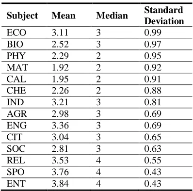
Table-1. Statistical measure of location
Subject Mean Median Standard Deviation
ECO 3.11 3 0.99
BIO 2.52 3 0.97
PHY 2.29 2 0.95
MAT 1.92 2 0.92
CAL 1.95 2 0.91
CHE 2.26 2 0.88
IND 3.21 3 0.81
AGR 2.98 3 0.69
ENG 3.36 3 0.69
CIT 3.04 3 0.65
SOC 2.81 3 0.63
REL 3.53 4 0.55
SPO 3.76 4 0.43
ENT 3.84 4 0.43
Descriptive statistics of the data, as depicted by Table 1, show that ENT, SPO, REL, ENG, IND,
and ECO are subjects whose average are high, i.e., the proportion of 4-mark is higher than that of other marks. While, CAL and MAT are subjects with the lowest average. It is also shown by this
table that ECO, BIO, PHY, MAT, and CAL are subjects with the largest variance and ENT and SPO are those with the lowest. Further description by boxplot shows that ECO, CIT, AGR, CAL, and MAT have symmetric distribution pattern, ENG, IND, PHY, and CHE have positive
distribution pattern, and the remaining subjects have negative distribution pattern. Moreover,
calcu-lation of Pearson correcalcu-lation matrix indicates that almost all variables have p-values less than 1
percent, which shows significant correlation between subjects. In particular, CAL and MAT possess the most correlated subjects, while SPO and ENT provide the most uncorrelated ones. The former fact is obvious, since MAT is a prerequisite for enrolling CAL.
B2 Method
Procedures in B2 method are simplification of those in B1 method, where an analysis based on
principal component is performed only once. The procedure begins by doing PCA over data
matrix. If we decide to retain a number of variables, then weight coefficients with the biggest
magnitude are selected from the last principal components, and linked to corresponding
B4 Method
Similar to B2 method, B4 method needs only one step PCA, but the procedures are now backward.
We start by doing PCA over data matrix. Selection process is performed by choosing
coefficients with the biggest magnitude from the first principal components, and compared each
other starting from the first component.
PCA-PA Method
After performing PCA over data matrix , we construct a score matrix from the first
principal components which represents the data structure. The matrix constitutes as a base
configuration for comparison with other configurations. Next we remove a column of
consecutively and accomplish a PCA over reduced data matrix to produce , where denotes
an score matrix obtained from PCA by removing i-th column of We then compare
over the base configuration by using PA to provide a goodness of fit measure. Variable
corresponds to i-th column which has smallest goodness of fit coefficient is excluded. We rerun the
procedure until the remaining variables. These selected variables represent all variables of
the data.
PA Method
By this method we apply directly procrustes analysis to select variables. Obviously, this is simpler
than previous ones. We first replace one column of consecutively by a column of zeros. We then
match this new matrix up to the original matrix Respective variable that provides smallest
goodness of fit coefficient is excluded. We repeat the process until the remaining variables.
Efficiency Score
An efficiency measure is then needed to justify whether a certain method is considerably more
efficient than others in representing the original data. (Al Kandari and Jolliffe, 2001; Al Kandari
percentage of variation which can be explained by the first pricipal components constructed from
selected variables, whose expression is provided in the previous section. In this study, efficiency
score is measured according to procrustes distance spanned by the matrices. Suppose that is the
original data matrix and is a configuration obtained by keeping variables of . We define by
and the corresponding PCA score matrices related to and , respectively. We here assume
that is the best approximation for Then, the efficiency score is calculated according to the
following formula
Efficiency score varies between 0 and 100 percent. Higher score reveals more efficient and thus
closer similarity between configurations.
RESULT AND DISCUSSION
Based on data exploration, the number of selected variables is not determined by a certain
eigenvalue, rather we follow a criterion proposed by Jolliffe (1972), where is selected such that
the variables can explain at least 80 percent of the variation of the data. It means we keep 8 of 14 variables. This, however, is coincident with the number of departments offering the subjects. For
PCA-PA based methods, we use the first two principal components, i.e., for the analysis,
since they can explain up to 80 percent of the variation of the data.
Table 2 gives the result of variables selection by using four methods in term of selected and
excluded subjects. All the methods show an almost consistent outcome, where BIO, ECO, IND, and AGR are subjects that always selected by all four methods, whereas, MAT, PHY, CHE, and CIT are recommended by three methods. BIO and ECO are two subjects with highest variances and
thus contribute more effects on the variation. Especially for BIO, it is a subject selected by all methods in the first priority. On the other side, ENT, SOC, REL, and SPO are subjects that always
variances than others, hence considerably having less contribution to the variation of the data.
Another obvious fact confirmed by the result relates to CAL and MAT. Except by PCA-PA method, these two subjects show a reverse conduct. If CAL is included then MAT is excluded, and vice versa. It can be understood, since these subjects have similar characteristics due to a high
correlation and one is prerequisite for another.
In particular, six of eight subjects selected by B2 methods are also selected by B4 method. It means that B2 and B4 methods share 75 percent of similarity. PCA and PA methods have also shown similar facts even though PA is much simpler, where they endorse seven mutual selected subjects,
equivalent to 87.5 percent of similarity. From its straightforwardness, PA method is preferably recommended. From the efficiency point of view all the methods are efficient and show
insignificant differences, since all provide high and similar scores. They are more than 99 percent.
Table-2. Result of variables selection by four methods
B2 B4 PCA-PA PA
Included subjects BIO, ECO, PHY,
IND, ENG, MAT, AGR, CIT
BIO, CAL, ECO, IND, CIT, CHE, AGR, ENG
BIO, ECO, PHY, IND, CAL, CHE, MAT, AGR
BIO, ECO, PHY, IND, CHE, MAT, AGR, CIT
Excluded subjects
ENT, SOC, REL, CAL, SPO, CHE
REL, PHY, ENT, MAT, SPO, SOC
ENT, SPO, REL, SOC, CIT, ENG
ENT, SPO, REL, SOC, CAL, ENG
Efficiency score 99.61% 99.21% 99.24% 99.56%
CONCLUDING REMARK
We have implemented a series of variable selection methods based on principal component and
procrustes analyses. The methods have been applied to the assessment of educational data. It has been shown that all the methods provide consistent results. Even though it is not presented in this paper, the methods have been implemented to other situations, where they include of keeping only
7 subjects instead of 8, using the first 3 principal components instead of 2, and utilizing the previous academic year data, i.e., the 2008/2009 data. In fact, all the cases perform minor
differences with the current result. The result of this research can be benefited by the university management in decision making, particularly in courses mapping and student clustering.
REFERENCE
Al Kandari, N.M. and I.T. Jolliffe, 2001. Variable selection and interpretation of covariance principal component. Journal of Statistical Computation and Simulation 30(2): 339-354.
Bakhtiar, T. and Siswadi., 2011. Orthogonal procrustes analysis: Its transformation arrange¬ment and minimal distance. International Journal of Mathematics and Statistics 20(M11): 16-24.
Beale, E.M.L., M.G. Kendal and D.W. Mann, 1967. The discarding of variables in multi¬variate analysis. Biometrika 54: 357-366.
Digby, P.G.N. and R.A. Kempton, 1987. Multivariate analysis of ecological communities. New York: Chapman & Hall: .New York.
George, E.I., 2000. The variable selection problem. Journal of the American Statistical Association, 95: 1304-1308.
Gower, J.C. and G.B. Dijksterhuis, 2004. Procrustes problem. New York: Oxford University Press: New York.
Hurley, J.R. and R.B. Cattell, 1962. The procrustes program: Producing direct rotation to test a hypothesized factor structure. Behavioral Sciences 7: 258-262.
Jolliffe, I.T., 1972. Discarding variable in principal component analysis-i: Artificial data. Applied Statistics 21: 160-173.
Jolliffe, I.T., 2002. Principal component analysis. 2nd Edn., New York: Springer-Verlag: New York.
King, J.R. and D.A. Jackson, 1999. Variable selection in large environmental data sets using principal component analysis. Environmetrics, 10: 67-77.
Sibson, R., 1978. Studies robustness of multi¬di¬mensional scaling: Procrustes statistics. Journal of the Royal Statistical Society B, 40: 234-238.
Siswadi. and T. Bakhtiar, 2011. Goodness of fit of biplots via procrustes analysis. Journal of Mathematical Sciences 52(2): 191-201.