ABSTRACT
LEE, HAN NA. Inference for Eigenvalues and Eigenvectors in Exponential Families of Random Symmetric Matrices. (Under the direction of Dr. Armin Schwartzman.)
Diffusion tensor imaging (DTI) data contains a3×3positive definite random matrix at every voxel (3D pixel). Motivated by the anatomical interpretation of the data, it is of interest to investigate the eigenvalues and eigenvectors of the mean parameter. This dissertation focuses on theory and methodology for analyzing matrix-variated data, based on the inference for the eigenstructure of the mean parameter.
In particular, a matrix-variate exponential family of distributions is presented for random positive definite matrices. Two particular examples of interest in this family that are developed in detail are the matrix-variate gaussian distribution and the matrix gamma distribution. An orthogonal equivariance property of the matrix-variate exponential family is investigated, and estimation and testing procedures for eigenvalues and eigenvectors of the mean matrix are derived. These estimation and testing procedures are carried out both in the one-sample and two-sample problems.
The dissertation is organized as follows. We define a matrix-variate exponential family and establish the properties of this family. Then, we estimate the eigenvalues and eigenvectors of the mean parameter M
under several restrictions, such as fixed eigenvalues and fixed eigenvectors. Using the likelihood of the ex-ponential family defined in Chapter 2, maximum likelihood estimates of eigenvalues and eigenvectors are derived. According to the assumption we make for the eigenstructure, MLEs of eigenvalues and eigenvec-tors can be different. These assumptions for the eigenstructure are tested by likelihood ratio tests; therefore, test statistics for the hypotheses related to these assumptions are also derived.
Estimation and testing procedures for the eigenstructure of the mean parameters in the two-sample problem are also investigated. In two-sample cases, we are focusing on the comparison of two groups. Thus, the restriction for the eigenstructures are based on this comparison.
Although our research is focused on the inference for the mean parameter, assumptions on the nuisance parameters can affect estimation and testing. Thus, a section of this dissertation addresses the handling of nuisance parameters of the matrix-variate gaussian distribution and the matrix gamma distribution.
Inference for Eigenvalues and Eigenvectors in Exponential Families of Random Symmetric Matrices
by Han Na Lee
A dissertation submitted to the Graduate Faculty of North Carolina State University
in partial fulfillment of the requirements for the Degree of
Doctor of Philosophy
Statistics
Raleigh, North Carolina 2016
APPROVED BY:
Dr. David Dickey Dr. Arnab Maity
Dr. Ana-Maria Staicu Dr. Jack Silverstein
DEDICATION
BIOGRAPHY
ACKNOWLEDGEMENTS
First, I would like to express my first and deepest gratitude to my advisor, Dr. Armin Schwartzman. It has been a pleasure working with you. I am grateful for your patience, respect, and warm concern. Without your guidance and financial and emotional support, I would not have been able to complete my study successfully.
I am especially grateful to Drs. David Dickey, Arnab Maity, Ana-Maria Staicu and Jack Silverstein for being my committee members. I greatly appreciate constructive feedback they have provided. I also want to thank to Dr. Huixia Judy Wang, my academic advisor. Her valuable advice and warm words were great help to me. Also, I would like to thank Drs. Kim Weems and Howard Bondell for their great help as a graduate program director.
I would like to thank to my friends in the department. It was a great time with you : To Eun Jeong, Janet, Mi, Meng, Kehui, Soyoung, Bongseok, Marcela, and many others; thank you!
I would like to express my deepest gratitude to my dearest family in Korea, Mom, Dad, and my brother. Also, I am really grateful to my great husband David Ha, my precious daughter Ellen, and parents-in-law. Your love and emotional support have been my biggest strength. It made me possible to complete my re-search work.
TABLE OF CONTENTS
List of Figures . . . vii
Chapter 1 Introduction . . . 1
Chapter 2 Exponential Families of Symmetric Variate Random Matrices . . . 6
2.1 Definition . . . 6
2.2 Expected value and Covariance Matrix ofT(Y) . . . 7
2.3 Orthogonal equivariance of the exponential family . . . 11
2.4 Eigenvalue Parameterization . . . 14
Chapter 3 Maximum Likelihood Estimators in the One-sample Problem . . . 17
3.1 Likelihood for estimating M . . . 17
3.2 Inference forM: MLE and Asymptotic distribution . . . 17
3.3 Inference forU : MLE and Asymptotic distribution . . . 18
3.4 Inference forD: MLE and Asymptotic distribution . . . 22
3.5 MLE of Eigenvectors and Eigenvalues with Known Multiplicities . . . 25
Chapter 4 Testing in One-sample Problems. . . 27
4.1 Full matrix Test . . . 27
4.2 Test of eigenvectors with fixed eigenvalues in a non-increasing order . . . 28
4.3 Test of eigenvalues with unordered eigenvectors . . . 28
4.4 Test of eigenvectors and eigenvalues with known multiplicities . . . 29
Chapter 5 Estimation of eigenstructures in the Two-Sample Case . . . 31
5.1 Estimation under the same nuisance parameter assumption . . . 31
5.2 Estimation under the different nuisance parameters . . . 33
Chapter 6 Testing for eigenstructures in the Two-Sample Case . . . 36
6.1 Full Matrix test . . . 36
6.2 Testing for the eigenvectors . . . 37
6.3 Testing for the eigenvalues . . . 38
Chapter 7 Estimating Nuisance Parameters . . . 40
7.1 Gaussian distribution with spherical covariance matrix . . . 40
7.1.1 Test of Sphericity of Covariance matrices . . . 40
7.1.2 Estimating Covariance parameters in the one-sample case . . . 41
7.1.3 Estimating Covariance parameters in the two-sample case . . . 42
7.2 Matrix Gamma Distribution . . . 43
7.2.1 Estimating shape parameters in the one-sample case . . . 43
7.2.2 Estimating shape parameters in the two-sample case . . . 44
Chapter 8 Numerical Study . . . 45
8.1.1 Distribution ofUˆ andDˆ in the one-sample case . . . 45
8.1.2 Null distribution of test statistics . . . 45
8.1.3 Statistical Power of Tests . . . 46
8.1.4 Estimation of nuisance parameters . . . 48
8.2 Simulation Results . . . 48
8.2.1 Distribution of MLEs . . . 48
8.2.2 Distribution of P-values . . . 50
8.2.3 Statistical Power of Tests . . . 52
8.2.4 Multiplicity test . . . 60
8.2.5 Estimation of other parameters . . . 61
Chapter 9 Real Data Example . . . 65
9.1 Data description . . . 65
9.2 Model checking . . . 65
9.2.1 Model fit . . . 65
9.2.2 Model checking for the Gaussian model . . . 69
9.3 Analysis . . . 71
9.3.1 Gaussian distribution . . . 71
9.3.2 Log-normal distribution . . . 72
9.3.3 Matrix Gamma distribution . . . 73
9.3.4 P-value Maps . . . 75
Chapter 10 Summary and Discussion. . . 79
10.1 Summary . . . 79
10.2 Discussion . . . 79
References . . . 81
Appendix . . . 83
Appendix A Properties needed for the proof of Theorems . . . 84
A.1 Derivation of derivative rules in Example 2.2.2. . . 84
A.2 Derivative of a scalar function with respect to a diagonal matrix . . . 85
LIST OF FIGURES
Figure 8.1 The distribution ofAˆ: one-sample Gaussian case, withn= 200. . . 49 Figure 8.2 The distribution ofAˆ: one-sample matrix gamma case, withn= 200. . . 49 Figure 8.3 The distribution ofDˆ : one-sample Gaussian case, withn= 200. . . 49 Figure 8.4 The asymptotic distribution ofDˆ : one-sample matrix gamma case, withn= 200. . 50 Figure 8.5 The exact distribution ofDˆ : one-sample matrix gamma case, withn= 200.
Com-pared with gamma distribution. . . 50 Figure 8.6 Distribution of p-values for hypothesis testing scenarios: one-sample case, withn=
100. . . 51 Figure 8.7 Distribution of p-values for hypothesis testing scenarios: two-sample case, with
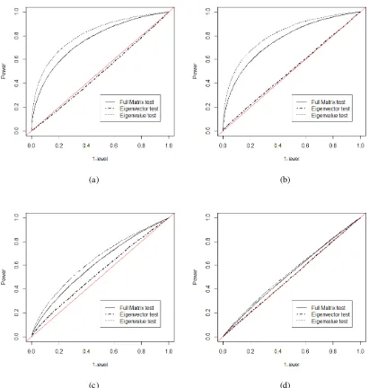
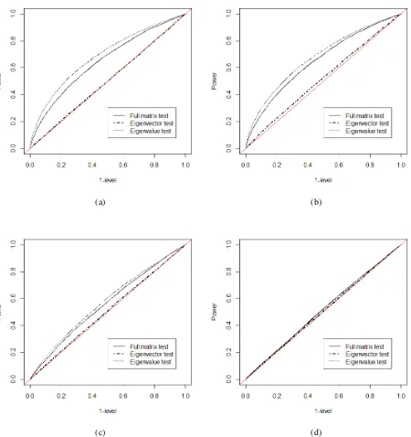
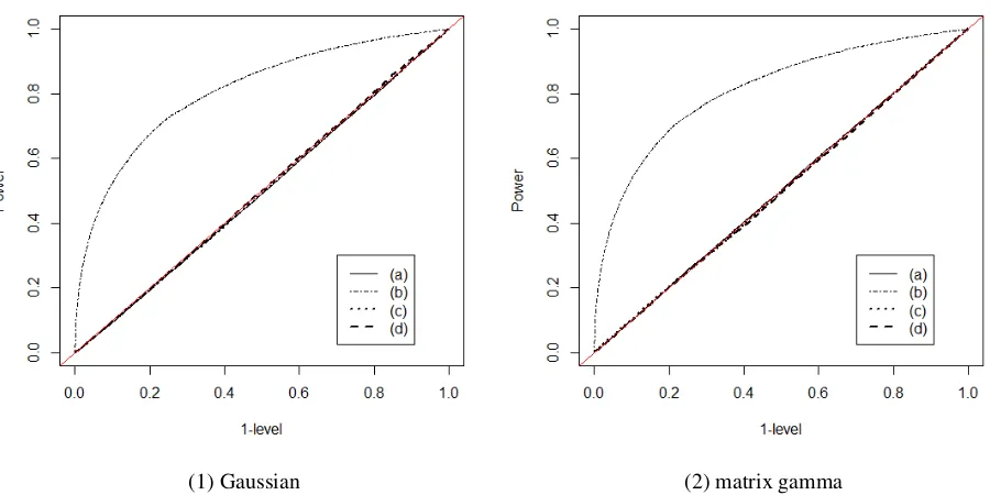
n1 =n2 = 100. . . 51 Figure 8.8 ROC curves for eigenvalue changes: one-sample case, withn= 50, Gaussian
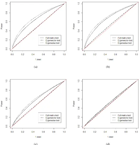
sam-ple. Four eigenvalue-changing matrices are chosen as (a)∆D=Diag(0.8,0.8,0.4), (b) ∆D = Diag(0.8,−0.8,0.4), (c) ∆D = Diag(−0.4,−0.4,0.4), (d) ∆D = Diag(0.2,0.2,0.2). . . 52 Figure 8.9 ROC curves for eigenvalue changes: one-sample case, with n = 50, Wishart
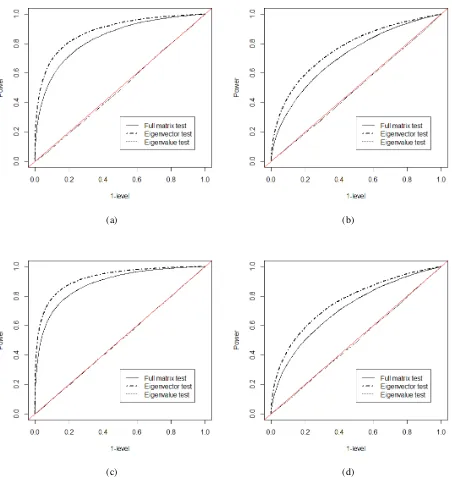
sam-ple. Four eigenvalue-changing matrices are chosen as (a)∆D=Diag(0.8,0.8,0.4), (b) ∆D = Diag(0.8,−0.8,0.4), (c) ∆D = Diag(−0.4,−0.4,0.4), (d) ∆D = Diag(0.2,0.2,0.2). . . 53 Figure 8.10 ROC curves for eigenvector changes: one-sample case, withn= 50, Gaussian
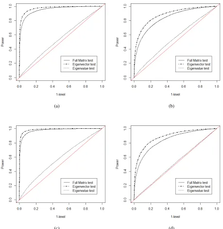
sam-ple. Four unit vectors for rotation matrices are chosen as (a)a= (1/√3,1/√3,1/√3), (b)a = (1,0,0), (c)a= (0,1/√2,1/√2), (d)a = (1/√2,0,−1/√2). The angle
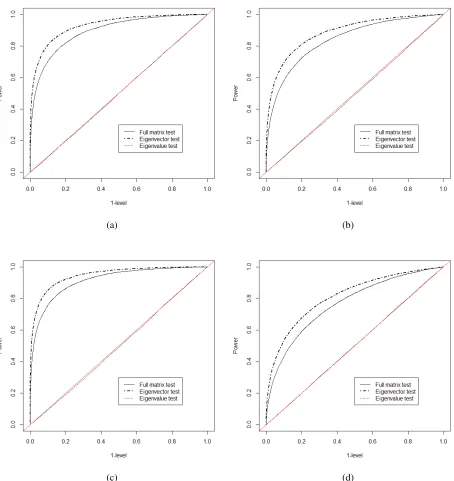
θ=π/12is fixed for all cases. . . 54 Figure 8.11 ROC curves for eigenvector changes: one-sample case, withn= 50, Wishart
sam-ple. Four unit vectors for rotation matrices are chosen as (a)a= (1/√3,1/√3,1/√3), (b)a = (1,0,0), (c)a= (0,1/√2,1/√2), (d)a = (1/√2,0,−1/√2). The angle
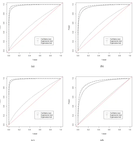
θ=π/12is fixed for all cases. . . 55 Figure 8.12 ROC curves for eigenvalue changes: two-sample Gaussian case, withn1 =n2 = 50.
Four eigenvalue-changing matrices are chosen as (a) ∆D = Diag(0.8,0.8,0.4), (b) ∆D = Diag(0.8,−0.8,0.4), (c) ∆D = Diag(−0.4,−0.4,0.4), (d) ∆D = Diag(0.2,0.2,0.2). . . 56 Figure 8.13 ROC curves for eigenvalue changes: two-sample Wishart case, withn1 =n2= 50.
Four eigenvalue-changing matrices are chosen as (a) ∆D = Diag(0.8,0.8,0.4), (b) ∆D = Diag(0.8,−0.8,0.4), (c) ∆D = Diag(−0.4,−0.4,0.4), (d) ∆D = Diag(0.2,0.2,0.2). . . 57 Figure 8.14 ROC curves for eigenvector changes: two-sample Gaussian case, withn1 = n2 =
50. Four unit vectors for rotation matrices are chosen as (a)a= (1/√3,1/√3,1/√3), (b)a = (1,0,0), (c)a= (0,1/√2,1/√2), (d)a = (1/√2,0,−1/√2). The angle
θ=π/12is fixed for all cases. . . 58 Figure 8.15 ROC curves for eigenvector changes: two-sample Wishart case, withn1 =n2 = 50.
Four unit vectors for rotation matrices are chosen as (a)a= (1/√3,1/√3,1/√3), (b)a = (1,0,0), (c)a= (0,1/√2,1/√2), (d)a = (1/√2,0,−1/√2). The angle
Figure 8.16 ROC curves for multiplicity test: Gaussian and matrix gamma withn = 50. Four eigenvalue-changing matrices are chosen as (a)∆D=Diag(0.8,0.8,0.4), (b)∆D= Diag(0.8,−0.8,0.4), (c)∆D=Diag(−0.4,−0.4,0.4), (d)∆D=Diag(0.2,0.2,0.2). 60 Figure 8.17 ROC curves for multiplicity test: Gaussian and matrix gamma withn = 50. Four
eigenvector-changing matrices are chosen as (a)a= (1/√3,1/√3,1/√3), (b)a=
(1,0,0), (c)a= (0,1/√2,1/√2), (d)a= (1/√2,0,−1/√2). Figure (a) . . . 61
Figure 8.18 The distribution ofσˆ2: one-sample Gaussian case, withn= 100. . . 62
Figure 8.19 The distribution ofσˆ212: two-sample Gaussian case, equal covariance assumption, withn1 =n2 = 100. . . 62
Figure 8.20 The distribution ofσˆ12 andσˆ22: two-sample Gaussian case, different covariance as-sumption, withn1=n2 = 100. . . 63
Figure 8.21 The distribution ofαˆ: one-sample Wishart case, withn= 100. . . 63
Figure 8.22 The distribution ofαˆ1 andαˆ2: two-sample Wishart case, withn1 =n2 = 100. . . . 64
Figure 9.1 Histograms of Mardia Test statistics to check normality . . . 66
Figure 9.2 Histograms of Mardia Test statistics to check log-normality . . . 66
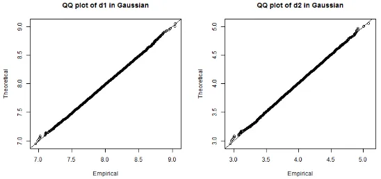
Figure 9.3 Chi-square qq plot at voxel number=1020; Left : Boys, Right : Girls . . . 67
Figure 9.4 Chi-square qq plot at voxel number =1000; Left : Boys, Right : Girls. . . 67
Figure 9.5 Histograms of K-S P-values to check the gamma distribution assumption for boys . . 68
Figure 9.6 Histograms of K-S P-values to check the gamma distribution assumption for girls . . 68
Figure 9.7 Box’s M test for the equality of covariance matrices. . . 69
Figure 9.8 The test of spherical covariance : Gaussian distribution . . . 70
Figure 9.9 The test of multiplicity :k= 1 . . . 71
Figure 9.10 The test of multiplicity :k= 2 . . . 72
Figure 9.11 The p-value level plot in scale−log10(p)for multiplicity test at slicez= 49:k= 1, matrix gamma distribution . . . 72
Figure 9.12 The p-value level plot in scale−log10(p)for multiplicity test at slicez= 49:k= 2, matrix gamma distribution . . . 73
Figure 9.13 The distribution of p-values: two-sample Gaussian distribution with arbitrary covari-ance, using weighted chi-square distribution . . . 73
Figure 9.14 The distribution of p-values : two-sample log-normal distribution with arbitrary co-variance, using weighted chi-square distribution . . . 74
Figure 9.15 Histogram oflog|αˆ1−αˆ2| ˆ α1 . . . 74
Figure 9.16 Scatterplot ofαˆ1andαˆ2. . . 75
Figure 9.17 The distribution of p-values: two-sample Wishart distribution . . . 75
Figure 9.18 The p-value level plot in scale−log10(p)at slicez= 40: Gaussian distribution . . . 76
Figure 9.19 The p-value level plot in scale−log10(p)at slicez= 49: Gaussian distribution . . . 76
Figure 9.20 The p-value level plot in scale−log10(p)at slicez= 40: log-normal distribution . . 77
Chapter 1
Introduction
Consider ap×prandom symmetric matrixY from some probability density functionf(Y;M), whereM
is the mean parameter of this density. Here,Y andM are in the set ofp×psymmetric matrices, denoted by
Sp. Our goal is to estimate and test hypotheses about the mean parameterM, with some assumptions on the distribution of random matrixY and restrictions on the parameter space, such thatM is in certain subsets ofSp. In particular, our research is focused on estimating and testing the eigenvalues and eigenvectors of
M, when we have restrictions such that the eigenvalues of M are fixed, the set of eigenvectors of M is fixed with consideration for the order, and the eigenvalues ofM have some specific multiplicities. For these inference problems, the observations are drawn from one population as a random sample.
view-point, eigenvalues of the diffusion tensor represent information about the type of tissue and its condition, and eigenvectors provide information about the spatial orientation of neural fibers (Basser, Mattiello, and LeBi-han, 1994). Thus, statistical inference for the eigenstructure of random symmetric matrices can be useful in the analysis of DTI data (Schwartzman, 2006; Zhu et al., 2007; Schwartzman et al., 2008; Schwartzman et al., 2010).
Another motivating example can be found in social science, related to principal component analysis (PCA) and factor analysis (FA) in classical multivariate analysis. PCA is a method for reorienting multivariate data to explain as much of the information as possible with a small number of new variables called principal components (PC) (Mardia, Kendt, and Bibby, 1979, page 213; Lattin, Carrol, and Green, 2003, page 121; Johnson and Wichern, 2007, page 430). In PCA, the eigenvalues of the covariance matrix or correlation ma-trix represent the amount of information explained by each principal component, while eigenvectors show us the direction of variability. Factor analysis, which was originally developed by a psychologist (Spearman, 1904; Bartlett, 1937), is a method to describe the covariance relationships among many variables with a small number of unobservable (latent) variables called factors (Mardia, Kendt, and Bibby, 1979, page 255; Johnson and Wichern, 2007, page 481). To estimate the factor model, the principal components method described above is commonly used.
In practice, FA has contributed to advancing psychological research, which has been used extensively as a data analytic technique for examining patterns of interrelationship, data reduction, hypothesis testing, and so on (Rummel, 1970; Ford, Mccallum, and Tait, 1986; Molenaar et al., 1992; Fabrigar et al., 1999). Inferences for eigenstructure of covariance matrices are relavant to FA. For instance, if we want to compare the pattern of test scores of several different groups in terms of common factors, the effect of common factors can be examined by testing equality of eigenvectors between the covariance matrices of the groups. Moreover, FA is also commonly used in macroeconometrics. In dynamic factor models, for example, multivariate time-series data is handled where the covariance matrix varies over time. As such, these time-varying multiple covariance matrices can be compared in terms of factors by comparing their eigenvalues and eigenvectors (Forni et al., 2000; Del Negro and Otrok, 2008).
distributions.
There are several decomposition methods applied to investigate the structure of covariance matrix. We can find several works in the literature that mention decomposition methods used in the estimation of a covari-ance matrix, such as Varicovari-ance-correlation Decomposition (Barnard et al., 2000), Spectral Decomposition (Boik, 2002), and Cholesky Decomposition (Pourahmadi, 1999; Smith and Kohn, 2002; Chen and Dunson, 2003). Among these decompositions, Cholesky Decomposition is also commonly used to examine the struc-ture of covariance matrices, especially in Time Series Analysis and Longitudinal Data Analysis. Cholesky Decomposition also provides a statistically meaningful reparameterization of a covariance matrix (Pourah-madi, 1999; Pourah(Pourah-madi, 2007). In DTI, however, the eigenvalues and eigenvectors of a covariance matrix also have their own anatomical meanings. Since our work is motivated by DTI, we use a spectral decompo-sition.
There are a few works about inferences for the eigenstructure ofp×prandom symmetric matrices when the sample data is assumed to be from a specific distribution. Mallows (1961) presented work about linear hypotheses involved in testing the eigenvectors of a single matrix in the case of a Gaussian distribution with orthogonally invariant covariance structure. This reference provides the concept of orthogonally invariant covariance structure, which means the distribution of a random matrix Y is the same as that of QY QT
different distributions.
We have assumed a parametric distribution for the matrix variate data to make inferences for the eigenstruc-ture of symmetric random matrix using MLE and LRT, since this assumption has all the convenience of parametric models in terms of analytic expressions and can be efficiently applied to each of tens of thou-sands of voxels in DTI data. A symmetric matrix-variate Gaussian distribution with orthogonally invariant covariance can be considered for a symmetric random matrixY. Otherwise, we can assume the distribu-tion of a symmetric random matrix as Wishart distribudistribu-tion, since this is a natural model to consider for covariance matrices. Furthermore, we consider an exponential family, which includes many common dis-tributions such as matrix-variate Gaussian, exponential, matrix gamma, and Wishart distribution (Fisher, 1934; Pitman, 1936; Koopman, 1936). Exponential families for univariate and multivariate data and infer-ence methods for them are well-known (Mardia, Kent, and Bibby, 1979, page 45; Lehmann and Casella, 1998, page 23; Casella and Berger, 2001, page 217). Analogous to other multivariate exponential families, we define a matrix-variate version of exponential family. Analytical calculations are possible if the distribu-tion is assumed to be equivariant under orthogonal transformadistribu-tions. With this exponential family form, we can estimate and test the eigenstructure ofM in the general exponential family using MLE and LRT. Then we can apply the result to each specific distribution.
In order to find analytical solutions, we define the concept of orthogonally equivariant (OE) family of dis-tributions. OE family is a group family of probability distributions that is generated by the group action (rotation and reflection) of the orthogonal matrix group. As our problem is focused on the inferences for eigenvalues and eigenvectors, which are related to orthogonal matrices, by assuming that the probability distributions considered are in the OE family, we can make inferences for the eigenstructures of mean pa-rameters more explicitly.
In our problem, the parameter space is, in general, a submanifold of Euclidean space. For instance, requiring the eigenvalue matrix to be diagonal creates a linear submanifold in the Euclidean space of square matri-ces of sizep. On the other hand, the constraint that the eigenvector matrix should be orthogonal defines an algebraic curved submanfiold. For this reason, we cannot use the usual method for calculating MLEs in a Euclidean space. Instead, we obtain the critical points by finding the score function in two ways: using the projection of the unrestricted gradient onto the manifold or tracing a curve directly on the manifold. Once we have the score function by either method, we obtain critical points by setting the score function equal to 0. These points maximize the likelihood because of convexity, so we get the MLEs. Using the MLEs derived from this procedure, we perform LRTs for the hypotheses related to the constraints on the eigenstructure of the parameter matrixM.
Chapter 2
Exponential Families of Symmetric Variate
Random Matrices
2.1
Definition
Suppose the probability density of ap×psymmetric random matrixY can be written in the form
f(Y; Θ) =H(Y)e{tr(η(Θ)T(Y))−K(η(Θ))} (2.1) whereΘis a parameter matrix. Assume thatK(η)is twice differentiable. Then,Y is said to belong to an exponential family of distributions, and we call (2.1) the canonical form of the exponential family.
In our research, we focus on estimating and testing the mean parameterM =E(T(Y)), where Y, M,T(Y), andη(M)are symmetric. Any other parameters, such as variance, scale parameter, shape parameter and so on, are considered as nuisance parameters. Therefore, we rewrite (2.1) as a function ofM, which has the form
f(Y;M) =H(Y)e{tr(η(M)T(Y))−K(η(M))}. (2.2)
Example 2.1.1. In the case of symmetric matrix variate Gaussian distribution with spherical covariance (Schwartzman et al, 2008), denoted asY ∼Npp(M, σ2Iq), the probability density function is
f(Y;M) = 1 (2π)q2σq
e−2σ12tr{(Y−M)
2}
=H(Y)e2σ12tr(2Y M−M
2)
whereq = p(p2+1). As the pdf of Gaussian distribution can be written in the canonical form, it is an expo-nential family. In this case, we have
H(Y) = 1 (2π)q2σq
e−2σ12tr(Y2), η(M) = M
σ2, T(Y) =Y, K(η(M)) = 1 2σ2tr(M
Example 2.1.2. In the case of matrix gamma distribution, we have the pdf
f(Y;M) = |M|
−α
α−αpΓ p(α)
|Y|α−p+12 eαtr(−(M−1Y))=H(Y)eα{−tr(M−1Y)−log|M|}.
whereΓp(α)is the multivariate gamma function defined as
Γp(α) = πp(p−1)/4 p Y
j=1 Γ
α+1−j 2
.
As the pdf of matrix gamma distribution can be rewritten as the canonical form of exponential family, it is an exponential family. In this case, we have
H(Y) = |Y| α−p+12
α−αpΓ p(α)
, η(M) =−αM−1, T(Y) =Y, K(η(M)) =αlog|M|.
2.2
Expected value and Covariance Matrix of
T
(Y
)
To obtain the general form of the moments ofT(Y)in the exponential family, let us start from the definition of probability density function. Before we start, we will use a vectorization operator for any symmetric matrixXdefined in (Schwartzman et al, 2008), such that
vecd(X) = (diag(X)T,√2offdiag(X)T)T
where the diag(X)operator is defined as the vector whose elements are the diagonal elements ofX, and offdiag(X)is defined as the vector whose elements are the off-diagonal elements ofX. Using this operator, the correlation between diagonal elements and off-diagonal elements of a matrix is seen more clearly. In addition, by multiplying √2 by the off-diagonal elements, the equationvecd(A)Tvecd(B) = Tr(AB) is satisfied, so we can easily present the trace of a matrix product as an inner product of two vectors. We can also connect this definition tovec operator, by choosing a duplication matrixDsuch thatvec(Y) = Dvecd(Y). For example, we have a duplication matrixDforp= 3such that
D=
1 0 0 0 0 0 0 0 0
0 0 0 0 1 0 0 0 0
0 0 0 0 0 0 0 0 1
Such a duplication matrix always exists for anyp, although it is generally not unique.
Theorem 2.1. The expected value and covariance matrix ofT(Y)are as follows. (i)M =E[T(Y)] = ∂K∂η(η(M(M))).
(ii) Cov[vecd(T(Y))] = ∂vecd(η(∂M2K))(∂ηvecd((M))η(M))T. P roof. We will use two methods to prove this theorem.
M ethod1. Using the moment generating function (i) The moment generating function can be obtained as
MT(S) = E{etr(ST(Y))} =
Z
etr(ST(Y))H(Y)e{tr(ηT(Y))−K(η)}dY
= eK(S+η)−K(η)
Z
H(Y)e{tr((S+η)T(Y))−K(S+η)}dY
= eK(S+η)−K(η).
where the domain ofSis a set of symmetric matrices. Taking derivative of the moment generating function with respect to S, and substitutingS= 0, we have
E(T(Y)) = ∂MT(S)
∂S S=0 = ∂ ∂Se
K(S+η)−K(η)
S=0 = eK(S+η)−K(η)∂K(S+η)
∂S S=0 = ∂K(S+η)
∂S S=0 Setting S + η = ν, ∂∂vecdvecd(T(Sν)) = Iq and ∂vecd(η)
T
∂vecd(ν) = Iq. Thus,
∂K(S+η) ∂vecd(S) =
∂K(ν) ∂vecd(ν)
∂vecd(ν)T
∂vecd(S) = ∂K(ν)
∂vecd(ν) =
∂K(ν) ∂vecd(η) ∗
∂vecd(η)T
∂vecd(ν) =
∂K(ν)
∂vecd(η). Using this fact, we have
∂K(S+η)
∂S =
∂K(S+η) ∂η . Thus, E(T(Y)) = ∂K(∂ηS+η)|S=0= ∂K∂η.
(ii) To find the variance, we need the second moment. Let us compute the derivative of the moment generat-ing function with respect tovecd(S)instead ofS. Then, we have
∂MT(S)
∂vecd(S) =
∂ ∂vecd(S)e
K(S+η)−K(η)
= eK(S+η)−K(η)∂K(S+η) ∂vecd(S) .
To obtain the second moment, take the derivative of ∂MT(S)
∂2MT(S)
∂vecd(S)∂vecd(S)T =
∂2
∂vecd(S)∂vecd(S)T[e
K(S+η)−K(η)]
= eK(S+η)−K(η)
∂K(S+η)
∂vecd(S)
∂K(S+η)
∂vecd(S)T
+eK(S+η)−K(η) ∂
2K(S+η)
∂vecd(S)∂vecd(S)T
Using the relationship∂K(∂SS+η) = ∂K(∂ηS+η) shown in part (i), we have
∂2M T(S)
∂vecd(S)∂vecd(S)T = e
K(S+η)−K(η)
∂K(S+η)
∂vecd(η)
∂K(S+η)
∂vecd(η)T
+eK(S+η)−K(η) ∂
2K(S+η)
∂vecd(η)∂vecd(η)T
From the above second derivative, we have
E{vecd(T(Y))vecd(T(Y))T}= ∂ 2M
T(S)
∂vecd(S)∂vecd(S)T S=0
= ∂K(η)
∂vecd(η)
∂K(η)
∂vecd(η)T+
∂2K(η)
∂vecd(η)∂vecd(η)T.
Thus, the covariance matrix ofT(Y)is
Cov[vecd(T(Y))] = E{vecd(T(Y))vecd(T(Y))T} −E{vecd(T(Y))}E{vecd(T(Y))}T =
∂K(η)
∂vecd(η)
∂K(η)
∂vecd(η)T
+ ∂
2K(η)
∂vecd(η)∂vecd(η)T −
∂K(η)
∂vecd(η)
∂K(η)
∂vecd(η)T
= ∂
2K(η)
∂vecd(η)∂vecd(η)T.
M ethod2. Using the unit-mass property of pdf.
Another way of proving is to use the fact thatR f(Y; Θ)dY = 1. (i) We have
Z
h(Y)e{(tr(η(M)T(Y))−K(η(M)}dY = 1.
Drawing the function of parameters from the integral, we have
e−K(η(M))
Z
H(Y)e{tr(η(M)T(Y))}dY = 1.
From the above equation, we can deriveR
H(Y)e{tr(η(M)T(Y))}dY =eK(η(M)). Setting
F(η(M)) = Z
H(Y)e{tr(η(M)T(Y))}dY,
Next, we take the derivative with respect toη(M)on both sides. For the convenience, we denoteη =η(M).
∂K
∂η =
∂
∂η[logF(η)]
= 1
F(η)
∂F(η)
∂η
= 1
F(η) Z
T(Y)H(Y)e{tr(ηT(Y))}dY
= R
T(Y)H(Y)e{tr(ηT(Y))}dY F(η)
e−K(η) e−K(η) =
R
T(Y)H(Y)e{tr(ηT(Y))−K(η)}dY
1 = E[T(Y)] =M
(ii) From (i), we have ∂vecd(∂Kη)T =vecd(M)T. Therefore, let us set ∂2K
∂vecd(η)∂vecd(η)T =
∂ ∂vecd(η)
∂
∂vecd(η)T logF(η)
= ∂
∂vecd(η)
1
F(η)
∂F(η)
∂vecd(η)T
= − 1
F(η)2
∂F(η)
∂vecd(η)
dF(η)
∂vecd(η)T + 1
F(η)
∂2F(η)
∂vecd(η)∂vecd(η)T
The first term can be simplified as 1
F(η)2
∂F(η)
∂vecd(η)
∂F(η)
∂vecd(η)T = − 1
F(η)
∂F(η)
∂vecd(η) 1
F(η)
∂F(η)
∂vecd(η)T = −E{vecd(T(Y))}E{vecd(T(Y))}T
using the same logic in (i). Next, the second term can be rewritten as 1
F(η)
∂2F(η)
∂vecd(η)∂vecd(η)T = 1
F(η) Z
vecd(T(Y))vecd(T(Y))TH(Y)evecd(η)Tvecd(T(Y))dY
= R
vecd(T(Y))vecd(T(Y))TH(Y)evecd(η)Tvecd(T(Y))dY F(η)
e−K(η) e−K(η) =
R
vecd(T(Y))vecd(T(Y))TH(Y)evecd(η)Tvecd(T(Y))−K(η)dY
∂2K
∂vecd(η)∂vecd(η)T = − 1
F(η)2
∂F(η)
∂vecd(η)
∂F(η)
∂vecd(η)T + 1
F(η)
∂2F(η)
∂vecd(η)∂vecd(η)T
= −E{vecd(T(Y))}E{vecd(T(Y))}T +E{vecd(T(Y))vecd(T(Y))T} = Cov[vecd(T(Y))].
This is the same as the formula from the first method.
Example 2.2.1. In the case of symmetric matrix variate Gaussian distribution with spherical covariance shown in Example 2.1.1, we have η(M) = Mσ2, T(Y) = Y and K(η(M)) = tr(M
2
2σ2) = tr( σ2η2
2 ) = σ2
2 (vecd(η)
Tvecd(η)). Therefore, E(T(Y)) = ∂K ∂η =σ
2η =Mand Cov(vecd(T(Y))) = ∂2K
∂vecd(η)∂vecd(η)T =
∂ ∂vecd(η)(
∂K ∂vecd(η)T) =
∂
∂vecd(η)(σ2vecd(η)T) =σ2Iq.
Example 2.2.2. In the case of matrix gamma distribution, we haveη(M) = −αM−1, T(Y) = Y, and
K(η(M)) =αlog|M|=αlog| −αη−1|=α{plogα−log| −η|}. So, E(T(Y)) = dK dη =
d
dη{−αlog| −
η|}=−αη−1 =M.
We use the derivative rules ∂∂vecd(vecd(ηη−)T1) = −DT(η
−1⊗η−1)D, described in Appendix A. The covariance matrix has the form
Cov(vecd(Y)) = ∂ 2K
∂vecd(η)∂vecd(η)T =
∂
∂vecd(η)T{−αvecd(η
−1)}
= −α{−DT(η−1⊗η−1)D} = 1
αD
T(M ⊗M)D.
We have entry-wise variance and covariance formula for the matrix gamma case from other book(Gupta and Nagar, 1999), which is actually derived from the wishart distribution by modifying parameters, such that Var(Yij) = 21α(µij2 +µiiµjj)whereµij is the (i, j)th element ofM, and Cov(Yij, Ykl) = 21α(µikµjl+
µilµjk). The above matrix-variate formula provides the same answer.
2.3
Orthogonal equivariance of the exponential family
Orthogonal equivariance is an additional property imposed on the exponential family that facilitates obtain-ing analytical expressions for the MLEs and LLRs considered in this work. To make this explicit, some definitions and assumptions are given first.
Definition 2.1. A square matrix functiona(X) of square matrix argument X is analytic ifa(X) can be represented as the form of convergent power series such thata(X) =P∞
k=−∞ckXkfor some coefficients
ck. In particular, an analytic function is infinitely differentiable.
Definition 2.2. For a square matrixX,
(i) A functiong(X)is orthogonally invariant ifg(X)satisfiesg(RXRT) =g(X)for any orthogonal matrix
R.
(ii) A squared matrix functiong(X)is orthogonally equivariant ifg(X)satisfiesg(RXRT) =Rg(X)RT
for any orthogonal matrixR.
Note that an analytic functiona(X)is orthogonally equivariant, since an analytic function satisfiesa(P XP−1) =
P a(X)P−1for any invertible matrixP and an orthogonal matrixRsatisfies thatR−1=RT.
Definition 2.3. If a pdff(Y;M)safistiesf(Y;M) =f(RY RT;RM RT)for any orthogonal matrixR, the pdf is then said to be an orthogonal equivariant (OE) family.
Assumption2.1. For a density functionf(Y;M)that has the form (2.2), (i)K(∗)andH(∗)are orthogonally invariant functions.
(ii)η(∗)is an analytic function. (iii)T(∗)is an OE function.
Proposition 2.1. Let f(Y;M) have the form (2.2) and suppose that Assumption 2.1 holds. Then, the density ofY is an OE family.
P roof. LetY˜ =RY RT for any orthogonal matrixR. We will obtain the density function ofY˜ by variable transformation. We haveY =RTY R˜ sinceRis an orthogonal matrix, and we havedY˜ =|R|p|RT|pdY = |RRT|pdY =dY using the property that if we haveXandY matrices such thatY =AXBwith nonsin-gular constant p×pmatrices AandB, dY = |A|p|B|pdX (Mathai, 1997, page 31). Thus, the Jacobian of this transformation is|J| = |dY
dY˜| = 1. Therefore, we can find the density ofY˜ as follows. AsT(∗)is orthogonally equivariant andH(∗)is orthogonally invariant,
f( ˜Y) = H(RTY R˜ )exp[tr{η(M)T(RTY R˜ )} −K{η(M)}]∗ |J| = H( ˜Y)exp[tr{η(M)RTT( ˜Y)R} −K{η(M)}]
= H( ˜Y)exp[tr{Rη(M)RTT( ˜Y)} −K{Rη(M)RT}] = H( ˜Y)exp[tr{η(RM RT)T( ˜Y)} −K{η(RM RT)}] = H( ˜Y)exp[tr{η( ˜M)T( ˜Y)} −K{η( ˜M)}]
whereM˜ = RM RT. Note that the density function ofY˜ has the same form as the original one, with the parameter matrix which is rotated with respect toR.
It can be seen that both the spherical Gaussian and matrix-Gamma distributions of examples 2.1.1 and 2.1.2 have OE density functions.
spher-ical covariance can be represented as
f(Y;M) = H(Y)e2σ12tr(2Y M−M
2)
.
withH(Y) = 1 (2π)q2σqe
− 1 2σ2tr(Y
2)
. SettingY˜ =RY RT for some orthogonal matrixR, we have (i)H( ˜Y) = 1
(2π)q2σqe
− 1
2σ2{−tr((RY R T)2)}
= 1 (2π)q2σqe
− 1 2σ2tr(Y
2)
=H(Y).
K(Rη(M)RT) =K(η(RM RT)) = 2σ12tr(RM2RT) = 1
2σ2tr(M2) =K(η(M)). Thus,H(Y)andK(∗)are orthogonally invariant.
(ii)η(M) = Mσ2 is an analytic function.
(iii) We haveT(Y) =Y, which meansT(Y)is orthogonally equivariant.
Thus, all the three assumptions are satistied, so the pdf of Gaussian distribution is an OE family.
Example 2.3.2. In the case of matrix gamma distribution, we have the pdf form
f(Y;M) = H(Y)eα{−tr(M−1Y)−log|M|}.
withH(Y) = |Y|
α−p+12
α−αΓ
p(α). Setting
˜
Y =RY RT for some orthogonal matrixR, (i)H( ˜Y) = |RY RT|α
−p+1
2 α−αΓ
p(α) =
|Y|α−p+12 α−αΓ
p(α) =H(Y).
K(Rη(M)RT) =K(η(RM RT)) =αlog|RM RT|=αlog|M|=K(η(M)). Thus,K(∗)andH(Y)are orthogonally invariant.
(ii)η(M) =−αM−1is an analytic function. (iii)T(Y) =Y is orthogonally equivariant.
Thus, all the three assumptions are satistied, so the pdf of matrix gamma distribution is an OE family.
Corollary 2.1. LetW =RT(Y)RT andM˜ =RM RT for any orthogonal matrixR. Suppose the pdf ofY
is an OE family. Then,
(i) E[W] = ∂K(η( ˜M)) ∂η( ˜M) = ˜M
(ii) Cov[vecd(W)] = ∂2K(η( ˜M))
∂vecd(η( ˜M))∂vecd(η( ˜M))T.
P roof. From the assumption, we have that the pdf f(Y) is orthogonally equivariant. Thus, by obtaining the distribution ofY˜ =RY RT, we can find the mean and covariance ofW =RT(Y)RT. Note that since
T(Y)is a orthogonally equivariant function,W =T( ˜Y). The pdf ofY˜ is
f( ˜Y; ˜M) =H( ˜Y)exp[tr{η( ˜M)T( ˜Y)} −K{η( ˜M)}], (2.3) which also has the exponential family form. Thus, from this pdf, we can get
E(T( ˜Y)) = ∂K(η( ˜M))
Cov[vecd(T( ˜Y))] = ∂
2K(η( ˜M))
∂vecd(η( ˜M))∂vecd(η( ˜M))T, using the result of Theorem 2.1.
Example 2.3.3. In the case of symmetric matrix variate Gaussian distribution with spherical covariance, as shown in Example 2.1.1, we haveη( ˜M) = Mσ˜2,T( ˜Y) = RY RT andK(η( ˜M)) = tr(
˜ M2
2σ2) = tr( σ2η˜2
2 ). Therefore,
E(W) = ∂K(η( ˜M))
∂η( ˜M) =σ
2η( ˜M) = ˜M
Cov(vecd(W)) = ∂
2K(η( ˜M))
∂vecd(η( ˜M))∂vecd(η( ˜M))T =σ 2I
q.
Example 2.3.4. In the case of matrix gamma distribution, we haveη( ˜M) = −αM˜−1,T( ˜Y) = RY RT, andK(η( ˜M)) =αlog|M˜|=α{plogα−log| −η˜|}. Therefore,
E(W) = ∂K(η( ˜M))
∂η( ˜M) =−αη( ˜M)
−1 = ˜M
Cov(vecd(W)) = ∂
2K(η( ˜M))
∂vecd(η( ˜M))∂vecd(η( ˜M))T = 1
αD
T( ˜M⊗M˜)D
Thus, each element ofW has the variance Var(Wij) = 21α(˜µ2ij + ˜µiiµ˜jj)whereµ˜ij is the(i, j)th element ofM˜ =RM RT and Cov(Wij, Wkl) = 21α(˜µikµ˜jl+ ˜µilµ˜jk).
2.4
Eigenvalue Parameterization
Until the previous section, the structure of mean parameterM was not specified. Now, consider the eigen-structure ofM, denoted asM =U DUT, whereDis a diagonal matrix whose elements are eigenvalues of
M andU is an eigenvector matrix corresponding toD. Then, we can rewrite the pdf as a function ofU and
Das
f(Y;U, D) =H(Y)e{(tr(U η(D)UTT(Y))−K(η(D)}. (2.4) The following useful lemma establishes the moments of the random matrixT(Y)rotated by the eigenvec-tors.
Lemma 2.1. Suppose all the assumptions in Corollary 2.1 are satisfied andW =RT(Y)RT. AtR=UT, (i) E(W) = ∂K(η( ˜M))
∂η( ˜M)
R=UT =D.
(ii) Cov(vecd(W)) = ∂2K(η( ˜M)) ∂vecd(η( ˜M))∂vecd(η( ˜M))T
P roof. (i) We will prove this using Corollary 2.1. By proposition 2.1., the pdf ofY is orthogonally equiv-ariant. Therefore, we have
∂K(η( ˜M))
∂η( ˜M) = ˜M .
Assuming thatM =U DUT by eigen decomposition, the expected value ofW can be obtained by evaluating the above equation atR=UT. Thus, we have
∂K(η( ˜M))
∂η( ˜M)
R=UT
= ˜M|R=UT =UTM U =UTU DUTU =D.
(ii) From (i), we can derive that ∂K(η( ˜M))
∂vecd(η( ˜M)) =vecd( ˜M). Therefore, this equation holds;
∂2K(η( ˜M))
∂vecd(η( ˜M))∂vecd(η( ˜M))T =
∂vecd( ˜M)
∂vecd(η( ˜M))T
Using the property of derivatives, ∂vecd(∂vecd( ˜η( ˜MM)))T = [
∂vecd(η( ˜M)) ∂vecd( ˜M)T ]
−1. Here, since the functionηis analytic, we can use the definition of analytic function to find the derivative. Recall
η(M) =
∞
X
k=−∞
ckMk.
Fork >0, we have
d(Mk) = dM ·Mk−1+M·dM·Mk−2+...+Mk−1·dM
vec(d(Mk)) = (Mk−1⊗I)vec(dM) + (Mk−2⊗M)vec(dM) +...+ (I⊗Mk−1)vec(dM)
∂vec(Mk)
∂vec(M)T = (M
k−1⊗I) + (Mk−2⊗M) +...+ (I⊗Mk−1) using matrix differential and property ofvecoperator.
Starting from the equation thatMk·M−k=I, we have
Mk·M−k = I d(Mk)M−k+Mkd(M−k) = 0
d(M−k) = −M−kd(Mk)M−k
vec(d(M−k)) = −(M−k⊗M−k)vec(dMk)
∂vec(M−k)
∂vec(Mk)T =−(M
Now we use the chain rule so that
∂vec(M−k)
∂vec(M)T =
∂vec(M−k)
∂vec(Mk)T ·
∂vec(Mk)
∂vec(M)T.
Next, replacing M into M˜ = U M UT = D, we can see that ∂∂vecvec((MM)kT) is diagonal for all k. Using a
duplication matrixD, we can obtain∂∂vecdvecd((MM)kT) which is still diagonal for allk. Thus,
∂vecd(η( ˜M))
∂vecd( ˜M) is diagonal since it can be represented as the product of diagonal matrices. By taking inverse of this, we can get the covariance matrix ofvecd( ˜M), which is diagonal.
Example 2.4.1. In the case of symmetric matrix variate Gaussian distribution with spherical covariance, we haveη( ˜M) = Mσ˜2,T( ˜Y) = RY RT andK(η( ˜M)) = tr(
˜ M2
2σ2) = tr( σ2η˜2
2 ), as shown in Example 2.3.3. TakingR = UT, we haveM˜ = UTM U = UTU DUTU = D. Therefore, E(W) = σ2η(D) = Dand Cov(vecd(W)) =σ2Iq.
Example 2.4.2. In the case of matrix gamma distribution, we haveη( ˜M) = −αM˜−1,T( ˜Y) = RY RT, andK(η( ˜M)) = αlog|M˜| =α{plogα−log| −η˜|}, as shown in Example 2.3.4. TakingR = UT, we haveM˜ =UTM U =UTU DUTU =D. Therefore, E(W) =−αη(D)−1 =Dand the covariance matrix has the form
Cov(vecd(W)) = 1
αD
T(D⊗D)D
Chapter 3
Maximum Likelihood Estimators in the
One-sample Problem
3.1
Likelihood for estimating M
LetY1, ..., Ynbe a random sample of sizenfrom the density (2.2). In terms of this sample with sizen, the likelihood function with respect toM is
l(M;Y1, ..., Yn) ∝ tr (
η(M) n X
i=1
T(Yi) )
−nK(η(M)) = ntrη(M) ¯T(Y) −nK(η(M)) whereT¯(Y) = n1Pn
i=1T(Yi). Here, we are interested in the eigenstructure of the mean parameter. Replac-ingM asM =U DUT, we have the likelihood with respect toU andD,
l(M;Y1, ..., Yn) ∝ ntr
η(M) ¯T(Y) −nK(η(M)) = ntrU η(D)UTT¯(Y) −nK(η(D))
where the simplified expression in the second row follows from Assumption 2.1. Note that the last term does not depend onU. Some matrix properties that are necessary to derive the estimates ofM,U, andD
are given in Appendix A.3.
3.2
Inference for
M
: MLE and Asymptotic distribution
To fix ideas, we first present the inference for the mean parameterM, without any restriction on the eigen-structure. Using the central limit theorem, we can obtain the following result.
estimatingM,
(i) The MLE ofM isMˆ = ¯T(Y). (ii) The asymptotic distribution ofMˆ is
√
n(vecd( ˆM)−vecd(M))−→dN(0,Cov(vecd(T(Y))))
where Cov(vecd(T(Y)))is the covariance matrix ofvecd(T(Y))in the exponential family given in The-orem 2.1.
P roof. (i) Starting from the likelihood with respect toM, we have
l(M;Y1, ..., Yn) ∝ ntr(η(M) ¯T(Y))−nK(η(M)). Taking a derivative with respect toη(M), we have
dl(M;Y1, ..., Yn)
dη =
d
dηntr(η(M) ¯T(Y))−nK(η(M))
= nT¯(Y)−n d
dηK(η(M))
Setting this gradient function equal to0, we have dηdK(η(M)) = ¯T(Y). As dK(dηη(M)) = E[T(Y)] = M
from Theorem 2.1, the MLE ofM isMˆ = ¯T(Y).
(ii) Since the estimator for M is a sample mean of the data, we can apply the central limit theorem to find the asymptotic distribution ofMˆ. Then, the asymptotic distribution is
√
n(vecd( ˆM)−vecd(M))−→dN(0,Cov(vecd(T(Y))))
where Cov(vecd(T(Y)))is a covariance matrix ofvecd(T(Y))in the exponential family, obtained in The-orem 2.1.
3.3
Inference for
U
: MLE and Asymptotic distribution
Now, we focus on the inference for the eigenstructure. According to the restrictions for the structure of the mean parameter M = U DUT, we have different estimates. The following result gives the MLE of the eigenvectors and its asymptotic distribution.
Theorem 3.2. LetY1, ..., Ynbe i.i.d. samples from the pdff(Y;M)in (2.2) and assume the pdf ofY is an
eigenvalues and corresponding multiplicitiesmj,j= 1, ..., k.
(i) Let the decompositionT¯(Y) =VΛVT be chosen so that theΛandD0have their diagonal entries in the
same rank order. Then, the MLE ofUisUˆ =V Q, whereQ∈Opsatisfies the condition thatQD0QT =D0,
i.e.Qis a block diagonal matrix with the orthogonal blocks of sizemj. If the diagonal entries ofD0 are
distinct, thenQhas diagonal entries±1.
(ii) Suppose all the elements of D0 are distinct soM has unique eigenvectors U up to sign. Let Uˆ be
chosen to minimize the norm||UUˆT −Ip||and letAˆ=log(UTUˆ) ∈Ap be ap×pantisymmetric matrix.
Then, as the sample sizengets larger, the off-diagonal entries ofAˆdenoted by{ˆaij}i6=j are asymptotically
independent, and the asymptotic distribution of{ˆaij}i6=j is given by √
nˆaij
2p[{η(D0)i−η(D0)j}2Var(wij)]−1
→dN(0,1)
wherewij is the(i, j)th element ofW =UTT(Y)U.
P roof. (i) Starting from the log likelihood with respect toU andD, we have
l(U, D;Y1, ..., Yn) ∝ ntr(U η(D)UTT¯(Y))−nK(η(D)).
AsK(η(D))is a function ofDonly, the second term is not affected by the change ofU. Therefore, from the likelihood, we can see thatUˆ maximizes the function
g(U) =ntr{U η(D0)UTT¯(Y)}
with the constraint thatU is an orthogonal matrix. Note that we assumed D = D0, which is fixed. Then, the critical points ofg(U)with this restriction are the points where the gradient ofg(U)is orthogonal to the tangent space, which has the form ofU˙ =U AforA∈Ap, the set of antisymmetric matrices.
To find these points, we first obtain the score function in two ways: using the projection of the gradient into the tangent space or setting the curve that is in our manifold. Then, setting the score function equal to zero, we can find the critical points.
M ethod1. Using the projection of gradient function to the tangent space. The gradient ofg(U)with respect toU is
∇g(U) = ∂g(U)
∂U = n
∂
∂Utr{U η(D0)U
TT¯(Y)}
= n[ ¯T(Y)U η(D0) + ¯T(Y)U η(D0)] = 2n( ¯T(Y)U η(D0)).
thatS=argminA∈Ap||∇g(U)−U A||2. Simplifying this norm, we have
||∇g(U)−U A||2 = ||2n( ¯T(Y)U η(D0))−U A||2 = ||U(2nUTT¯(Y)U η(D0)−A)||2
= tr(U(2nUTT¯(Y)U η(D0)−A)(2nUTT¯(Y)U η(D0)−A)TUT) = tr((2nUTT¯(Y)U η(D0)−A)(2nUTT¯(Y)U η(D0)−A)T) = ||2nUTT¯(Y)U η(D0)−A||2 SetW¯ =UTT¯(Y)U = ||2nW η¯ (D0)−A||2
Therefore, the problem is changed toS =argminA∈Ap||2nW η¯ (D0)−A||2. By Proposition 7 in Appendix
A, we can derive thatAis the antisymmetric part of2nW η¯ (D). So,S = 12(2nW η¯ (D0)−(2nW η¯ (D0))T) =
n( ¯W η(D0)−η(D0) ¯W). This is the projection of the gradient onto the tangent space, which is the score function.
M ethod2. Using the curve on the manifold of parameters.
The other approach is to find the score, as the unique tangent vector whose inner product with any direction
Ais the directional derivative in that direction. To get the gradient ofg(U)with the constraint, set a curve
Q(t) = U eAtˆ such thatAˆ ∈ Ap, which passes throughU in the direction ofAˆ. Then, the functiong(U) restricted to the curve is represented as
g(Q(t)) =n[tr(U eAtˆη(D0)e ˆ ATt
UTT¯(Y)]
Taking the derivative ofg(Q(t))with respect totand evaluating att = 0, we get the directional derivative in the direction ofAas follows.
dg(Q(t))
dt |t=0 = n d dt[tr(U e
ˆ Atη(D
0)e ˆ
ATtUTT¯(Y)]| t=0
= ntr[ ˆAeAtˆη(D0)eAˆTtUTT¯(Y)U +eAtˆη(D0)eAˆTtAˆTUTT¯(Y)U]|t=0
= ntr[ ˆAeAtˆη(D0)eAˆTtW¯ +eAtˆ η(D0)eAˆTtAˆTW¯]|t=0 (SetW¯ =UTT¯(Y)U) = ntr[ ˆAη(D0) ¯W +η(D0) ˆATW¯]
= ntr[ ˆAη(D0) ¯W −AˆW η¯ (D0)] AsAˆT =−Aˆ
= ntr[ ˆA(η(D0) ¯W −W η¯ (D0))]
This is the inner product ofAˆandS=n(η(D0) ¯W −W η¯ (D0)). Thus,Sis the score function forA, which is the same with the result from the first approach.
ˆ
UTT¯(Y) ˆU η(D0) =η(D0) ˆUTT¯(Y) ˆU .
AsT¯(Y)is a symmetric matrix, it can be decomposed asT¯(Y) =VΛVT using the eigen decomposition. Then, the equation above can be written as
UTVΛVTU η(D0) =η(D0)UTVΛVTU.
Set Q = VTU. Q is an orthogonal matrix because QQT = VTU UTV = I. Then, the above equa-tion is QΛQTη(D0) = η(D0)QΛQT. By premultiplying QT and postmultiplying Qboth sides, we get ΛQTη(D)Q= QTη(D0)QΛ. From this equation, we can find thatΛQTη(D0)Qis symmetric andΛand
QTη(D0)Qcommute. In addition,Λis a diagonal matrix with the elements in non-increasing order. There-fore, using proposition 5 in Appendix A,QTη(D0)Qmust be a diagonal matrix. This condition is simplified becauseηis an analytic function,Qη(D0)QT =η(QD0QT)and soη(QD0QT)is also diagonal. To make it diagonal,QD0QT should be a diagonal matrix. Thus, we can say that every critical point of the likelihood function is of the formUˆ =V Q, whereQ∈Opsatisfies the condition thatQD0QT is a diagonal matrix. Among several choices ofQ, we need to find those critical points that maximize the likelihood. From the likelihood function, we can find that tr(QTΛQη(D0))should be maximized. That means,QD0QT should have the same order asΛ. We assumed thatD0 andΛhave the same order, soQmust be a block diagonal matrix with orthogonal blocks, where the blocks correspond to the multiplicity blocks ofD0. In particular, if the eigenvalues inD0 are distinct, then the orthogonal blocks are of size 1, which means thatQis diagonal with diagonal entries±1.
(ii) From the gradient ofg(U)in the direction ofAˆ, we have the score function forAasS =n(η(D0) ¯W − ¯
W η(D0)). Thus, the covariance ofvecd(S)is the Fisher information forvecd(A), which can be used to find the asymptotic distribution ofAˆ. Note thatSis an antisymmetric matrix, so all the diagonal entries are 0. On the other hand, each off-diagonal entrysijinScan be represented assij =n[{η(D0)i−η(D0)j}W¯ij] fori6=j. Since the expected value of score function is zero, E(sij) = 0for alli6=j. To find the covariance ofS, we need to find the covariance ofW¯ = UTT¯(Y)U first. From Lemma 2.1, we have the covariance ofW by settingR =UT, and this covariance matrix ofW, denoted byV, is a diagonal matrix. As the co-variance matrix ofW¯ =UTT¯(Y)U = 1nP
Wi is just Vn, all the elements ofW¯ are mutually independent. Therefore, all the entries ofSare independent, and the variance of each elements ofScan be represented as Var(sij) =n2[{η(D0)i−η(D0)j}2Var( ¯wij)] =n[{η(D0)i−η(D0)j}2Var(wij)].
Note that the Fisher information matrix is I[vecd(A)] = cov[vecd(S)]. Then, the information for the off-diagonal elements can be represented asI(√2aij) =Var(
√
2sij) = 2Var(sij). Since the variance of √
2aij is the inverse of this information, Var(√2aij) = 2Var1(s
ij). So, we can find the asymptotic variance ofaij as
longer be estimated separately because the two parameters become unidentifiable. In fact, in that situation, the dimension of the parameter space goes down by 1.
Example 3.3.1. In the case of symmetric matrix variate Gaussian distribution with spherical covariance, we haveT¯(Y) = ¯Y,η(D) = σD2 andY¯ ∼ Npp(M,σ
2
nIq). By using the property that ifX ∼ Npp(M, σ2
nIq), then UTXU ∼ Npp(UTM U,σ
2
nIq) for all U ∈ Op, we have W¯ = U
TY U¯ ∼ N pp(D,σ
2
nIq). This means that the covariance matrix of W¯ is a diagonal matrix and so the off-diagonal elements are mutu-ally independent. Since the off-diagonal elements W¯ijs follows N(0,σ
2
2n) independently, the variance of each entry in score function sij is Var(sij) = n
2(d
i−dj)2
σ4 Var( ¯Wij) = n 2(d
i−dj)2
σ4 σ 2 2n =
n(di−dj)2
2σ2 . Thus, Var(aij) ={4Var(sij)}−1 = σ
2
2n(di−dj)2 and so
√
naij ∼N(0, σ 2 2(di−dj)2).
Example 3.3.2. In the matrix gamma case, we haveT¯(Y) = ¯Y,η(D) =−αD−1andY¯ ∼M G(nα,nαM). Thus, W¯ = UTY U¯ ∼ M G(nα,UTnαM U), which is the same distribution with M G(nα,nαD). Using the result of Example 2.2.2, we can calculate that the variance of each element inW is Var( ¯Wij) = 2nα1 (D2ij+
DiiDjj) = d2inαdj. Therefore, the variance of each entry in score function is Var(sij) = n2[{η(D)i −
η(D)j}2Var( ¯Wij)] = nα2 (d1i − d1j)2didj = nα(di
−dj)2
2didj . Thus, Var(aij) = {4Var(sij)}
−1 = didj
2α(di−dj)2,
and so the asymptotic distribution ofaij is √
naij →dN(0,2α(ddidj
i−dj)2).
3.4
Inference for
D
: MLE and Asymptotic distribution
Now we will move to the inference for the eigenvalues of mean parameter. Before we start, we need to properly define the derivative of a scalar function with respect to a diagonal matrix. The derivative of a scalar function with respect to a general matrix is defined elementwise, but sinceDis a diagonal matrix and we cannot take the derivative with respect to 0 in the off-diagonal part, we cannot use the general derivative. We adopt the following definition for the derivative with respect to the diagonal matrix.
Definition 3.1. .Diag(A)is the diagonal matrix whose diagonal elements are the diagonal elements ofA
ifAis a squared matrix, andAifAis a vector.
Definition 3.2. IfX is a diagonal matrix andg(∗)is a scalar function, the partial derivative of g(∗) with respect toXis defined as
∂g(X)
∂X =Diag(
∂g(X)
∂diag(X)).
Theorem 3.3. LetY1, ..., Ynbe i.i.d. samples from (2.2) and suppose that Assumption 2.1 is satisfied. Then,
(i) LetW¯ =UTT¯(Y)U. If we assume thatU =U0is fixed, then the MLE ofDis
ˆ
D=Diag(U0TT¯(Y)U0) =Diag( ¯W).
denoted by{dˆi}is √
n( ˆdi−di) p
Var(wii)
→dN(0,1)
wherewiiis theith diagonal element ofW =UTT(Y)U.
P roof. We will use the same two methods to find the score function with respect to our parameter, like as in the case ofUˆ.
M ethod1. Using the projection of gradient function to the tangent space Starting from the likelihood, we have
l(U, D;Y1, ..., Yn) ∝ ntr(U η(D)UTT¯(Y))−nK(η(D)). Thus, the gradient function with respect toDis
∇lD =n
∂
∂Dtr(η(D)U
TT¯(Y)U)−n∂K
∂D.
Even though the gradient function can be represented as a function ofD, we cannot find the closed form of MLE of D from this gradient. Instead, we set B = η(D) and find a gradient function of l(B) =
ntr(U BUTT¯(Y))−nK(B) with respect to B. AsD is a diagonal matrix andη(∗) is an analytic func-tion,Bis also a diagonal matrix. The gradient ofl(B)can be written as
∂l(B)
∂B =n
∂ ∂Btr(BU
TT¯(Y)U)−n∂K(B)
∂B .
The first term is equal tonUTT¯(Y)U using the derivative of trace, so
∇lB =
∂l(B)
∂B =n
UTT¯(Y)U −∂K(B)
∂B
.
As we know thatBis a diagonal matrix, the tangent space should be the space of diagonal matrices denoted byDp. Therefore,Bˆ should be the value of the matrixB that makes the gradient function orthogonal to the tangent spaceDp.
As in the case ofU, we can find the projection of the gradient function with respect toB onto the tangent spaceDp. This means that we need to findC = argminC∈Dp||∇lB−C||2. SettingW =UTT¯(Y)U and
simplyfying this norm, we have
||∇lB−C||2 = n
UTT¯(Y)U−∂K(B)
∂B −C
2
= n2
W −∂K(B)
∂B −C
Thus, by the proposition7in the appendix A,C =Diag(W−∂K∂B(B)). By Lemma 2.1,C=Diag(W)−D, which is the score function forB=η(D).
M ethod2. Drawing a curve on the manifold.
The other approach is to set a curve on the manifold of parameters, as in the case ofUˆ. To get the gradient ofl(B)with the constraint, set a curveC(t) =B+ ˆBtsuch thatBˆ ∈ Dp, which passes throughB in the direction ofBˆ. Then, the function is represented as
l(C(t)) =n[tr(U(B+ ˆBt)UTT¯(Y))−K(B+ ˆBt)].
Taking the derivative ofl(C(t))with respect tot and evaluating att = 0, we get the gradient ofl(B)as follows;
dl(C(t))
dt |t=0 = n d
dt[tr(U(B+ ˆBt)U
TT¯(Y))−K(B+ ˆBt)]| t=0
= n
"
tr(UBUˆ TT¯(Y))−tr dK(B+ ˆBt)
d(B+ ˆBt)
d(B+ ˆBt)
dt !# t=0
(using the definition of trace)
= n
tr(UBUˆ TT¯(Y))−tr
dK(B)
dB ˆ B = n
tr( ¯WBˆ)−tr
dK(B)
dB Bˆ
= ntr
¯
W − dK(B)
dB
ˆ
B
= ntr
Diag
¯
W −dK(B)
dB
ˆ
B
= ntr
Diag( ¯W)−dK(B)
dB
ˆ
B
(SinceBandBˆare diagonal).
This is the inner product of Bˆ and the score function ofB = η(D), SB = n(Diag( ¯W)− dKdB(B)). By Lemma 2.1, we have dKdB(B) =Dand soSB =n(Diag( ¯W)−D).
F inding the M LE.Setting the score function obtained above equal to zero,
∂K(B)
∂B =D=Diag(U
TT¯(Y)U).
Thus, if we useU =U0, thenDˆ =Diag(U0TT¯(Y)U0) =Diag( ¯W).
vari-ance of each diagonal element inDˆ is the same as the variance of each diagonal element ofW¯. Since we have the form of the covariance matrix of W¯ = UTT¯(Y)U in Theorem 3.2, we can find the asymptotic distribution of the diagonal elements ofDˆ as
√
n( ˆdi−di) p
Var(wii)
→dN(0,1) .
Example 3.4.1. In the case of symmetric matrix variate Gaussian distribution with spherical covariance, we haveT¯(Y) = ¯Y. Thus, we haveDˆ = Diag(UTY U¯ ). Using the property that ifX ∼ Npp(M,σ
2 nIq) thenUTXU ∼Npp(UTM U,σ
2
nIq)for allU ∈Op, we haveUTY U¯ ∼Npp(D, σ2
nIq). Thus, since we have Var( ˆD) =Var(Diag( ¯W)), we can find the asymptotic distribution of each diagonal element as
ˆ
di∼N
di,
σ2
n
.
Example 3.4.2. In the matrix gamma case, we haveT¯(Y) = ¯Y. Thus, we haveDˆ =Diag(UTY U¯ ). Using the property of matrix gamma distribution,W =UTY U¯ ∼M G(nα,nαD). Because the diagonal elements of matrix gamma distribution are independently gamma distributed, we have the exact distribution of each diagonal entries as
ˆ
di∼Gamma
nα, di nα
.
In addition, since we have Var( ˆD) =Var(Diag( ¯W)), we can find that Var(wii) = nα1 {di}2, as well as the asymptotic distribution of each diagonal element as
ˆ
di∼N
di, {di}2
nα
.
3.5
MLE of Eigenvectors and Eigenvalues with Known Multiplicities
In this section, we assume that we do not know the eigenvalues or the eigenvectors, but the order of eigen-values is known. To state the results, we first need to define how to perform block averages.
Definition 3.3. Define theblock averageof a diagonal matrixBaccording to the multiplicitiesm1, ..., mk, as the block diagonal matrix formed by partitioningBintokdiagonal blocks of sizesm1, ..., mkand replac-ing the diagonal entries in each block by the mean of the diagonal entries in each block. Denote this term as blkm1,...,mk(B). If we denote the original diagonal blocks asBm1, ..., Bmk and cumulative multiplicities e0= 0,ej =Pji=1mi, then thejth diagonal block of blkm1,...,mk(B)has the form(1/mj)
Pej
i=ej−1+1biImj. Definition 3.4. For any square matrix A, define Blkm1,...,mk(A) = blkm1,...,mk(Diag(A)). Denote the
block ofBlkm1,...,mk(A)has the form(1/mj)tr(Ajj)Imj. IfAis a diagonal matrix, thenBlkm1,...,mk(A) =
blkm1,...,mk(A).
Theorem 3.4. LetMm1,...,mkbeMm1,...,mk ={M =U DU
T :U ∈
Op, D∈Dp, d1 ≥...≥dk,mult.m1, ..., mk}
andT¯(Y) = VΛVT be an eigen- decomposition where the diagonal elements of Λare in non-increasing
order. Suppose thatDis unknown but the order and multiplicities ofDare known. Then, The MLE ofM is
ˆ
M = ˆUDˆUˆT, where
(i) Uˆ is any matrix that has the formUˆ = V QandQ ∈ Op satisfies the condition that QDQˆ T = ˆD.Q
must be a block diagonal matrix with orthogonal blocks of the sizem1....mkin that order.
(ii)Dˆ =Blkm1,...,mk(Λ).
Note thatDˆ is unique regardless of the choice ofQ.
P roof. This scenario is similar to those in Theorem 3.2 and 3.3, except for one condition : we only know the multiplicities ofD. GivenD, the MLE of U is the same as in Theorem 3.2, since the form ofU only depend on the multiplicities ofD. Next, to find the MLE ofD, the tangent space that should be orthogonal to the gradient function isT = {E;E = Blkm1,...,mk(A), A ∈ Sp}instead ofDp. Thus, the equation for Dshould be changed, by using theBlkoperator. Note thatTis a subspace ofDp, so any matrices inTare
also diagonal matrices. Thus, by changing all the equations in Theorem 3.3 usingBlkoperator and choosing
Q=I, i.e.Uˆ =V, we have
Blk(D) =Blk( ˆUTT¯(Y) ˆU)
As the multiplicities ofDare fixed,Blk(D) =D. Thus, ˆ
D=Blk( ˆUTT¯(Y) ˆU).
Now, using the estimatedUˆ andT¯(Y) =VΛVT, the above equation is simplified as ˆ
D=Blk(Λ).
Example 3.5.1. In the case of symmetric matrix variate Gaussian distribution with spherical covariance, we haveT¯(Y) = ¯Y,η(D) = σD2 andY¯ ∼Npp(M,σ
2
nIq). Thus, for the estimated values, we haveUˆ = V Q andDˆ =Blk( ˆUTY¯Uˆ).
Chapter 4
Testing in One-sample Problems
4.1
Full matrix Test
First, we start with the hypothesis test ofH0 :M = M0versusHa :M 6= M0. The LRT statistic for this hypothesis is
2(la−l0) = 2n[tr((η( ¯T(Y))−η(M0)) ¯T(Y)) +K(η(M0))−K(η( ¯T(Y)))],
and it follows aχ2q distribution asymptotically asngets large. This is obtained by noticing that underH0, the MLE forM is justMˆ = M0, while the MLE under the alternative isMˆ = ¯T(Y) obtained in section 3.1. This test shows whether the mean parameter has a specific value.
Example 4.1.1. From the Gaussian case, we haveη(M) = Mσ2,T¯(Y) = ¯Y, andK(η(M)) = tr(M 2 2σ2). The test statistic for this test is
2(la−l0) = 2n[tr((η( ¯Y)−η(M0)) ¯Y) +K(η(M0))−K(η( ¯Y))] = 2n
tr
1
σ2( ¯Y −M0) ¯Y
+tr
M02
2σ2
−tr ¯
Y2
2σ2
= n
σ2tr[( ¯Y −M0) 2].
Example 4.1.2. In the case of matrix gamma distribution, we haveη(M) = −αM−1, T¯(Y) = ¯Y, and
K(η(M)) =αlog|M|. The test statistic for this test is given by
2(la−l0) = 2n[tr((η( ¯Y)−η(M0)) ¯Y) +K(η(M0))−K(η( ¯Y))] = 2n[tr(−α( ¯Y−1−M0−1) ¯Y) +αlog|M0| −αlog|Y¯|] = 2nα
tr(M0−1Y¯)−p+ log |M0|
|Y¯|
4.2
Test of eigenvectors with fixed eigenvalues in a non-increasing order
Here, we assume that eigenvalues are known and distinct, so they can be ordered. Thus, the problem of testing whether a set of eigenvectors is equal toU0is formulated as a test of whether the columns ofU0are the eigenvectors corresponding to the ordered eigenvalues inD0. Now, we will consider that the eigenvalues are fixed, i.e. with restrictionD=D0.
LetMD0 beMD0 ={M =U D0U
T :U ∈
Op}andT¯(Y) =VΛVT be an eigendecomposition where the diagonal elements ofΛare in non-increasing order. Then, by Theorem 3.2, the MLE ofM isMˆ = ˆU D0UˆT, whereUˆ is any matrix which has the formUˆ =V QandQ∈Opsatisfies thatQD0QT =D0.
Using this MLE, the LRT statistic for testingH0 :M =U0D0U0T vsHa:M ∈MD0 is
2(la−l0) = 2n[tr( ˆU η(D0) ˆUTT¯(Y))−tr(U0η(D0)U0TT¯(Y))−K(η(D0)) +K(η(D0))] = 2n[tr{Qη(D0)QTΛ−U0η(D0)U0TT¯(Y)}]
= 2n[tr{η(D0)(Λ−U0TT¯(Y)U0)}]
and it followsχ2
q−Pk i=1mi
(mi+1) 2
asymptotically, wheremi is the multiplicity corresponding toith distinct eigenvalue ofM(Schwartzman, 2008).
Example 4.2.1. From the Gaussian case, we haveUˆ =V Q, whereT¯(Y) = ¯Y, and soY¯ =VΛVT. The test statistic for this hypothesis is
2(la−l0) = 2n[tr{( ˆU η(D0) ˆUT −U0η(D0)U0T) ¯T(Y)}] = 2n
σ2[tr{( ˆU D0Uˆ T −U
0D0U0T) ¯Y}] = 2n
σ2[tr{D0(Λ−U0
TY U¯ 0)}].
Example 4.2.2. In the case of matrix gamma distribution, we have the same solution asUˆ =V Q,T¯(Y) = ¯
Y, and soY¯ =VΛVT. We haveη(D) =−αD−1andK(η(D)) = αlog|D|, so the test statistic for this hypothesis is
2(la−l0) = 2n[tr{( ˆU η(D0) ˆUT −U0η(D0)U0T) ¯T(Y)}] = 2n[−αtr{( ˆU D−01UˆTY¯ −U0D−01U0TY¯}] = 2nα[tr{D−01(U0TY U¯ 0−Λ)}].
4.3
Test of eigenvalues with unordered eigenvectors
LetMU0 ={M =U0DU0
T :D∈
Dp}. Then, under the hypothesis thatHa:M ∈MU0, the MLE ofDis ˆ
D=Diag(U0TT(Y)U0), using the result of Theorem 3.3 with restrictionU =U0.
The LRT statistic for testingH0 : M = U0D0U0T vsHa : M ∈ MU0 is as follows. As the MLE for the alternative hypothesis isMˆ =U0DUˆ 0T, we have
2(la−l0) = 2n[tr(U0η( ˆD)U0TT¯(Y))−tr(U0η(D0)U0TT¯(Y)−K(η( ˆD)) +K(η(D0))] = 2n[tr{U0(η( ˆD)−η(D0))U0TT¯(Y)} −K(η( ˆD)) +K(η(D0))]
and it asymptotically followsχ2p, since the number of parameters tested isp.
Example 4.3.1. From the Gaussian case, we haveη(D) = σD2,T¯(Y) = ¯Y, andK(η(D)) = tr(D 2 2σ2). In addition,Dˆ =Diag(U0TY U¯ 0). The LRT statistic for this test is
2(la−l0) = 2n σ2
"
tr{U0DUˆ 0TY¯ −U0D0U0TY¯} −tr (
ˆ
D2−D20
2
)#
= 2n
σ2 "
tr{U0TY U¯ 0Dˆ −U0TY U¯ 0D0} −tr (
ˆ
D2−D20
2
)#
= 2n
σ2 "
tr (
ˆ
D2−DDˆ 0− ˆ
D2
2 +
D20
2 )#
= n
σ2kDˆ −D0k 2.
As tr(A) =tr(Diag(A)), tr{U0TY U¯ 0Dˆ}=tr{Diag(U0TY U¯ 0Dˆ)}. We know thatDˆ is a diagonal matrix, so from Proposition 1 in Appendix A.3,
tr{U0TY U¯ 0Dˆ}=tr{Diag(U0TY U¯ 0Dˆ)}=tr{Diag(U0TY U¯ 0) ˆD)}
We know thatDˆ =Diag(U0TY U¯ 0), thus tr{U0TY U¯ 0Dˆ}=tr( ˆD2). Similarly, tr{U0TY U¯ 0D0}=tr{DDˆ 0}. Thus, the formula can be simplified as the final line.
Example 4.3.2. In the case of matrix gamma distribution, we have η(D) = −αD−1, T¯(Y) = ¯Y, and
K(η(D)) =αlog|D|. Thus,Dˆ =Diag(U0TY U¯ 0). The test statistic for this test is
2(la−l0) = 2nα "
tr{U0TY U¯ 0(D−01−Dˆ
−1)}+ log|D0| |Dˆ|
#
.