Abstract
Gurganus II, Kent Rodgers. Influence of Plant Available Water on Yield Potential and
Crop Water Stress Index in Corn. (Under the direction of Dr. Ronnie W. Heiniger)
Understanding and measuring the driving forces behind potential yield within the
growing season are vitally important in corn production. The objectives of this study
were to (i) quantify the effects of location, year, and water regime on the dynamic
temporal changes in plant available water (PAW) over the growing season, (ii) determine
if there was a relationship between plant available water per fifteen centimeters of soil
depth (PAW15cm) measured at different dates throughout the growing season and corn
yield, and (iii) quantify the relationship between plant available water measured at four
depths throughout the growing season and crop water stress as determined by crop water
stress index. Rainfall, water treatments, and location (related to differences in soil texture
and how irrigation treatments were applied) were the main factors influencing the
dynamic changes in PAW measured at different sampling depths in 2001 and 2002.
Rainfall contributed heavily to changes in PAW at the shallow sampling depths making it
difficult to use single measurements of PAW at these depths to determine yield potential.
The influence of irrigation was observed at the deeper sampling depths due to the
accumulation of water that was not affected by transpiration and evaporation. Significant
correlations between PAW15cm and yield were measured. However, the lack of strength
of these correlations made it difficult to use them to predict corn yield. Correlation of
CWSI and PAW15cm at each measurement date and location indicated significant
relationships. The variation in CWSI was accounted for by variation in PAW15cm at the
INFLUENCE OF PLANT AVAILABLE WATER ON YIELD POTENTIAL AND CROP WATER STRESS INDEX IN CORN
by
KENT RODGERS GURGANUS, II
A thesis submitted to the Graduate Faculty of North Carolina State University
in partial fulfillment of the requirements for the Degree of
Master of Science
CROP SCIENCE
Raleigh
2005
APPROVED BY:
________________________________ _________________________________ Dr. Carl R. Crozier Dr. John Van Duyn
________________________________ Dr. Ronnie W. Heiniger
Biography
Kent Rodgers Gurganus II, was born in Beaufort County, North Carolina on the
sixth day of April, 1964. He graduated from Bath High School in 1982, and completed
his Bachelor of Science degree in Agricultural Business Management at North Carolina
State University in 1992. He married Kim Terry in 1993, and they have two children,
Ethan and Maci. They live on a family owned farm close to Bath. He currently works as
an Agricultural Extension Agent with Cooperative Extension in Beaufort County. After
completion of his Masters degree in Crop Science, he hopes to continue on to complete a
Acknowledgments
I would like begin by thanking my wife and children for giving me the strength to
complete this degree. My mother and father also offered many words of encouragement.
I cannot thank the staff at the Beaufort County Extension office enough for all
they have done for me. I am forever indebted to Gaylon Ambrose for his support and
advice, and to Ann Darkow for her patience. Thanks also to Pam Allen, Gladys Barnes,
Susan Chase and Louise Hinsley.
I want to thank Dr. Ronnie Heiniger for taking me on as a graduate student, and
Dr. Carl Crozier and Dr. John Van Duyn both for serving on my graduate committee.
Thanks also to Frank Winslow, Mac Gibbs, Henry Reddick and Bruce Emmons for all
the words of encouragement over the first seven years of my extension career. And of
course, thanks to my favorite Canadian Alan Meijer for all the fun we had.
Table of Contents
List of Tables.………vii
List of Figures……….ix
Chapter 1... 1
Literature Review ... 2
Methods of Measuring Soil Moisture. ... 3
Factors Impacting Stored Soil Moisture. ... 8
Relationship Between PAW and Corn Yield... 11
Literature Cited ... 16
Chapter Two ... 23
Location, Year and Water Regime Effects on Plant Available Water... 23
Abstract... 24
Introduction... 25
Materials and Methods... 32
Results and Discussion ... 37
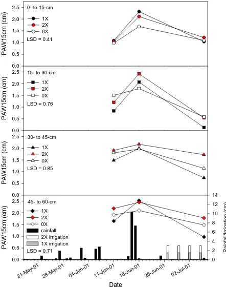
Effects of Sampling Date and Water Regime on Plant Available Water at Lewiston in 2001. ... 37
Plymouth 2001. ... 38
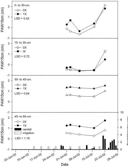
Lewiston 2002... 40
Plymouth 2002. ... 42
The Effect of Year and Location on Plant Available Water. ... 44
Location. ... 45
Year... 48
Water Regime. ... 49
Conclusion ... 51
Literature Cited ... 55
Chapter Three ... 72
Relationship Between Plant Available Water Measured Throughout the Growing Season and Yield... 72
Abstract... 73
Introduction... 74
Materials and Methods... 78
Results And Discussion ... 82
Location X Water Regime Interaction. ... 82
Year X Water Regime Interaction. ... 82
Water Regime Main Effect. ... 83
Effect of PAW15cm Measured at different Growth Stages on Corn Yield... 83
Conclusion ... 88
Literature Cited ... 91
Appendices... 113
Chapter Four ... 126
Relationship Between Plant Available Water Measured Throughout the Growing Season and Crop Water Stress ... 126
Abstract... 127
Introduction... 128
Materials and Methods... 132
Results and Discussion ... 137
Effects of Sampling Date and Water Regime by individual Site-Year ... 137
Analysis of Treatment Effects by Growth Stage. ... 141
Growth Stage Covariate Analysis... 143
Individual Location and Year Covariate Analysis... 143
Individual Measurement Date Covariate Analysis ... 144
Conclusion ... 147
Literature Cited ... 151
List of Tables
Table 2.1. Factors influencing PAW15cm at Lewiston 2001. ... 58
Table 2.2. Factors influencing PAW15cm at Plymouth 2001. ... 59
Table 2.3. Factors influencing PAW15cm at Lewiston 2002. ... 60
Table 2.4. Factors influencing PAW15cm at Plymouth 2002. ... 61
Table 2.5. Factors influencing PAW15cm at Growth Stage 1... 62
Table 2.6 . Factors influencing PAW15cm at Growth Stage 2... 63
Table 2.7. Factors influencing PAW15cm at Growth Stage 3... 64
Table 2.8. Factors influencing PAW15cm at Growth Stage 4... 65
Table 2.9. Factors influencing PAW15cm at Growth Stage 5... 66
Table 3.1. Effects of year, location and water regime on yield at Lewiston and Plymouth in 2001 and 2002... 94
Table 3.2. Effect of various factors on yield using PAW15cm as a covariate for different growth stages at 45- to 60-cm sampling depth at Lewiston and Plymouth in 2001 and 2002. Factors tested depending on data sets available at each stage. ... 95
Table 3.3. Effect of various factors on yield using PAW15cm as a covariate for different growth stages at 30- to 45-cm sampling depth at Lewiston and Plymouth in 2001 and 2002. Factors tested depending on data sets available at each stage. ... 96
Table 3.4. Maximum amount of PAW15cm at various sampling depths at Lewiston and Plymouth in 2001 and 2002. ... 97
Table 3.5. Lewiston 2001 correlation coefficients for relevance between PAW15cm and yield... 98
Table 3.6. Plymouth 2002 correlation coefficients for relevance between PAW15cm and yield... 99
Table 3.7. Analysis of the effects of water regime and PAW15cm as a covariate on CWSI on three dates at Plymouth in 2001... 100
Table 3.8. Analysis of the effects of water regime and PAW15cm as a covariate on CWSI on four dates at Plymouth in 2002 . ... 101
Table 4.1. Analysis of variance (ANOVA) of crop water stress index (CWSI) at each of four locations and years. ... 154
Table 4.2. Analysis of variance (ANOVA) of crop water stress index (CWSI) at each of five growth stages. ... 155
Table 4.3. Analysis of covariance (ANCOVA) of crop water stress index (CWSI) at growth stage IV with plant available water per fifteen centimeters of soil depth (PAW15cm) as a covariate. ... 156
Table 4.4. Overall correlation coefficients for relevance between PAW15cm (plant available water per fifteen centimeters of soil depth) and CWSI (crop water stress index) at five growth stages. ... 157
Table 4.6. Correlation coefficients for relevance between CWSI (crop water stress index) and PAW15cm (plant available water per fifteen centimeters of
soil depth) at four locations and years. ... 159 Table 4.7. Analysis of covariance (ANCOVA) of crop water stress index (CWSI)
on 17 July 2002 at Lewiston. ... 160 Table 4.8. Correlation coefficients for relevance between CWSI (crop water stress
index) and PAW15cm (plant available water per fifteen centimeters of
soil depth) on three measurement dates at Lewiston in 2002. ... 161 Table 4.9. Correlation coefficients for relevance between CWSI (crop water stress
index) and PAW15cm (plant available water per fifteen centimeters of
List of Figures
Figure 2.1. PAW15cm, measured rainfall, and estimated gated irrigation at
Lewiston in 2001. ... 67 Figure 2.2. PAW15cm, measured rainfall, and estimated gated irrigation at
Plymouth in 2001... 68 Figure 2.3. PAW15cm, measured rainfall, and estimated gated irrigation at
Lewiston in 2002. ... 69 Figure 2.4. PAW15cm, measured rainfall, and estimated gated irrigation at
Plymouth in 2002... 70 Figure 3.2. Differences in grain yield between 2001 and 2002 at the 0X, 1X and
2X irrigated treatments. Error bars represent LSD = 1.74 Mg ha-1. ... 103 Figure 3.3. Differences in grain yield across three water regimes. Error bars
represent LSD = 1.58 Mg ha-1. ... 104 Figure 3.4. The relationship between PAW15cm measured at four sampling depths
and grain yield at growth stage II. ... 105 Figure 3.5. The relationship between PAW15cm measured at four sampling depths
and grain yield at growth stage III. ... 106 Figure 3.6. The relationship between PAW15cm measured at four sampling depths
and grain yield at growth stage IV. ... 107 Figure 3.7. The relationship between PAW15cm measured at four sampling depths
and grain yield at Lewiston on 18 June 2001. ... 108 Figure 3.8. The relationship between PAW15cm measured at four sampling depths
and grain yield at Plymouth on 1 July 2002. ... 109 Figure 3.9. The relationship between PAW15cm measured at four sampling depths
and grain yield at Plymouth on 3 July 2002. ... 110 Figure 3.10. The relationship between PAW15cm measured at four sampling
depths and grain yield at Plymouth on 8 July 2002. ... 111 Figure 3.11. The relationship between PAW15cm measured at four sampling
depths and grain yield at Plymouth on 16 July 2002. ... 112 Figure 4.1. Linear regression of crop water stress index (CWSI) on plant available
water per fifteen centimeters of soil depth (PAW15cm) at the 0- to
15-cm sampling depth at growth stage IV. ... 163 Figure 4.2. Linear regression of crop water stress index (CWSI) on plant available
water per fifteen centimeters of soil depth (PAW15cm) at the 45- to 60-cm sampling depth at Lewiston in 2002. ... 164 Figure 4.3. Linear regression of crop water stress index (CWSI) on plant available
water per fifteen centimeters of soil depth (PAW15cm) at the 45- to 60-cm sampling depth at Lewiston on 17 July 2002. ... 165 Figure 4.4. Linear regression of crop water stress index (CWSI) on plant available
water per fifteen centimeters of soil depth (PAW15cm) at Lewiston on
9 July 2002. ... 166 Figure 4.5. Linear regression of crop water stress index (CWSI) on plant available
Chapter 1
Literature Review
Understanding and measuring the driving forces behind potential corn yield
within the growing season is vitally important. It allows adjustment of inputs to
maximize economic returns. Yield potential of corn is often impacted by limited
amounts of water, specifically the amount of available soil water (Roygard et al., 2002).
In the mid-Atlantic region, rainfall amounts during the growing season are usually
sufficient to produce profitable yields, but can be variable from year to year. Because
very little corn in Eastern North Carolina is irrigated, profitable production is heavily
dependent on the amount of rainfall and the soil’s ability to store water for plant growth.
Understanding the soil’s ability to hold water, how it varies over time, and quantifying
the relationship between water availability and yield are important steps that must be
taken to understand the yield potential of corn in the Mid-Atlantic Region. This project
was undertaken to understand the dynamics of water stored in the soil profile and its
influence on crop stress and yield.
Under ideal conditions for plant growth, a volume of soil generally
consists of 50% solids (mineral matter and organic matter), 25% air and 25% water
(Hillel, 1998). Soils, in terms of the ability to store water, can be described as a leaky
reservoir (Cassel and Nielson, 1986). A soil is considered to be at field capacity (FC)
when the “reservoir” is full. Field capacity, as defined in the Glossary of Soil Science
Terms (Soil Science Society of America, 1984), is the amount of water remaining in a
soil two to three days after having been wetted and after free drainage is negligible
(Cassel and Nielson, 1986). This corresponds with the generally accepted standard
soils, and -50 kPa for fine textured soils (Rivers and Shipp, 1977; Jamison and Kroth,
1958; Coleman, 1947). On the other hand, the permanent wilting point (PWP), defined
as the water content of a soil when indicator plants growing in that soil wilt and fail to
recover when placed in a humid chamber, is an indicator that the “reservoir” is dry.
Therefore, PWP represents the lower limit of the soil’s capacity to store water that can be
made available to plants. This corresponds with the generally accepted standard matric
potential of -1500 kPa for most soils. Except for some fine textured soils, the changes in
soil water content between pressures of -800 and -3000 kPa are negligible (McIntyre,
1974). The available water content (AWC) of a soil is defined as the difference between
FC and PWP and represents the potential plant extractable water that a soil can store
based on an indicator plant. Available water content can be expressed on the basis of
weight or volume.
To determine FC and PWP for a soil, a soil water retention analysis can be
performed in a lab on soil samples taken from the field, using a pressure plate apparatus
(Cassel and Nielson, 1986). This process establishes FC and PWP measurements for
each sample by applying the appropriate suction value and then measuring the
equilibrium soil wetness.
Methods of Measuring Soil Moisture. There are many direct and indirect methods to measure the amount of water stored in the soil (Gardner, 1986). The use of gravimetric
methods, electrical resistance, neutron scattering, and time-domain reflectometry (TDR)
method has advantages and disadvantages that limit the amount and kind of information
that can be obtained regarding soil moisture.
Methods for direct measurement of soil moisture include gravimetry with oven
drying (Gardner, 1986), which involves weighing a wet sample, removing the water by
oven drying the sample to a constant weight, and then reweighing the sample to
determine the amount of water removed. Dividing the difference between wet and dry
masses by the mass of the dry sample yields the ratio of the mass of water to the mass of
the dry soil, which when multiplied by 100, becomes the percentage of water in the
sample on a dry-weight basis. If a measure of volumetric water content is required, the
gravimetric water content is multiplied by the ratio of the soil bulk density to the density
of water.
Gravimetric methods are widely used because the samples can be easily taken,
they are inexpensive to conduct, and soil water content is easily calculated (Scott, 2000).
However, this method is both laborious and time consuming, and because of the
sampling, transporting, and repeated weighing procedures involved, contains many
opportunities for error (Hillel, 1998). The extraction of samples from the field is invasive
and destructive, potentially leading to distortion of experiments.
The most practical techniques for soil water monitoring are indirect methods
(Yoder et al., 1998; Robinson et al., 1999). Indirect techniques are divided into two
categories, tensiometric and volumetric methods, which estimate soil moisture content by
a calibrated relationship with some other measurable variable (Muñoz-Carpena, 2004).
Tensiometric methods include electrical resistance blocks, tensiometers, soil
Electrical resistance blocks, comprised of a pair of electrodes embedded in a
porous material such as gypsum (Bouyoucos and Mick, 1940) or fiberglass (Colman and
Hendrix, 1949) have been used because of their tendency to equilibrate with the matric
suction of soil water instead of the water content of the soil. The blocks operate on the
principle that the electrical resistance of a porous block is proportional to its water
content, which is related to the soil water matric potential of the surrounding soil
(Muñoz-Carpena, 2004). After being placed in the soil, the block reaches equilibrium, a
state in which soil water ceases to flow into or out of the block, and the electrical or
thermal properties of the block are then used as an index of soil water content. Soil water
content for the soil must be obtained by pressure plate extractor or gravimetric method
and then used to calibrate the block for accurate measurement. Use of electrical
resistance blocks are quick, repeatable, and relatively inexpensive, but sensitivity is poor
in dry soil conditions, and they do not work well in coarse-textured, high shrink-swell, or
saline soils. Block properties such as internal porosity change over time, depending on
the effect of soil type and rainfall on the degradation of gypsum. The time required to
attain equilibrium limits the accuracy of the measurements.
Tensiometers have been used for years to schedule irrigation of field and orchard
crops (Richards and Weaver, 1944). Tensiometers consist of a sealed water-filled tube
with a negative pressure gauge at one end and a ceramic cup at the other end which, when
placed in the soil, comes into equilibrium with the soil solution (Muñoz-Carpena, 2004).
The soil water matric potential is equivalent to the suction inside the tube. Soil water
content for the soil must be obtained independently by pressure plate extractor or
method allows for frequent and direct measurements of matric potential independent of
the use of electronic devices or a power source. Minimal skill is needed to read the
vacuum gauge, and the method is inexpensive to operate and maintain. Care must be
taken to ensure intimate contact between soil and the ceramic cup for consistent readings
in coarse textured soils. Response time is slow, and tubes must be refilled with water
frequently in hot, dry weather to maintain the water column inside the tensiometer.
Tensiometers have a narrow measurement range of less than 1 bar, restricting its use for
precise soil water measurements under extreme stress conditions.
Volumetric methods estimate the volume of water in a sample volume of
undisturbed soil (Muñoz-Carpena, 2004). Neutron probes can be used to measure
volumetric water content of soils (Gardner, 1970). Neutron probes were developed in the
1950’s, offering an efficient and reliable technique for measuring soil moisture in the
field (Holmes, 1956; van Bavel, 1963). Neutron probes are inserted into previously
prepared access holes in the soil which are lined with a metal casing (Muñoz-Carpena,
2004). The probe contains a sensor-detector with a decaying radioactive source emitting
fast neutrons that pass through the metal casing until being thermalized by hydrogen in
the soil and detected by the unit. Since water is the main source of hydrogen in most
soils, the density of thermalized neutrons around the probe is nearly proportional to the
volume of water contained in the soil. One probe can take measurements at any desired
depth, with a large sensing volume, but accuracy at depths within 0.20 m of the surface
are unreliable due to the escape of fast neutrons through the soil surface. While offering
repeatable measurements at the same locations and depths which were independent of
initial cost of the instrument are seen as disadvantages. Use of the neutron probe required
certification and the equipment is cumbersome and heavy. Soil specific calibration is
needed to utilize this technique.
The use of time domain reflectometry (TDR) has increased dramatically over the
last 30 years. Since the first application of TDR to measure soil water (Topp et al.,
1980), the use of the technology has been applied to measure soil electrical conductivity
as well. Based on the high dielectric constant of water, soil water content is inferred from
the dielectric permissivity of the soil (Jones et al., 2002). A step voltage pulse is
propagated along a transmission line (TDR probe) imbedded in the soil, and the length of
the propagation time is equated to soil percent moisture content. Unlike most other
techniques, soil specific calibration is usually not required (Muñoz-Carpena, 2004).
Measurements are highly accurate, and can be automated. A wide variety of probes are
commercially available, and probe installation can be achieved with minimal soil
disturbance. However, the equipment is relatively expensive, and the sensing volume of
the probe is relatively small.
A detailed investigation of the techniques described above indicates TDR as the
superior method to measure soil water content. Each technique has some characteristic
that is either equal or superior to TDR. However, no technique is superior to TDR in
more than one characteristic. Advantages of TDR over other soil water content
measurement methods are: (i) superior accuracy with minimal input; (ii) minimal
calibration requirements; (iii) no radiation hazard; (iv) excellent spatial and temporal
equipment to accommodate specific needs; and (vii) a non-destructive means of acquiring
measurements.
Factors Impacting Stored Soil Moisture. Soil moisture storage is impacted by soil texture, type of clay present, organic matter content, soil aggregation, and
evapotranspiration (Hillel, 1998). Loamy textured soils containing appreciable quantities
of silt usually hold the most plant available water (PAW), followed by clay, and then
sand. Clayey soils retain more water, and for a longer period of time, than do sandy soils.
These finer textured soils have a high specific surface, and therefore have a higher FC,
yet because the water is held so tightly, most of it is considered unavailable to the plant
resulting in a high PWP. Sandy soils have many large pores capable of quickly moving
water, hence good internal drainage but low storage capacity. The volume of small pores
in which water can be held is very small in sandy soils. Fine-textured clay soils have a
greater total volume of pores than coarse-textured sands, with the majority of those pores
being very small in size, so water does not move through quickly, and more water can be
stored. Some clays, such as montmorillonite, will shrink and crack when drying, which
provides for a high initial infiltration rate, and swell when wet, inhibiting infiltration.
Other clays, such as kaolinite, do not tend to shrink and swell.
The organic matter content (OMC) of a soil, if in sufficient quantities, can
enhance a soil’s ability to retain moisture by enhancing soil aggregation, resulting in
increased pore space. Soil organic matter physically and chemically binds the primary
particles in the aggregate which in turn increases the stability of the aggregate and limits
by soil organic matter. Soils with low aggregate stability are more susceptible to seal
formation as a result of raindrop impact, leading to lower infiltration rates
(Le Bissonnais, 1996). Hudson (1994) demonstrated that soils high in OMC store
significantly more water than soils of similar texture that contain less OMC, and that
these soils have more stored water available for plant growth.
The upward extraction of water from the soil surface and from plants by
evapotranspiration (ET) constantly impact the amount of water stored in the soil (Hillel,
1998). Evapotranspiration is the total amount of water lost from the field by both
evaporation and plant transpiration (Gardner et al., 1985). Evaporation is a direct
pathway for water to move from soil to the atmosphere as water vapor (Klockeet al.,
1996). Evaporation rates are highest after rainfall or irrigation, when the soil surface is
wet and water can evaporate readily and when the soil surface is not shaded. Evaporation
at this point is primarily influenced by the energy available for evaporation (Scott, 2000).
As the soil surface dries, the evaporation rate declines sharply, and is influenced mainly
by the hydraulic properties of the soil near the surface. Evaporation rates from the soil
surface also decline as the growing season progresses and canopy cover increases. At
this point, ET is comprised primarily of transpiration, defined as the process by which
water moves from the soil to the roots, from the roots into various parts of the plant, and
then into the leaves where it is released into the atmosphere as water vapor through the
stomata (Haman and Izuno, 1990). ET is measured as the atmospheric demand, or
potential ET (ETp), and as the crop’s ability to meet the atmospheric demand, actual ET
can be maximized. When ETa rates are significantly below ETp, soils are dryer, and
plants are under stress.
No-till and minimum-till management practices increase soil water holding
capacity by increasing soil aggregation and surface residues. No-till production methods
improve precipitation storage efficiency by maintaining more crop residue on the soil
surface (Smika, 1990). The residue moderates soil temperature by shading soil from
sunlight and increases soil water storage by enhancing precipitation infiltration (Smika
and Unger, 1986). Because soil aggregation is not adversely affected under no-till
systems, infiltration of rainfall or irrigation is enhanced, and evaporation losses are
minimized due to increased amounts of crop residue left on the soil surface (Brady,
1990). Tillage of the soil brings moist soil to the surface which increases soil water
evaporation compared to untilled soil (Burns et al., 1971; Papendick et al., 1973).
The temporal variation of soil moisture is influenced by several factors. At any
given point in time soil moisture (and thus PAW) is impacted by the precipitation history,
the texture of the soil, the slope of the terrain and presence of vegetation (Mohanty and
Skaggs, 2001). The dependency of the temporal stability of differences in soil water
storage on soil texture (see previous discussion on texture) was observed by Van Pelt and
Wierenga (2001). Temporal stability of soil moisture measurements is more stable
during dry periods, and less stable during the transition period between dry and wet soil
moisture status (Martínez-Fernández and Ceballos, 2003). Precipitation is the single
most important climatic factor for soil moisture and its distribution (Mohanty and
Skaggs, 2001). The presence of vegetation influences temporal soil moisture variability
Relationship Between PAW and Corn Yield. Researchers have concluded that climate (temperature and solar radiation) and water availability (soil water storage and rainfall)
are the major determining factors in corn production (Carlson, 1990; Dale and Daniels,
1995). Runge (1968) measured the influence of both maximum daily temperatures and
precipitation on corn yields and found that high temperatures were not detrimental if soil
moisture was not limiting. Yield of corn suffers in response to soil moisture deficits at
any growth stage (Howe and Rhoades, 1955). Eck (1984) found that stress imposed on
corn at the vegetative stages of growth for 14 and 28 days reduced yields by 23% and
46%, respectively. However, corn is especially sensitive to moisture stress during the
time of tasseling and continuing through grain fill (Musik and Dusek, 1980; Nesmith and
Ritchie, 1992). Denmead and Shaw (1960) reported that stress at vegetative growth
stages, at silking, and after silking reduced corn yield by 25%, 50%, and 21%,
respectively. Robins and Domingo (1953) found that corn yields were reduced by 22%
when soil moisture was reduced to wilting point for a period of 1 to 2 days during
tasseling or pollination, and that yields were reduced by 50% after 6 to 8 days of stress at
this stage. Musik and Dusek (1980) found soil moisture stress during periods of tasseling
and silking to be most detrimental to yield, and that soil moisture stress during the time of
grain fill was more harmful to yield than that during vegetative growth. Runge (1968)
and Thompson (1975) concluded that corn yield was highly correlated with water at
tasseling.
There is a need for research to understand within-season crop water use and how
seasonal crop water storage and yield. Holt et al. (1964) evaluated corn response to plant
available stored moisture at planting and found that yield was highly correlated to the
amount of stored soil moisture at planting during a year with below average rainfall.
Leeper et al. (1974) found that most of the corn yield variation within a field was
correlated with rooting depth, available water holding capacity in the root zone, or
weekly plant available stored soil moisture. Frye et al. (1983) reported that during years
of low rainfall, yield of corn was highly correlated to sampling depth. Swan et al. (1987)
observed that the effective plant rooting depth to corn yield relationships were influenced
significantly by climate, with higher correlations between yield and rooting depth during
years of low rainfall (Timlin et al., 1998). Roygard et al. (2002) compared yield across
three soil types of varying water-holding capacity at the vegetative, tasseling, and grain
filling stages of corn growth, and found that differences in water stress between soil types
were related to the capacity of the soils to store water. Schneider and Howell (1998)
compared the yields of corn across treatments in which soil water was maintained at five
levels in 25% increments ranging from 0 to 100% of AWC throughout the growing
season. They found that yields were highest when AWC of soils was held close to 100%
throughout the growing season.
Researchers have turned to plant growth models to maximize crop management
practices and predict yields (Xie et al., 2001). A general crop model called Agricultural
Land Management Alternatives with Numerical Assessment Criteria (ALMANAC) was
designed to simulate critical growth processes of a variety of crops (Kiniry et al., 1992).
Other models, such as CERES-Maize (Crop-Environment Resource Synthesis) (Jones
1989a) were designed for specific crop applications. These models predict crop yield by
incorporating numerous factors into daily estimates of crop growth and development
throughout the life cycle of the crop. One such factor is soil moisture. The effects of soil
moisture on crop growth and yield are determined by first calculating ETp and LAI (Leaf
Area Index), followed by the determination of a water stress factor based on soil water
supply and ETa which is used to estimate the decrease in daily crop growth and yield.
This water stress factor is a ratio of crop water use, based on PAW and rooting depth of
the crop, to crop water demand. If PAW in the current rooting zone is sufficient to meet
demand, yield is maximized. If PAW is restricted, then crop growth is restricted to that
amount of water. Factors influencing plant assimilation and leaf expansion growth are
calculated and applied to determine crop growth and yield predictions. Muchow et al.
(1994) used a sorghum growth simulation model to show that sorghum yields were
mainly associated with the amount of water stored in the soil at planting. Yields were
always higher where the soil water profile was full rather than half full at any planting
date and for any available soil water capacity at any location. Paz et al. (1998) used a
soybean model to correlate yield variability with variability of simulated water stress.
Moore and Tyndale-Brisco (1999), using crop models, observed that much of the
variability in wheat response to nitrogen could be explained by differing soil water
holding capacities.
Miller and Saunders (1923) reported the use of plant temperature as an indicator
of plant water status over 80 years ago. Research into the use of infrared thermometry to
remotely sense canopy temperature has continued since the early 1960s (Monteith and
the crop water stress index (CWSI) which was first defined and employed to measure
water stress in plants by Idso et al. (1981) and Jackson et al. (1981). Idso et al. (1981)
documented the linear relationship between the difference in canopy temperature and air
temperature (DT = Tc – Ta) and the vapor pressure deficit (VPD) of the air for well
watered plants transpiring at potential rate during daylight hours. This linear relationship
is sometimes called the “non water-stressed” or “lower” baseline, and it represents the
maximum rate of transpiration of a well watered, or non-stressed, crop. These lower
baselines are crop specific (Idso, 1982). Measurements of air temperature (Ta), canopy
temperature (Tc), relative humidity (RH), and wet bulb temperature (Tw) are taken
simultaneously to be used to construct the lower baselines needed for CWSI
determination. VPD is a measurement of the deficit between the amount of moisture in
the air at the time of measurement and the maximum amount of moisture the air can hold.
It can be calculated from measurements of RH, Ta, and Tw. To insure consistency, all
measurements were gathered following the procedures recommended by Gardner et al.
(1992).
As plants become stressed due to soil moisture depletion, the relationship between
DT and VPD deviates from that of the lower baseline condition. When soil moisture is
depleted this relationship is represented by the “water-stressed” or “upper” baseline. At
this level of stress, the baseline represents the DT of plants that are not transpiring, and
there is no response by Tc to VPD. Gardner and Shock (1989) found that multiplying the
original scale of 0 to 1 by 10 would yield a CWSI scale more easily understood and
accepted. On this scale, 0 indicated a crop under no stress and 10 indicated a crop under
Water stress in crops and CWSI have been related to soil water availability
(Hatfield,1983; Reginato and Garrot, 1987). Hatfield found that DT values for a well
watered crop of sorghum (Sorghum bicolor) remained negative, meaning leaf
temperatures were lower than air temperatures, until 65% of the PAW was extracted.
After 65% of the PAW was extracted, DT values became positive, meaning leaf
temperatures were higher than air temperatures, and increased quickly as PAW
decreased, indicating that the crop was under yield reducing stress. He also observed
that CWSI values summed over time provided a measure which is closely related to the
amount of PAW extracted from the soil. CWSI has also been used to schedule irrigation
for various crops including corn (Clawson and Blad, 1982; Neilsen and Gardner, 1987;
Yazar et al., 1999; Irmak et al., 2000) and to determine yield potential (Walker and
Hatfield, 1983; Irmak et al., 2000).
The purpose of this study is (i) to better understand the dynamic changes in PAW
under a crop of corn as the growing season progresses, and how these changes are
influenced by date, growth stage of corn, irrigation, and environment, (ii) to examine the
relationship of PAW measured at different growth stages and yield, and (iii) to determine
if there is a relationship between PAW and CWSI.
Literature Cited
Bouyoucos, G.J., and A.H. Mick. 1940. An electrical resistance method for the
continuous measurement of soil moisture under field conditions. Tech. Bull. 172. Michigan Agric. Exp. Stn., East Lansing.
Brady, N.C. 1990. The nature and properties of soils. 10th ed. Macmillan Publishing Comp. New York.
Burns, R.L., D.J. Cook, and R.E. Phillips. 1971. Influence of no tillage on soil moisture. Agron. J. 73:593-596.
Carlson, R.E. 1990. Heat stress, plant available soil moisture, and corn yields in Iowa: A short and long term view. J. Prod. Agric. 3:293-297.
Cassel, D.K., and D.R. Nielsen. 1986. Field capacity and available water capacity. p. 901–924. In A. Klute (ed.) Methods of soil analysis. Part 1. 2nd ed. Agron. Monogr. 9. ASA and SSSA, Madison, WI.
Clawson K.L., B.L. Blad. 1982. Infrared thermometry for scheduling irrigation of corn. Agron. J. 74:311-316.
Coleman, E.A. 1947. A laboratory procedure for determining the field capacity of soils. Soil Sci. 63:277-283.
Coleman E.A., and T.M. Hendrix. 1949. The fiberglass electrical soil-moisture instrument. Soil Sci. 67:425-438.
Dale, R.F., and J.A. Daniels. 1995. A weather-soil variable for estimating soil moisture stress and corn yield probabilities. Agron. J. 87:1115-1121.
Denmead, O.T., and R.H. Shaw. 1960. The effects of soil moisture stress at different stages of corn growth on the development and yield of corn. Agron. J. 52:272– 274.
Eck, H.V. 1986. Effects of water deficits on yield, yield components, and water use efficiency of irrigated corn. Agron. J. 78:1035–1040.
Emerson, W.W. 1977. Physical properties and structure. p. 78-104. In J.S. Russell and E.L. Greacen (ed.) Soil Factors in crop production in a semi-arid environment. Univ. of Queensland Press, St. Lucia, QLD, Australia.
Frye, W.W., C.W. Murdock, and R.L. Blevins. 1983. Corn yield-depth relationships on a Zanesville Soil. Soil Sci. Soc. Am. J. 47:1043-1045.
Gardner B.R., and C.C. Shock. 1989. Interpreting the crop water stress index. ASAE Paper 89-2642. ASAE, St. Joseph, MI.
Gardner B.R., D.C. Nielsen, and C.C. Shock. 1992. Infrared thermometry and the crop water stress index. II. Sampling procedures and interpretation. J. Prod. Agric. 5:466-475.
Gardner, F.P., R.B. Pearce, and R.L. Mitchell. 1985. Physiology of crop plants. Iowa State Univ. Press. Ames.
Gardner, W.H. 1986. Water content. p. 493–544. In A. Klute (ed.) Methods of soil analysis. Part 1. 2nd ed. Agron. Monogr. 9. ASA and SSSA, Madison, WI.
Gardner, W.R. 1970. Neutron meter use in soil moisture measurements. Isotopes and Radiation Tech. 7:297-305.
Halvorson, A.D., R.L. Anderson, S.E. Hinkle, D.C. Nielsen, R.A. Bowman, and M.F. Vigil. 1994. Alternative crop rotations to winter wheat-fallow. p. 6-11. In J.L. Havlin (ed.) Proc. Great Plains Soil Fertil. Conf., Vol. 5, Denver, CO. 7-8 Mar. 1994. Kansas State Univ., Manhattan.
Haman, D.Z., and F.T. Izuno. 1993. Soil plant water relationships. CIR1085. Florida Cooperative Extension Service, Institute of Food and Agricultural Sciences, University of Florida, Gainesville.
Hatfield, J.L. 1983. The utilization of thermal infrared radiation measurements from grain sorghum crops as a method of assessing their irrigation requirements. Irrig. Sci. 3:259-268.
Heiniger, R.W., J.F. Spears, D.T. Bowman, M.L. Carson, C.R. Crozier, E.J. Dunphy, S.R. Koenning, G.A. Payne, M.C. Marra, G.C. Naderman, J.W. Van Duyn, A.C. York, and A.S. Culpepper. 2002. Corn production guide. AG 590. N.C. Coop. Ext. Ser., N.C. State Univ., Raleigh.
Hillel, D. 1998. Environmental soil physics. Academic Press, New York.
Holmes, J.W. 1956. Calibration and field use of the neutron scattering method of measuring soil water content. Aust. J. Appl. Sci. 7:45-58.
Hudson, B.D. 1994. Soil organic matter and available water capacity. Journal of Soil and Water Conservation. 49(2):189-194.
Idso S.B., R.D. Jackson, P.J. Pinter, Jr., R.J. Reginato, and J.L. Hatfield. 1981.
Normalizing the stress-degree-day parameter for environmental variability. Agric. Meteorol. 24:45-55.
Irmak, S., D.Z. Hamman, and R. Bastug. 2000. Determination of crop water stress index for irrigation timing and yield estimation of corn. Agron. J. 92:1221–1227.
Jackson, R.D., S.B. Idso, R.J. Reginato, and P.J. Pinter, Jr. 1981. Canopy temperature as a crop water stress indicator. Water Resour. Res. 17:1133-1138.
Jamison, V.C., and E.M. Kroth. 1958. Available moisture storage capacity in relation to textural composition and organic matter content of several Missouri soils. Soil Sci. Soc. Am. Proc. 22:189-192.
Jones, C.A., and and J.R. Kiniry (ed.) 1986. CERES-Maize: A simulation model of maize growth and development. Texas A&M Univ. Press, College Station.
Jones, S.B., J.M. Wraith, and D. Or. 2002. Time domain reflectometry measurement principles and applications. Hydrol. Process. 16:141-153.
Kiniry, J.R., J.R. Williams, P.W. Gassman, and P. Debaeke. 1992. A general, process-oriented model for two competing plant species. Trans. ASAE 35:801-810.
Klocke, N.L., K.G. Hubbard, W.L. Kranz, and D.G. Watts. 1996. Evapotranspiration or crop water use [Online]. Available at http://ianrpubs.unl.edu/irrigation/g992.htm (verified 9 June 2005).
Leeper, R.A., E.C.A. Runge, and W.M. Walker. 1974. Effect of plant available stored soil moisture on corn yields. I. Constant climatic conditions. Agron. J. 66:723-727.
Le Bissonnais, Y. 1996. Aggregate stability and assessment of soil crusting and erodibility: 1. Theory and Methodology. Eur. J. Soil Sci. 47:425-437.
Martínez-Fernández, J., and A. Ceballos. 2003. Temporal stability of soil moisture in a large field experiment in Spain. Soil Sci. Soc. Am. J. 67:1647-1656.
McIntyre, D.S. 1974. Water retention and the moisture characteristic. p. 43-62. In J. Loveday (ed.) Methods for analysis of irrigated soils. Tech. Commun. Commonw. Bur. Soils no. 54. CAB: Fornham Royal, England.
Mohanty, B.P., and T.H. Skaggs. 2001. Spatio-temporal evolution and time-stable
characteristics of soil moisture within remote sensing footprints with varying soil, slope, and vegetation. Adv. Water Resour. 24:1051-1067.
Monteith, J.L., and G. Szeicz. 1962. Radiative temperature in the heat balance of natural surfaces. Q. J. R. Meteorol. Soc. 88:496-507.
Moore, G.A., and J.P. Tyndale-Brisco. 1999. Estimation of the importance of spatially variable nitrogen application and soil moisture holding capacity to wheat production. Prec. Agric. 1:27-38.
Muchow, R.C., G.L. Hammer, and R.L. Vanderlip. 1994. Assessing climatic risk to sorghum production in water-limited subtropical environments II. Effects of planting date, soil water at planting, and cultivar phenology. Field Crops Res. 36:235-246.
Muñoz-Carpena, R. 2004. Field devices for monitoring soil water content. Bull. 343. Florida Cooperative Extension Service, Institute of Food and Agricultural Sciences, University of Florida, Homestead.
Musick, J.T., and D.A. Dusek. 1980. Irrigated corn yield response to water. Trans. ASAE 23:92–103.
NeSmith, D.S., and J.T. Ritchie. 1992. Short- and long-term responses of corn to a pre-anthesis soil water deficit. Agron. J. 84:107–113.
Nielsen D.C., and B.R. Gardner. 1987. Scheduling irrigations for corn with the crop water stress index (CWSI). Appl. Agric. Res. 2:295-300.
Papendick, R.I., M.J. Lindstrom, and V.L. Cochran. 1973. Soil mulch effect on seedbed temperature and water during fallow in eastern Washington. Soil Sci. Soc. Am. Proc. 37:307-314.
Paz, J.O., W.D. Batchelor, T.S. Colvin, S.D. Logsdon, T.C. Kaspar, and D.L. Karlen. 1998. Analysis of water stress effects causing spatial yield variability in soybeans. Trans. ASAE 41:1527-1534.
Reginato, R.J., and D.J. Garrot, Jr. 1987. Irrigation scheduling with the crop water stress index. p. 7–10. In Western Cotton Production Conf. Summary Proc., Phoenix, AZ. 18–20 August, 1987. Cotton Growers Assoc., Memphis, TN.
Ritchie, S.W., J.J. Hanway, and G.O. Benson. 1993. How a corn plant develops. Spec. Rep. 48. Iowa State Univ., Ames.
Rivers, E.D., and R.F. Shipp. 1977. Soil water retention as related to particle size in selected sands and loamy sands. Soil Sci. 126:94-100.
Robins, J.S., and C.E. Domingo. 1953. Some effects of severe soil moisture deficits at specific growth stages in corn. Agron. J. 45:618–621.
Robinson, D.A., C.M.K. Gardner, and J.D. Cooper. 1999. Measurement of relative
permittivity in sandy soils using TDR, Capacitance, and Theta Probe: comparison, including the effect of bulk soil electrical conductivity. Journal of Hydrology. 223:198-211.
Rosenthal, W.D., R.L. Vanderlip, B.S. Jackson, and G.F. Arkin. 1989b. Sorkam: a grain sorghum crop growth model. Computer Software Documentation Ser. MP 1669. Texas Agric. Exp. Stn., College Station.
Roygard, J.K.F., M.M. Alley, and R. Khosla. 2002. No-till corn yields and water balance in the mid-Atlantic coastal plain. Agron. J. 94:612–622.
Runge, E.C. 1968. Effects of rainfall and temperature interactions during the growing season on corn yield. Agron. J. 60:503–507.
Sadler, E.J., P.J. Bauer, W.J. Busscher, and J.A. Millen. 2000. Site specific analysis of a droughted corn crop: II. Water use and stress. Agron. J. 92:403–410.
SAS Institute. 1998. SAS version 8.2. SAS Inst., Cary, NC.
Schneider, A.D., and T.A. Howell. 1998. LEPA and spray irrigation of corn—Southern High Plains. Trans. ASAE 41(5):1391–1396.
Scott, H.D. 2000. Soil Physics. Agricultural and environmental applications. Iowa State Univ. Press, Ames.
Smika, D.E. 1990. Fallow management practices for wheat production in the Central Great Plains. Agron. J. 82:319-323.
Smika, D.E., and P.W. Unger. 1986. Effect of surface residues on soil water storage. p. 111-138. In B.A. Stewart (ed.) Advances in soil science. Vol. 5. Springer-Verlag, New York.
SSSA. 1984. Gossary of soil science terms. Soil Science Society of America, Madison, WI.
Swan, J.B., M.J. Shaffer, W.H. Paulson, and A.E. Peterson. 1987. Simulating the effects of sampling depth and climatic factors on corn yield. Soil Sci. Soc. Am. J. 51:1025-1032.
Tanner, C.B. 1963. Plant temperatures. Agron. J. 55:210-211.
Thompson, L.M. 1975. Weather variability, climatic change, and grain production. Science 188:535–541.
Timlin, D.J., Y. Pachepsky, V.A. Snyder, and R.B. Bryant. 1998. Spatial and temporal variability of corn grain yield on a hillslope. Soil Sci. Soc. Am. J. 62:764-773.
Topp, G.C., J.L. Davis, and A.P. Annan. 1980. Electromagnetic determination of soil water content: Measurements in coaxial transmission lines. Water Resour. Res. 16:574–582.
Topp, G.C., S. Zegelin, and I. White. 2000. Impact of the real and imaginary components of relative permittivity on time domain reflectometry measurements in soils. Soil Sci. Soc. Am. J. 64:1244–1252.
U.S. Department of Agriculture. Natural Resource Conservation Service. 1981. Soil Survey of Washington County, North Carolina.
U.S. Department of Agriculture. Natural Resource Conservation Service. 1990. Soil Survey of Bertie County, North Carolina.
U.S. Department of Agriculture. Natural Resource Conservation Service. 1995. Soil Survey of Beaufort County, North Carolina.
Van Bavel, C.H.M. 1963. Neutron scattering measurement of soil moisture: Development and current status. Proc. Int. Symp. Humidity Moisture, p. 171-184, Washington, D.C.
Van Pelt, R.S., and P.J. Wierenga. 2001. Temporal stability of spatially measured soil matric potential probability density function. Soil Sci. Soc. Am. J. 65:668-677.
Walker G.K., and J.L. Hatfield. 1983. Stress measurement using foliage temperature. Agron. J. 75:623-629.
Yazar, A., T.A. Howell, D.A. Dusek, and K.S. Copeland. 1999. Evaluation of crop water stress index for LEPA irrigated corn. Irrig. Sci. 18:171-180.
Chapter Two
Abstract
Understanding and measuring the driving forces behind potential yield within the
growing season are vitally important in corn production. This knowledge allows
adjustment of inputs to maximize economic returns. The objective of this study is to
quantify the effects of location, year, and water regime on the dynamic temporal changes
in plant available water (PAW) over the growing season. Measurements of PAW were
taken over time at four sampling depths at Lewiston and Plymouth in 2001 and 2002.
Significant date x water regime interactions were measured at Plymouth at the upper two
sampling depths in 2001 and only at the 0- to 15-cm sampling depth in 2002. In 2002,
date was significant at the upper three sampling depths, and at Plymouth at the upper two
sampling depths only. Water regime was a significant factor on plant available water per
fifteen centimeters of soil depth (PAW15cm) only during the dry growing season in
2002. This study showed that rainfall, water treatments, and location (related to
differences in soil texture and how irrigation treatments were applied) were the main
factors influencing the dynamic changes in PAW measured at different sampling depths
in 2001 and 2002. Rainfall contributed heavily to changes in PAW at the shallow
sampling depths. The influence of irrigation was observed at the deeper sampling depths
due to the accumulation of water that was not affected by transpiration and evaporation.
Large changes in PAW occur at depths up to 30 cm, therefore it would be difficult to use
Introduction
Understanding and measuring the driving forces behind potential corn yield
within the growing season is vitally important since it allows adjustment of inputs to
maximize economic returns. Yield potential of corn is often impacted by limited
amounts of water, specifically the amount of available soil water (Roygard et al., 2002).
In the mid-Atlantic region, rainfall amounts during the growing season are usually
sufficient to produce profitable yields, but can be variable from year to year. Because
very little corn in this region is irrigated, profitable production is heavily dependent on
the amount of rainfall and the soils ability to store water for plant growth. Understanding
the dynamic temporal changes in plant available water (PAW) over the growing season is
vital if we are to quantify a relationship between PAW, crop water stress index (CWSI),
and yield potential of corn in the southeastern United States.
Field capacity (FC), as defined in the Glossary of Soil Science Terms (Soil
Sci. Soc. Am., 1984), is the amount of water remaining in a soil two to three days after
having been saturated and after free drainage is negligible (Cassel and Nielson, 1986).
This represents the maximum amount of water that the soil can store. In contrast, the
permanent wilting point (PWP) is defined as the water content of a soil when indicator
plants growing in that soil wilt and fail to recover when placed in a humid chamber.
Therefore, PWP represents the lower limit of the soil’s capacity to store water that can be
made available to plants. The available water content (AWC) of a soil is defined as the
difference between FC and PWP and represents the potential plant extractable water that
The amount of water stored in the soil at any given time is impacted by soil
texture, type of clay present, organic matter content, soil structure, tillage, and
evapotranspiration (Hillel, 1998). Loamy textured soils containing appreciable quantities
of silt usually hold the most PAW, followed by clay, and then sand. Clayey soils retain
more water, and for a longer period of time, than do sandy soils. These finer textured
soils have a high specific surface, and therefore have a higher FC, yet because the water
is held so tightly most water is unavailable to the plant, resulting in a high PWP. Sandy
soils have many large pores capable of quickly moving water, hence good internal
drainage but this results in a low storage capacity. The volume of small pores in which
water can be held is very small in sandy soils. Fine-textured clay soils have a greater
total volume of pores than coarse-textured sands, with the majority of those pores being
very small in size, so water does not move through quickly, and more water can be
stored. The organic matter content (OMC) of a soil, if in sufficient quantities, can
enhance a soils ability to retain moisture by enhancing soil aggregation, resulting in
increased pore space. Infiltration is also influenced by soil organic matter. Hudson
(1994) demonstrated that soils high in OMC store significantly more water than soils of
similar texture that contain less OMC, and that these soils have more of this stored water
available for plant growth.
The upward extraction of water from the soil surface and from plants by
evapotranspiration (ET) constantly impact the amount of water stored in the soil (Hillel,
1998). Evapotranspiration is the total amount of water lost from the soil by both
evaporation and plant transpiration (Gardner et al., 1985). Evaporation from soil is a
Evaporation rates are highest after rainfall or irrigation, when the soil surface is wet and
water can evaporate readily and when the soil surface is shaded. Evaporation at this point
is primarily influenced by the energy available for evaporation (Scott, 2000). As the soil
surface dries, the evaporation rate declines sharply, and is influenced mainly by the
hydraulic properties of the soil near the surface. Evaporation rates from the soil surface
also decline as the growing season progresses and canopy cover increases. At this point,
ET is comprised primarily of transpiration, defined as the process by which water moves
from the soil to the roots, from the roots into various parts of the plant, and finally into
the leaves where it is released into the atmosphere as water vapor through the stomata
(Haman and Izuno, 1990). ET is measured as the atmospheric demand, or potential ET
(ETp), and the crop’s ability to meet the atmospheric demand, actual ET (ETa). When
ETa rates are high, or close to ETp, soils are at or near FC and crop yield can be
maximized. When ETa rates are significantly below ETp, soils are dryer, and plants are
under stress.
No-till production methods improve water storage efficiency and soil water
availability (Halvorson et al., 1994). Tillage of the soil increases soil water evaporation
compared to untilled soil (Burns et al., 1971; Papendick et al., 1973). Because soil
aggregation is not adversely affected under no-till systems, infiltration of rainfall or
irrigation is enhanced, and evaporation losses are minimized due to increased amounts of
crop residue left on the soil surface (Brady, 1990).
There are many direct and indirect methods to measure the amount of water
stored in the soil (Gardner, 1986). The use of gravimetric methods, electrical resistance,
methods used to measure soil moisture (Hillel, 1998). One method for direct
measurement of soil moisture is gravimetry which involves the drying of soil in an oven
(Gardner, 1986). Gravimetric methods are widely used because the samples can be easily
taken, they are inexpensive to conduct, and soil water content is easily calculated (Scott,
2000). However, this method is both laborious and time consuming, and because of the
sampling, transporting, drying, and repeated weighing procedures involved; this method
presents many opportunities for error (Hillel, 1998). The extraction of samples from the
soil is invasive and destructive, potentially leading to distortion of experiments.
The most practical techniques for soil water monitoring are indirect methods
(Yoder et al., 1998; Robinson et al., 1999). Indirect techniques are divided into two
categories, tensiometric and volumetric methods. Both types estimate soil moisture
content by a calibrated relationship with some other measurable variable
(Muñoz-Carpena, 2004). Tensiometric methods include electrical resistance blocks and
tensiometers. Electrical resistance blocks have been used because of their tendency to
equilibrate with the matric suction of soil water instead of the water content of the soil.
Use of electrical resistance blocks are quick, repeatable, and relatively inexpensive, but
sensitivity is poor in dry soil conditions, and they do not work well in coarse-textured,
high shrink-swell, or saline soils. Soil water content for the soil must be obtained by
pressure plate extractor or gravimetric method and then used to calibrate the block for
accurate measurement. Block properties such as internal porosity change over time,
depending on the effect of soil type and rainfall on the degradation of gypsum, a
component of the blocks. The time required to attain equilibrium limits the accuracy of
Tensiometers have been used for years to schedule irrigation of field and orchard
crops (Richards and Weaver, 1944). This method allows for frequent and direct
measurements of matric potential, defined as the pressure potential of soil moisture
(Hillel, 1998). Matric potential results from the interactive capillary and adsorptive
forces between water and the soil matrix which bind water in the soil and lower it’s
potential energy below that of bulk water. Tensiometer readings can be taken without the
use of electronic devices or a power source. Minimal skill is needed to read the vacuum
gauge and the method is inexpensive to operate and maintain. Care must be taken to
ensure intimate contact between soil and the ceramic cup for consistent readings in coarse
textured soils. Like electrical resistance blocks, soil water content for the soil must be
obtained independently, by pressure plate extractor or gravimetric methods, to calibrate
tensiometer readings for soil water measurements. Response time is slow and tubes must
be refilled with water frequently in hot, dry weather to maintain the water column inside
the tensiometer. Tensiometers have a narrow measurement range of less than 1 bar,
restricting its use for precise soil water measurements under extremely dry conditions.
Volumetric methods include neutron probes and TDR. Neutron probes can be
used to measure volumetric water content of soils (Gardner, 1970). One probe can take
measurements at any desired depth, with a large sensing volume, but accuracy at depths
within 0.20 m of the surface are unreliable due to the escape of fast neutrons through the
soil surface. While offering repeatable measurements at the same locations and depths
which were independent of temperature and pressure, the health risk of exposure to
the neutron probe requires certification and the equipment is cumbersome and heavy.
Soil specific calibration is needed to utilize this technique.
The use of TDR has increased dramatically over the last 30 years. Unlike most
other techniques, soil specific calibration is usually not required (Muñoz-Carpena, 2004).
Measurements are highly accurate and can be automated. A wide variety of probes are
commercially available and probe installation can be achieved with minimal soil
disturbance. However, the equipment is relatively expensive and the sensing volume of
the probe is relatively small.
A detailed investigation of the techniques described above indicates TDR as the
superior method with which to measure soil water content for this project. Advantages of
TDR over other soil water content measurement methods are: (i) superior accuracy with
minimal input; (ii) minimal calibration requirements; (iii) no radiation hazard; (iv)
excellent spatial and temporal resolution; (v) easy to obtain measurements; (vi) a wide
array of commercially available equipment to accommodate specific needs; and (vii) a
non-destructive means of acquiring measurements.
The temporal variation of soil moisture is influenced by several factors. At any
given point in time soil moisture (and thus PAW) is impacted by the precipitation history,
the texture of the soil, the slope of the terrain and presence of vegetation (Mohanty and
Skaggs, 2001). In the Mid-Atlantic region, rainfall is known to vary temporally and
spatially (Roygard et al., 2002). Precipitation is the single most important climatic factor
for soil moisture and its distribution (Mohanty and Skaggs, 2001). The dependency of
the temporal stability of differences in soil water storage on soil texture (see previous
stability of soil moisture measurements is more stable during dry periods, and less stable
during the transition period between dry and wet soil moisture status
(Martínez-Fernández and Ceballos, 2003). The presence of vegetation influences temporal soil
moisture variability as it affects infiltration, runoff, and evapotranspiration. The
objective of this study is to quantify the effects of location, year, and water regime on the
Materials and Methods
Experiments were conducted at two locations in 2001 and 2002 at the Peanut Belt
Research Station (PBRS) at Lewiston, North Carolina and the Tidewater Research
Station (TRS) at Plymouth, North Carolina. At Lewiston in 2001, the predominate soil
types at the site were a Norfolk sandy loam (Fine-loamy, siliceous, thermic Typic
Paleudults) and a Goldsboro sandy loam (Fine-loamy, siliceous, thermic Aquic
Paleudults). At Plymouth in 2001, the experiment was conducted on a Portsmouth sandy
loam (Fine-loamy over sandy or sandy-skeletal, mixed, thermic Typic Umbraquults). In
2002, the soil types at Lewiston were Goldsboro and Lynchburg sandy loams
(Fine-loamy, siliceous, thermic Aeric Paleaquults), and a Rains sandy loam (Fine-(Fine-loamy,
siliceous, thermic Typic Paleaquults). Soils at the Plymouth site in 2002 were a
Portsmouth sandy loam and a Cape Fear loam (Clayey, mixed, thermic Typic
Umbraquults).
Fields were prepared and planted using conventional tillage methods. Row width
for both years at Lewiston was 91 cm and row width for both years at Plymouth was 96
cm. Pioneer 31G98 field corn was planted at a population of 67,500 seeds per hectare on
4 April 2001 and 6 April 2002 at Lewiston, and 30 April 2001 and 27 April 2002 at
Plymouth. Production practices were consistent with those generally used for profitable
corn production in eastern North Carolina. Weed control at both test sites in both years
was excellent due to proper timing and application of herbicides. Plots at Lewiston in
2001 received 168 kg 0-0-60 ha-1, 112 kg 0-46-0 ha-1, and 224 kg N ha-1 pre-plant, with
plots received 112 kg 0-0-60 ha-1 and 112 kg 18-46-0 ha-1 pre-plant, with 145 kg N ha-1
applied at growth stage V3. Plots at Plymouth in 2001 received 336 kg 9-23-30 ha-1
pre-plant and 224 kg N ha-1 applied at growth stage VT. In 2002, plots received 81 kg N ha-1
pre-plant and 49 kg N ha-1 applied at growth stage V3.
In 2001, the experimental design of the test was a modified Randomized
Complete Block with three water regimes as the main treatments replicated in three
blocks (Steel et al., 1997). Water regime treatments were comprised of no irrigation
(0X), normal irrigation (1X) and double irrigation (2X). At Lewiston, this was
accomplished using gated furrow irrigation by positioning the test on a slight grade with
the rows directed downhill and the 2X plots above the 1X plots. Alleys for each
treatment were flooded until water began to exit the far end of the plots. This system
worked well for providing two different levels of irrigation, but did not provide a way to
accurately measure the amount of water applied to each treatment. Irrigation in 1X plots
was estimated to be 1.5 cm and 2X plots received an estimated 3.0 cm per irrigation
(Barnes, 2004, personal communication). At Plymouth, plots were irrigated using an
overhead linear irrigation system which delivered 0.8 (1X) and 1.5cm (2X) of water per
irrigation. In 2002, the experimental design of the test was a modified Randomized
Complete Block with two water regimes (0X and 1X) as the main treatments, replicated
six times. Both locations were irrigated using overhead linear irrigation systems in 2002.
The system at Lewiston delivered an average of 1.4 cm of water at every event except
one, which measured 2.5 cm. The system at Plymouth applied 0.8 cm of water during
each irrigation. At both locations in both years, irrigations were scheduled when
Rainfall data used for this study was measured and recorded by personnel at TRS and
PBRS.
The goal for this study is to simultaneously take canopy temperature (discussed
later) and soil moisture measurements at least weekly at both locations. Canopy
temperature measurements require near cloudless conditions for an accurate measurement
to be made (Gardner et al., 1992). Measurements were taken on sunny days between
1100 hours and 1400 hours. In 2001, clear sunny days were rare. Uncooperative weather
for data collection allowed only three measurement dates at Lewiston and four
measurement dates at Plymouth. The same phenomena affected data collection in 2002
with only three measurement dates at Lewiston and five measurement dates at Plymouth.
Soil water content was measured using time domain reflectometry (TDR) probes
(MP-917, Environmental Sensors Inc., Victoria, BC, Canada) at 0- to 15-cm, 15- to
30-cm, 30- to 45-30-cm, and 45- to 60-cm sampling depths. After harvest, the probes were
removed and a 0.6-m deep hole was excavated to gather undisturbed samples from each
of the four sampling depths. A soil water retention analysis of the samples was
performed to determine PAW on a volume basis (Cassel and Nielson, 1986). Published
bulk density measurements for each soil (United States Department of Agriculture, 1981;
1990; 1995) were used for these calculations.
Grain yield was determined by harvesting the two center rows of each plot using a
Gleaner (AGCO Corp., Duluth, GA) two row combine. Moisture content and grain yield
were recorded using a HarvestMaster Grain Gauge (Juniper Systems, Inc., Logan, UT).
To understand the effect of sampling date on PAW15cm the data were separated
by location and year and analyzed using a split plot design with sampling date as the
main effect and water regimes as the sub-treatments. This resulted in the data being
separated into four groups: Lewiston 2001, Lewiston 2002, Plymouth 2001, and
Plymouth 2002. Each sampling depth at an individual location was tested for sampling
date and water regime main effects as well as sampling date X water regime interactions
using PROC GLM (SAS version 8.2, SAS Institute Inc, Cary, NC).
Planting dates differed across years and locations and it was impossible to
measure canopy temperatures and soil moisture at both locations on the same day.
Therefore, before examining the effects of location and year on PAW15cm, the data from
both years and locations were combined by crop growth stage to minimize the effects of
plant size and physiological development on the amount of PAW15cm present at
differing depths in the soil. Growing degree days (GDD) were calculated for each
measurement date and location, and the data was separated into as many identifiable
growth stages as possible. The data represented growth stages I (V15), II (V19/VT), III
(R1), IV (R2/R3), and V (R4) (Ritchie et al., 1993). All data collected for growth stage I
came from 19 June 2001 at Plymouth, so it was tested for water regime effects only using
PROC GLM (SAS version 8.2 SAS Institute Inc,, Cary, NC). Growth stage II included
data from both Plymouth and Lewiston in 2001, so it was tested for location and water
regime effects and a location X water regime interaction. Growth stages III and IV
included data collected at both locations and both years, so it was tested for location,
water regime, and year effects, as well as location X water regime and year X water
2002, so it was tested for location and water regime effects and location X water regime