INVESTIGATION
Study Designs for Identi
fi
cation of Rare Disease
Variants in Complex Diseases: The Utility of
Family-Based Designs
Iuliana Ionita-Laza*,1and Ruth Ottman†,‡
*Department of Biostatistics and†G. H. Sergievsky Center and Departments of Epidemiology and Neurology, Columbia University, New York, New York 10032, and‡Epidemiology Division, New York State Psychiatric Institute, New York, New York 10032
ABSTRACT The recent progress in sequencing technologies makes possible large-scale medical sequencing efforts to assess the importance of rare variants in complex diseases. The results of such efforts depend heavily on the use of efficient study designs and analytical methods. We introduce here a unified framework for association testing of rare variants in family-based designs or designs based on unselected affected individuals. This framework allows us to quantify the enrichment in rare disease variants in families containing multiple affected individuals and to investigate the optimal design of studies aiming to identify rare disease variants in complex traits. We show that for many complex diseases with small values for the overall sibling recurrence risk ratio, such as Alzheimer’s disease and most cancers, sequencing affected individuals with a positive family history of the disease can be extremely advantageous for identifying rare disease variants. In contrast, for complex diseases with large values of the sibling recurrence risk ratio, sequencing unselected affected individuals may be preferable.
C
OMMON diseases such as diabetes, cancer, and autism are likely caused by a complex interaction among many genes and environmental factors. Both common and rare genetic variants are expected to play a role. Thus far the available technology has allowed for the identification of common disease susceptibility variants, mostly via genome-wide association studies. However, the common variants de-tected so far have small effect sizes and overall explain only a small fraction of the estimated trait heritability (Maher 2008; Manolio et al. 2009). The recent advances in next-generation sequencing technologies (Metzker et al. 2010; Tucker et al. 2009) allow for the first time an objective assessment of the importance of rare variants in complex diseases. An increasing number of recent studies on hyper-tension, schizophrenia, epilepsy, type-1 diabetes, autism, etc. (Ji et al. 2008; Stefansson et al. 2008; Helbig et al.2009; Nejentsevet al.2009; Pintoet al.2010) implicate rare variants in these disorders.
Ongoing sequencing studies are already generating un-precedented amounts of genetic data. The large number of genetic variants in these data sets, most of them with low frequencies (,1%), creates great challenges for statistical analysis. Traditional association testing strategies that have worked well for common variants will have low power to identify rare disease susceptibility variants (Morris and Zeggini 2009; Bansal et al. 2010). To extract the rich in-formation provided by large sequencing data sets, several novel statistical approaches have been proposed, especially designed to identify rare variants that influence disease risk (Li and Leal 2008; Madsen and Browning 2009; Bhatiaet al.
2010; Han and Pan 2010; King et al. 2010; Liu and Leal 2010; Price et al. 2010; Ionita-Laza et al. 2011; Neale
et al.2011). The common idea underlying all these methods is to group variants in a region of interest,e.g., a gene, and perform a gene-based test rather than individual tests for each of the variants in a gene.
An important question that has not yet been addressed is the relative power of designs based on affected relativesvs.
designs using unselected affected individuals to identify rare disease variants. Since rare disease variants tend to be enriched in families containing multiple affected individuals, family-based designs can play an important role in the Copyright © 2011 by the Genetics Society of America
doi: 10.1534/genetics.111.131813
Manuscript received June 19, 2011; accepted for publication August 3, 2011 Supporting information is available online at http://www.genetics.org/content/ suppl/2011/08/12/genetics.111.131813.DC1.
1Corresponding author: 722 W. 168th St., 6th Floor, New York, NY 10025.
E-mail: [email protected]
identification of rare causal variants. The purpose of this article is to quantify this enrichment and to study its impli-cations for the optimal design of studies that search for rare disease variants in complex traits.
Methods
Effective number of variants in related individuals
By analogy to the concepts of“effective population size”in population genetics (Wright 1931, 1938) and “effective number of markers” in a linkage disequilibrium block (Nyholt 2004), we introduce here a new concept for analysis of rare variants in related individuals: theeffectivenumber of variants at a position, i.e., the number of “independent” variants at a specific position in a sample of related individ-uals. More precisely, the effective number of variants is the number of observed variantscorrectedfor the known familial correlation among the individuals included in a sample. This concept is important as it allows a uniform comparison of designs based on various types of relatives, regardless of the relationship type.
For simplicity of presentation we define the effective number of variants at a position for a pair of individuals. If the individuals are unrelated, then the effective number of variants is equal to the observed number of variants since the two individuals are independent (hence no correction is necessary). However, the effective number of variants in re-lated individuals is less than the total number of observed variants if some of the variants aresharedamong family mem-bers. For example, for a pair of siblings each of whom carries a rare variant in heterozygous state at a position, the effective number of variants will be less than the observed number of variants,i.e., two, due to the high probability that these two variants are shared identical-by-descent (IBD) and hence are not independent. Similarly, for a pair of second cousins that each carry a rare variant in heterozygous state the effective number of variants is less than two, although as shown in the examples below, it is higher than for a pair of siblings due to the lower likelihood that a variant is shared IBD for second cousins compared with siblings. Below we define mathemat-ically the concept of effective number of variants.
For a pair of relatives we define the effective number of variants, keff, as follows:
keff¼ 8 < :
keffj2 if both relatives carry a rare variant
keffj1 if only one of the two relatives carries a rare variant
keffj0 if neither of the two relatives carries a rare variant: By definition,keff|1= 1 andkeff|0= 0. Forkeff|2, we show in
supporting information, File S1that
keffj2ffilog2f h
4fuþ4f2124uþ4du2i; (1)
wherefis the frequency of the variant, anduis the kinship coefficient;d= 0 if the two relatives can share a maximum of one allele IBD (e.g.,first cousins) and 1 if they can share two alleles IBD (e.g., siblings). The approximation is based
only on the assumption that the variant is rare (i.e., f # 0.01) and is very accurate under this assumption.
When the two individuals are unrelated and each carries a rare variant,u= 0 and we obtain the expected result that
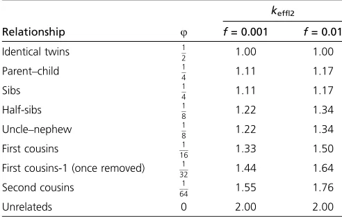
keff|2= 2. For identical twinsu= 0.5,d= 1, andkeff|2= 1.
For relatives in between, the effective number of variants is between 1 and 2. For two sibs,u¼14,d= 1, and hence for
f = 0.01 we obtainkeff|2 = 1.17. Similarly for two second
cousins,u¼ 1
64,d= 0, and hence keff|2= 1.76. These and
other examples are summarized in Table 1. Note that the effective number of variants depends on the frequency f. Hence, as expected, the lower the frequency is, the lower the effective number of variants, reflecting the low proba-bility that these shared variants are independent (and the greater chance they are identical-by-descent).
To summarize, for a pair of relativeskeffis calculated as
follows:
keff¼ 8 > > > > > > < > > > > > > :
log2f h
4fuþ4f2124uþ4
du2i
if both relatives carry a rare variant 1
if only one of the two relatives carries a rare variant 0
if neither of the two relatives carries a rare variant:
Under the assumption that the variant is not associated with disease, we calculate the expected value ofkefffor a pair
of relatives inFile S1(Equation S7) as
Ekeff
¼keffj24fð12fÞ
uþfð12fÞ124uþ4du2
þ keffj14fð12fÞ2
ð122uÞ2f124uþ4du2: (2)
At a rare variant position, for a data set of relative pairs of the same type in N different families, we define
kTotal eff ¼
PN
i¼1kieff, wherekieff is the effective number of
var-iants in familyi. Then
EhkTotaleff i¼NEkeff
: (3)
If the variant is not associated with disease, then the distribution of kTotal
eff can be approximated by a Poisson
distribution with mean¼E½kTotal
eff (as also shown
empiri-cally inFile S1,Figure S1)
Effective number of variants at a disease locus
At a disease locus, the effective number of variants in two affected relatives is expected to be increased compared to a nondisease locus. We consider here a two-locus genetic heterogeneity model (Risch 1990a), where each locus is an independent cause for disease. We use the two-locus model for mathematical convenience; without loss of gener-ality the second locus can be considered to encompass all the other disease loci that act additively to influence disease risk, in addition to the primary locus under investigation. The effective number of variants we expect to observe at thefirst disease locus in a pair of affected relatives is
EhkD eff
i
¼keffj24fð12fÞ
uþfð12fÞ124uþ4du2bR
þ keffj14fð12fÞ2
ð122uÞ2f124uþ4du2aR;
(4)
wherebR,aR$1 are derived inFile S1and depend on the
type of relationship R (e.g., sibs,first cousins, etc.), the ge-notype relative risk (GRR) for thefirst locus, and the overall recurrence risk in siblings as measured bylS(Risch 1990a).
The expression in Equation 4 is similar to the expression in Equation 2 for the effective number of variants expected at a nondisease locus. We performed simulations accord-ing to this model and show that the empirical estimates forE½kD
effagree very well with the analytical results in (4)
(see File S1).
For a data set ofNdifferent families, each consisting of an affected relative pair of the same type, we have
E h
kDeff;Total i
¼NE h
kDeff i
: (5)
As above, the distribution of kDeff;Totalcan be approximated
by a Poisson distribution with meanE½kDeff;Total(as also shown
empiricallyFile S1).
Furthermore, using Equation 4 we can also calculate the effective number of variants we expect at the first disease locus in an affected individualwithan affected relative. This is important to evaluate the importance of selecting affected individuals with a positive family history for a disease for inclusion in a sequencing study. We denote bykD
1 the number
of variants at thefirst locus in an affected individual that is known to have an affected relative. Then using Equation 4,
E h
kD1 i
¼14fð12fÞ uþfð12fÞ124uþ4du2bR
þ 0:54fð12fÞ2
ð122uÞ2f124uþ4du2aR;
where bR, aR $ 1 are derived in File S1. As above,
E½kD1;Total ¼NE½kD1for a data set of Naffected individuals,
each with an affected relative. Again it is true that
kD1;TotalPoissonðE½k D;Total 1 Þ.
Note that the description above pertains to a disease locus with only one disease variant position. However, a disease locus may have multiple disease variant positions (i.e., allelic heterogeneity). The extension to this scenario is straightforward by summing the effective number of var-iants at each position and using the fact that a sum of in-dependent Poisson random variables is also a Poisson random variable (we assume independence among the dif-ferent variant positions within a locus, a reasonable approx-imation given the low frequency of the variants).
Expected P-value at a disease locus
To compare the power of designs on the basis of biologically related casesvs.unrelated cases, we calculate an expectedP -value (EPV) (Dempster and Schatzoff 1965; Sackrowitz and Samuel-Cahn 1999). The expectedP-value, or expected sig-nificance level as originally defined in the pioneering article of Dempster and Schatzoff (1965), has been proposed as a measure of the performance of a test. Unlike the power of a test, the EPV does not depend on any prespecified sig-nificance level and is in close connection with the common practice of reportingP-values in applied research. The EPV is a single number that can be used to judge the performance of a test; the smaller the EPV is, the better the test.
For our situation, the effective number of variants under the null hypothesis that neither of the two loci is associated with disease, kTotal
eff , follows approximately a Poisson
distri-bution with mean l1 ¼E½kTotaleff as derived in Equation 3.
Similarly, the effective number of variants at thefirst disease locus in a two-locus disease model,kDeff;Total, follows approx-imately a Poisson distribution withl2¼E½kDeff;Totalas derived
in Equation 5. Then by definition the expectedP-value for thefirst disease locus is
EPV¼PðT1$T2Þ ¼PðT12T2$0Þ;
where T1 Poisson(l1) and T2 Poisson(l2). Since the
difference between two independent Poisson random varia-bles follows a Skellam distribution (Skellam 1946), we can calculate the EPV under a disease model only on the basis of the values ofl1andl2.
For comparison we also report results based on power, and, as shown below, they are highly correlated with those based on the EPV. Since we assume that the variant frequency in controls is known, the resulting power levels can be consid-ered as achievable as the number of controls grows very large.
Results
Performance of affected relatives vs. unrelated affected individuals
For identifying rare disease variants, it is of great interest to study the circumstances where study designs involving Table 1 The effective number of variants,keff|2, at a rare variant
position in two related individuals that each carry a variant, as defined in Equation 1
keff|2
Relationship u f= 0.001 f= 0.01
Identical twins 12 1.00 1.00 Parent–child 14 1.11 1.17
Sibs 14 1.11 1.17
Half-sibs 18 1.22 1.34
Uncle–nephew 18 1.22 1.34 First cousins 161 1.33 1.50 First cousins-1 (once removed) 1
32 1.44 1.64
Second cousins 1
64 1.55 1.76
Unrelateds 0 2.00 2.00
uis the kinship coefficient. Results for two values of the frequency parameterf, 0.001 and 0.01, are shown.
affected individuals from families containing multiple af-fected individuals are advantageous compared with those involving unselected affected individuals.
Under the assumption of a complex polygenic model, with many possible disease loci each with a small population attributable risk (Risch and Merikangas 1996), the two-locus disease model can be viewed as consisting of a two-locus of interest and a second locus accounting for the residual effect. We assume five study designs, each with the same number of affected individuals (i.e., 2000): affected sib-pairs, affected first-cousin pairs, affected second-cousin pairs, unrelated affected individuals, and unrelated affected individuals known to have an affected sibling. We consider a complex trait with prevalence 0.03 and a sibling recur-rence risk ratio (lS) between 2 and 10, as observed for many
complex traits (Merikangas and Risch 2003). We assume that the variant frequency at the first disease locus is low, between 0.0001 and 0.01, and several possible values for the genotype relative risk with higher GRRs are assumed for lower frequency at the disease locus. In Figure 1 we show expectedP-values associated with thefirst locus as a function of the sibling recurrence risk ratio, for each of thefive study designs.
For complex diseases with low values forlS(e.g., 2–4),
affected individuals known to have an affected sibling are
extremely advantageous to identify rare disease variants of moderate to large effect (e.g., GRR5–10, Figure 1). The difference between using affected individuals with an af-fected siblingvs.unselected affected individuals can be sub-stantial in this case. For example, for a disease withlS= 2,
for a locus with frequency 0.001 and a GRR of 5.5 the expectedP-value is 1027.65for a study with 2000 unrelated
affected individuals known to have an affected sibling and only 1023.77for a study with 2000 unselected affected
indi-viduals. Similarly, for a locus with frequency 0.0001 and a GRR of 14 the corresponding expectedP-values are 1027
and 10218. For small values ofl
Sand large values of GRR
(e.g.,lS= 2 and GRR = 14), even a design based on 1000
affected individuals known to have an affected sibling is expected to be more advantageous than a design based on 2000 unselected affected individuals (Figures 1 and 4). Sim-ilar results are obtained when the design comparison is based on power rather than expectedP-value (Figure S2).
However, for complex diseases with larger values of lS
such as autism (lS 22), the advantage of using
family-based designs (either affected relative pairs or affected indi-viduals with a known affected sibling) diminishes, and un-selected affected individuals can be more advantageous (Figure 2 and Figure S3). This trend of greater advantage with unselected affected individuals is more pronounced Figure 1 The effect of locus frequency, GRR, and overalllSon the relative performance (as measured by the expectedP-value) of affected relativesvs.
unrelated affected individuals. The three rows correspond to three different frequencies for the disease locus: 0.01, 0.001, and 0.0001.lSis between 2
and 10. The number of affected individuals is 2000: 1000 sib-pairs, 1000first-cousin pairs, 1000 second-cousin pairs, 2000 unrelateds, and 2000 unrelated individuals known to have an affected sibling (i.e., unrelateds+).
with increasing frequency of disease-causing variants (Fig-ure 1). These results are in concordance with those in Risch (1990b, 1992) for linkage analysis, which state that for small values of overalllSand polymorphic information
con-tent (PIC) (Botsteinet al. 1980) affected sib-pairs are opti-mal, while for large values of lS and PIC, more distantly
related individuals are best.
Above we have assumed that the disease locus has only one disease variant position. Although this is clearly a simplified scenario, the results obtained are informative for the more realistic scenario when the locus of interest contains multiple disease variants. In Figure 3 we show the results for the case when 5 different disease variant posi-tions are present at the locus. Two cases are illustrated: (1) the GRRs for the individual variants are a decreasing func-tion of frequency, so that lower-frequency variants have sub-stantially higher GRRs compared to more frequent variants (for example, f = 0.0001 and GRR = 21 vs. f = 0.01and GRR = 1.2), and (2) the GRR is the same for all variants (i.e., 2). As can be seen, for thefirst case, due to the pres-ence of high-risk low-frequency variants among the 5 dis-ease variants, unrelated affected individuals that are known to have an affected sibling are best for small values oflS(as
also shown previously in Figure 1), whereas for the second case where the GRR for low-frequency variants is modest (i.e., 2), distantly related affected individuals, and in partic-ular unselected affected individuals, perform better. Also shown are results when 10 additional random variants are added to the region. In this case, the relative performance of Figure 2 Usefulness of sequencing both affected individuals in a pair of
affected relatives. The three rows correspond to three different frequen-cies for the disease locus: 0.01, 0.001, and 0.0001. The number of af-fected individuals is 2000 for the two afaf-fected relatives design,i.e., 1000 sib-pairs and 1000 second-cousin pairs, and only 1000 for the design based on only one affected individual in a pair,i.e., 1000 affected indi-viduals known to have an affected sibling and 1000 affected indiindi-viduals known to have an affected second cousin.
Figure 3 Results are shown for scenarios where multiple (i.e., 5) disease susceptibility variants (DSVs) are present at the disease locus. The relationship between the GRR and disease variant frequency is shown in thefirst column. In the top panel, the GRR is a decreasing function of variant frequency, while in the bottom panel, the GRR is the same (i.e., 2) regardless of variant frequency. The third column presents results when 10 additional random variants (i.e., not disease variants) are also present.
different designs is unchanged, but the performance is re-duced for all designs.
The utility of sequencing both affected individuals in a pair of affected relatives
Sequencing both individuals from a pair of affected relatives doubles the sequencing costs, so it is important to consider the circumstances under which power is increased by this approach. We evaluated the utility of sequencing both affected individuals in an affected relative pair compared to sequencing only one individual from the pair (Figure 4 and Figure S4). We find that for affected sibling pairs, se-quencing the second sibling contributes little additional in-formation; hence sequencing only one of two affected siblings is expected to be on average almost as good as sequencing both of them, with the significant advantage of reducing the sequencing cost by half (Figure 4). However, for more dis-tantly related individuals, such as second cousins, sequencing both individuals is expected to be more powerful than se-quencing only one of them. The advantage can be significant. For example, whenlS= 2, for a locus with frequency 0.001
and a GRR of 5.5 the expected P-value is 1024for a study
with 1000 affected second-cousin pairs (power ata= 1.6· 1026is 87%) and only 1022.1for a study with 1000 affected
individuals known to have a second cousin affected (power is
47%). If instead we compare the power of a study with 1000 affected second-cousin pairs with that of a study with 2000 affected individuals known to have a second cousin affected, hence the same sequencing cost for both studies, wefind that the power levels are very similar (data not shown).
Discussion
In complex diseases characterized by extensive genetic heterogeneity, each disease locus is likely to be responsible for a very small fraction of affected individuals in a popula-tion. The choice of the affected individuals to be included in a study greatly influences the power to identify disease loci. The framework developed here, based on the effective number of variants in a pair of affected relatives, makes it feasible to quantify the enrichment in rare disease variants in family-based vs.population-based samples and to inves-tigate the optimal study design for identifying rare disease variants in complex traits.
We have shown here that for diseases with small values for the sibling recurrence risk ratio, as observed with many complex traits, sequencing affected individuals with an affected close relative, such as a sibling, can be an extremely powerful strategy for identifying rare disease variants with moderate to large GRRs. Thisfinding is in concordance with Figure 4 For complex traits with a large value forlS(e.g.,lS= 22 for autism) we show expectedP-values for a disease locus with frequencyf= 0.001 as
a function of the GRR forfive study designs, each with 2000 affected individuals: 1000 sib-pairs, 1000first-cousin pairs, 1000 second-cousin pairs, 2000 unrelateds, and 2000 unrelated individuals known to have an affected sibling (i.e., unrelateds+).
previous findings for breast cancer and common variants (Antoniou and Easton 2003). However, we find that the advantage of using affected individuals with a positive fam-ily history declines with increasing values oflS.For complex
diseases with large values oflS, such as autism (lS22),
unselected affected individuals may be preferable. The main explanation for these results is that for a complex disease involving many contributing disease loci, one single locus is likely to explain less of the overall familial aggregation when lSis large than when lSis small. Hence whenlSis large,
focusing on affected relatives (or individuals with an af-fected relative) may enrich the sample in rare disease loci that are less likely to be shared among multiple families, and therefore unselected affected individuals may be preferable. Designs based on affected relative pairs are commonly employed in linkage analysis (Weeks and Lange 1988). Al-though here we have not attempted to examine the perfor-mance of linkage analysis, we note that the results we obtained agree well with those for linkage analysis (Risch 1990b, 1992), which state that for small values of overalllS
and disease locus frequency affected sib-pairs are optimal, while for large values of lS and disease locus frequency,
more distantly related individuals are best.
The framework developed here is important for the statistical analysis of rare variant data. We have introduced here the concept of effective number of variants at a position in a set of relatives, which allows for a unified treatment of both biologically related and unrelated affected individuals and makes feasible natural extensions of statistical tests recently developed for population-based designs (such as the weighted-sum statistic in Madsen and Browning 2009) to general designs based on affected relative pairs and/or unrelated affected individuals. One simple statistic for af-fected relative pairs would be a weighted sum of the effective number of variants at different positions. Such extensions are currently under development.
The main goal of this article is to introduce a framework to assess the enrichment of rare disease mutations in affected relative pairs of different types. Such an enrichment analysis is of relevance for any association testing method, and therefore the results presented are expected to be valid in general for association testing. We have applied this framework to the problem of optimal study design for association studies with rare variants.
Software implementing the described methods is avail-able inFile S2, as well as on the first author’s webpage at
http://www.columbia.edu/~ii2135/, and should be helpful in the design of association studies with rare variants.
Acknowledgments
We are grateful to Mitchell Gail and Joseph Buxbaum for useful discussions. We also thank the associate editor and two reviewers for their comments that helped improve our article. This work was supported by grants R03HG005908-2 (to I.I.-L.) and RC2 NS070344 (to R.O.) from the National
Institutes of Health and DMS-1100279 (to I.I.-L.) from the National Science Foundation.
Literature Cited
Antoniou, A. C., and D. F. Easton, 2003 Polygenic inheritance of
breast cancer: implications for design of association studies.
Genet. Epidemiol. 25: 190–202.
Bansal, V., O. Libiger, A. Torkamani, and N. J. Schork,
2010 Statistical analysis strategies for association studies
in-volving rare variants. Nat. Rev. Genet. 11: 773–785.
Bhatia, G., V. Bansal, O. Harismendy, N. J. Schork, E. J. Topolet al.,
2010 A covering method for detecting genetic associations
be-tween rare variants and common phenotypes. PLoS Comput. Biol. 6: e1000954.
Botstein, D., R. L. White, M. Skolnick, and R. W. Davis,
1980 Construction of a genetic linkage map in man using
re-striction fragment length polymorphisms. Am. J. Hum. Genet.
32: 314–331.
Dempster, A. P., and M. Schatzoff, 1965 Expected significance
level as a sensitivity index for test statistics. J. Am. Stat. Assoc.
60: 420–436.
Han, F., and W. Pan, 2010 A data-adaptive sum test for disease
association with multiple common or rare variants. Hum. Hered.
70: 42–54.
Helbig, I., H. C. Mefford, A. J. Sharp, M. Guipponi, M. Ficheraet al.,
2009 15q13.3 microdeletions increase risk of idiopathic
gen-eralized epilepsy. Nat. Genet. 41: 160–162.
Ionita-Laza, I., J. Buxbaum, N. M. Laird, and C. Lange, 2011 A
new testing strategy to identify rare variants with either risk or protective effect on disease. PLoS Genet. 7: e1001289.
Ji, W., J. N. Foo, B. J. O’Roak, H. Zhao, M. G. Larson et al.,
2008 Rare independent mutations in renal salt handling genes
contribute to blood pressure variation. Nat. Genet. 40: 592–599.
King, C. R., P. J. Rathouz, and D. L. Nicolae, 2010 An evolutionary
framework for association testing in resequencing studies. PLoS Genet. 6: e1001202.
Li, B., and S. M. Leal, 2008 Methods for detecting associations
with rare variants for common diseases: application to analysis
of sequence data. Am. J. Hum. Genet. 83: 311–321.
Liu, D. J., and S. M. Leal, 2010 A novel adaptive method for the
analysis of next-generation sequencing data to detect complex trait associations with rare variants due to gene main effects and interactions. PLoS Genet. 6(10): e1001156.
Madsen, B. E., and S. R. Browning, 2009 A groupwise association
test for rare mutations using a weighted sum statistic. PLoS Genet. 5: e1000384.
Maher, B., 2008 Personal genomes: the case of the missing
heri-tability. Nature 456: 18–21.
Manolio, T. A., F. S. Collins, N. J. Cox, D. B. Goldstein, L. A.
Hindorffet al., 2009 Finding the missing heritability of
com-plex diseases. Nature 461: 747–753.
Merikangas, K. R., and N. Risch, 2003 Genomic priorities and
public health. Science 302: 599–601.
Metzker, M. L., 2010 Sequencing technologies—the next
genera-tion. Nat. Rev. Genet. 11: 31–46.
Morris, A. P., and E. Zeggini, 2009 An evaluation of statistical
approaches to rare variant analysis in genetic association
stud-ies. Genet. Epidemiol. 34: 188–193.
Neale, B. M., M. A. Rivas, B. F. Voight, D. Altshuler, B. Devlinet al.,
2011 Testing for an unusual distribution of rare variants. PLoS
Genet. 7: e1001322.
Nejentsev, S., N. Walker, D. Riches, M. Egholm, and J. A. Todd,
2009 Rare variants of IFIH1, a gene implicated in antiviral
responses, protect against type 1 diabetes. Science 324: 387–
389.
Nyholt, D. R., 2004 A simple correction for multiple testing for single-nucleotide polymorphisms in linkage disequilibrium with
each other. Am. J. Hum. Genet. 74: 765–769.
Pinto, D., A. T. Pagnamenta, L. Klei, R. Anney, D. Merico et al.,
2010 Functional impact of global rare copy number variation
in autism spectrum disorders. Nature 466: 368–372.
Price, A. L., G. V. Kryukov, P. I. de Bakker, S. M. Purcell, J. Staples
et al., 2010 Pooled association tests for rare variants in
exon-resequencing studies. Am. J. Hum. Genet. 86: 832–838.
Risch, N., 1990a Linkage strategies for genetically complex traits.
I. Multilocus models. Am. J. Hum. Genet. 46: 222–228.
Risch, N., 1990b Linkage strategies for genetically complex traits.
III. The effect of marker polymorphism on analysis of affected
relative pairs. Am. J. Hum. Genet. 46: 242–253.
Risch, N., 1992 Corrections to“Linkage strategies for genetically
complex traits. III. The effect of marker polymorphism on
anal-ysis of affected relative pairs”. Am. J. Hum. Genet. 51: 673–675.
Risch, N., and K. Merikangas, 1996 The future of genetic studies
of complex human diseases. Science 273: 1516–1517.
Sackrowitz, H. B., and E. Samuel-Cahn, 1999 P-values as random
variables: expected P-values. Am. Stat. 53: 326–331.
Skellam, J. G. 1946 The frequency distribution of the difference
between two Poisson variates belonging to different popula-tions. J. R. Stat. Soc. Ser. A, 109: 296.
Stefansson, H., D Rujescu, S Cichon, O. P Pietilinen, A Ingason
et al., 2008 Large recurrent microdeletions associated with
schizophrenia. Nature 455: 232–236.
Tucker, T., M. Marra, and J. M. Friedman, 2009 Massively parallel
sequencing: the next big thing in genetic medicine. Am. J. Hum.
Genet. 85: 142–154.
Weeks, D. E., and K. Lange, 1988 The affected-pedigree-member
method of linkage analysis. Am. J. Hum. Genet. 42: 315–326.
Wright, S., 1931 Evolution in Mendelian populations. Genetics
16: 97–159.
Wright, S., 1938 Size of population and breeding structure in
re-lation to evolution. Science 87: 430–431.
Communicating editor: S. F. Chenoweth
GENETICS
Supporting Information
http://www.genetics.org/content/suppl/2011/08/12/genetics.111.131813.DC1
Study Designs for Identi
fi
cation of Rare Disease
Variants in Complex Diseases: The Utility of
Family-Based Designs
Iuliana Ionita-Laza and Ruth Ottman
Supplemental Material
S1
Effective number of variants in related individuals
We derive here in detail the results in the text, in particular relations (1) and (2).
Assumption S1.
We assume for simplicity that all individuals who carry a rare variant
are in fact heterozygous. This assumption is reasonable for our setting since homozygous
genotypes would have very low probability for rare variants (
f
2≤
10
−4for
f
≤
0
.
01
).
We are interested in computing the joint distribution of the genotypes at a position in
two related individuals. Let us code the genotype of an individual as 0, 1 or 2, denoting
the number of rare variants (or minor alleles) in the genotype. For example, a homozygous
genotype for the rare variant is denoted by 2 (however, we ignore individuals with genotype
2 by Assumption S1).
Claim S2.
Let
p
{i,j}be the probability that the genotypes in two related individuals are
i
and
j
, with
i, j
∈ {
0
,
1
}
. Let
ϕ
be the kinship coefficient for the two relatives,
f
be the minor
allele frequency at a variant position, and
δ
be
1
if the two relatives can share two alleles
IBD, and
0
if the two relatives can share a maximum of one allele IBD. Then the following
relationships are true:
p{0,0} (1−f)2·[1−2f(1−2ϕ) +f2(1−4ϕ+ 4δϕ2)] p{0,1} 4f(1−f)2·[(1−2ϕ)−f(1−4ϕ+ 4δϕ2)] p{1,1} 4f(1−f)·[ϕ+f(1−f)(1−4ϕ+ 4δϕ2)]
Table S-1: Joint probabilities for the genotypes in two related individuals.
Proof.
To calculate
p
{i,j}we condition on the IBD sharing between the two individuals.
There are at most two alleles that can be shared IBD between two individuals, depending
on the precise relationship. Let
p
ij|kbe the probability that in a set of relatives the first
genotype is
i
and the second genotype is
j
conditional on the IBD sharing being
k
, where
i, j
∈ {
0
,
1
}
and 0
≤
k
≤
2. We now calculate the probabilities
p
ij|kin turn.
- IBD sharing is 0 with probability
P
(
IBD
= 0) = 1
−
4
ϕ
+ 4
δϕ
2.
Because the genotypes at the two relatives are independent in this case it is relatively
easy to calculate
p
ij|0(Table S-2).
The results in the table are based on multiplying the probabilities of individual
geno-types. For example,
p
01|0=
P
(genotype 1 is 0 and genotype 2 is 1
|
IBD
= 0) = (1
−
f
)
2·
2
f
(1
−
f
) = 2
f
(1
−
f
)
3.
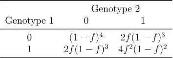
21
Genotype 2 Genotype 1 0 1
0 (1−f)4 2f(1−f)3 1 2f(1−f)3 4f2(1−f)2
Table S-2: Joint probabilities for the genotypes in two related individuals, conditional on
the IBD sharing being 0, i.e.,
p
ij|0.
- IBD sharing is 1 with probability
P
(
IBD
= 1) = 4
ϕ
−
8
δϕ
2.
Results for
p
ij|1are in Table S-3.
Genotype 2 Genotype 1 0 1
0 (1−f)3 f(1−f)2 1 f(1−f)2 f(1−f)
Table S-3: Joint probabilities for the genotypes in two related individuals, conditional on
the IBD sharing being 1, i.e.,
p
ij|1.
The results in the table are calculated as follows:
p
00|1=
P
(genotype 1 is 0 and genotype 2 is 0
|
IBD
= 1) =
=
P
(genotype 1 is 0
|
genotype 2 is 0 and
IBD
= 1)
P
( genotype 2 is 0
|
IBD
= 1) =
= (1
−
f
)
·
(1
−
f
)
2= (1
−
f
)
3.
Also
p
10|1=
P
(genotype 1 is 1 and genotype 2 is 0
|
IBD
= 1) =
=
P
(genotype 1 is 1
|
genotype 2 is 0 and
IBD
= 1)
P
( genotype 2 is 0
|
IBD
= 1) =
=
f
·
(1
−
f
)
2.
Similarly
p
11|1=
P
(genotype 1 is 1 and genotype 2 is 1
|
IBD
= 1) =
=
P
(genotype 1 is 1
|
genotype 2 is 1 and
IBD
= 1)
P
( genotype 2 is 1
|
IBD
= 1) =
=
1
2
f
+
1
2
(1
−
f
)
·
2
f
(1
−
f
) =
f
(1
−
f
)
.
22
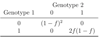
Genotype 2 Genotype 1 0 1
0 (1−f)2 0 1 0 2f(1−f)
Table S-4: Joint probabilities for the genotypes in two related individuals, conditional on
the IBD sharing being 2, i.e.,
p
ij|2.
- IBD sharing is 2 with probability
P
(
IBD
= 2) = 4
δϕ
2.
In this case, the two genotypes are identical. Results for
p
ij|2are in Table S-4.
It is relatively easy to derive the results in the table. For example:
p
11|2=
P
(genotype 1 is 1 and genotype 2 is 1
|
IBD
= 2) =
=
P
(genotype 1 is 1
|
genotype 2 is 1 and
IBD
= 2)
P
(genotype 2 is 1
|
IBD
= 2) =
= 1
·
2
f
(1
−
f
) = 2
f
(1
−
f
)
.
From Tables S-2, S-3 and S-4 we get:
p
{0,0}=
P
(genotype 1 is 0 and genotype 2 is 0) =
=
p
00|0P
(
IBD
= 0) +
p
00|1P
(
IBD
= 1) +
p
00|2P
(
IBD
= 2)
= (1
−
f
)
2·
[(1
−
4
ϕ
+ 4
δϕ
2)(1
−
f
)
2+ (4
ϕ
−
8
δϕ
2)(1
−
f
) + 4
δϕ
2]
.
(S3)
p
{0,1}=
P
(genotype 1 is 0 and genotype 2 is 1
OR
genotype 1 is 1 and genotype 2 is 0) =
= 2
P
(genotype 1 is 0 and genotype 2 is 1) =
= 2(
p
01|0P
(
IBD
= 0) +
p
01|1P
(
IBD
= 1) +
p
01|2P
(
IBD
= 2))
= 2
f
(1
−
f
)
2·
[2(1
−
4
ϕ
+ 4
δϕ
2)(1
−
f
) + (4
ϕ
−
8
δϕ
2)]
.
(S4)
p
{1,1}=
P
(genotype 1 is 1 and genotype 2 is 1) =
= 2(
p
11|0P
(
IBD
= 0) +
p
11|1P
(
IBD
= 1) +
p
11|2P
(
IBD
= 2))
=
f
(1
−
f
)
·
[4(1
−
4
ϕ
+ 4
δϕ
2)
f
(1
−
f
) + (4
ϕ
−
8
δϕ
2) + 8
δϕ
2]
.
(S5)
Using simple algebraic manipulation it is possible to simplify the above expressions for
p
{0,0},
p
{0,1}, and
p
{1,1}(Table S-5).
We can easily check the two extreme cases:
ϕ
= 0,
δ
= 0 (unrelated individuals, Table
S-6) and
ϕ
= 0
.
5,
δ
= 1 (identical twins, Table S-7).
p{0,0} (1−f)2·[1−2f(1−2ϕ) +f2(1−4ϕ+ 4δϕ2)]
p{0,1} 4f(1−f)2·[(1−2ϕ)−f(1−4ϕ+ 4δϕ2)] p{1,1} 4f(1−f)·[ϕ+f(1−f)(1−4ϕ+ 4δϕ2)]
Table S-5: Joint probabilities
p
{i,j}for the genotypes in two related individuals.
p{0,0} (1−f)2(1−f)2
p{0,1} (1−f)2·2f(1−f) + 2f(1−f)·(1−f)2 p{1,1} [2f(1−f)]·[2f(1−f)]
Table S-6: Joint probabilities for the genotypes in two unrelated individuals (
ϕ
= 0,
δ
= 0).
p{0,0} (1−f)2 p{0,1} 0 p{1,1} 2f(1−f)
Table S-7: Joint probabilities for the genotypes in two identical twins (
ϕ
= 0
.
5,
δ
= 1).
Claim S6.
For a pair of individuals that each carry a rare variant in heterozygous state we
calculate the effective number of variants for the pair as:
k
eff|2∼
= log
2f[4
fϕ
+ 4
f
2(1
−
4
ϕ
+ 4
δϕ
2)]
.
Proof.
We define the
effective
number of variants in a pair of individuals that are both
heterozygous, denoted by
k
eff|2, to satisfy the equation:
P
(genotype 1 is 1 and genotype 2 is 1
|
neither genotype is 2) =
=
P
(genotype 1 is 1
|
genotype 1 is not 2)
keff|2.
When the two individuals are unrelated we can see that
k
eff|2should be 2. Similarly, when
the two individuals are identical twins
k
eff|2should be 1, as expected.
In order to define
k
eff|2we need to calculate first the probability that two relatives are both
heterozygous, given that they are not homozygous (as by Assumption S1). More precisely,
for a pair of relatives we have:
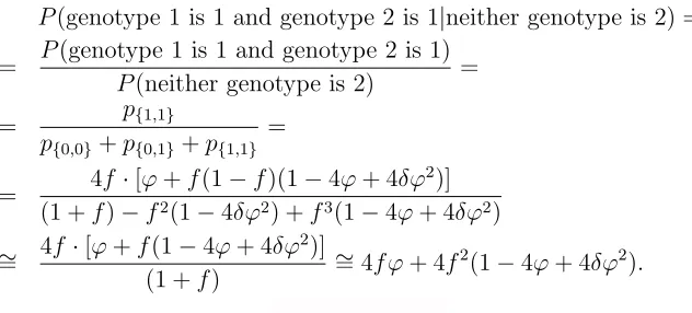
P
(genotype 1 is 1 and genotype 2 is 1
|
neither genotype is 2) =
=
P
(genotype 1 is 1 and genotype 2 is 1)
P
(neither genotype is 2)
=
=
p
{1,1}p
{0,0}+
p
{0,1}+
p
{1,1}=
=
4
f
·
[
ϕ
+
f
(1
−
f
)(1
−
4
ϕ
+ 4
δϕ
2
)]
(1 +
f
)
−
f
2(1
−
4
δϕ
2) +
f
3(1
−
4
ϕ
+ 4
δϕ
2)
∼
=
4
f
·
[
ϕ
+
f
(1
−
4
ϕ
+ 4
δϕ
2
)]
(1 +
f
)
∼
= 4
fϕ
+ 4
f
2
(1
−
4
ϕ
+ 4
δϕ
2)
.
24
In the approximation above, we approximate
f
(1
−
f
)
∼
=
f
and (1 +
f
)
−
f
2(1
−
4
δϕ
2) +
f
3(1
−
4
ϕ
+ 4
δϕ
2)
∼
= 1 for
f
≤
0
.
01. These approximations are very good, and have only
negligible effect.
Also the probability that an individual is heterozygous, conditional on not being
homozy-gous is:
P
( genotype is 1
|
genotype is not 2) =
2
f
(1
−
f
)
1
−
f
2=
2
f
1 +
f
∼
= 2
f
if we assume that 1 +
f
∼
= 1 for
f
≤
0
.
01. As can be seen, the conditioning on the genotype
not being 2 has negligible effect, so we will ignore it in subsequent calculations.
By definition the
effective
number of variants in a pair of individuals that are both
heterozygous, denoted by
k
eff|2, satisfies the equation:
P
(genotype 1 is 1 and genotype 2 is 1
|
neither genotype is 2) =
=
P
(genotype 1 is 1
|
genotype 1 is not 2)
keff|2.
Using the relationships above we get:
k
eff|2∼
= log
2f[4
fϕ
+ 4
f
2(1
−
4
ϕ
+ 4
δϕ
2)]
.
Note that the above approximation is extremely good. It is easy to see that for two
unre-lated individuals, since
ϕ
= 0 and
δ
= 0, we get
k
eff|2= 2; for two identical twins, since
ϕ
= 0
.
5 and
δ
= 1 we get
k
eff|2= 1. These values match our intuition, namely, that for
unrelated individuals the two variants are indepedent, while for identical twins there is only
one independent variant.
If only one of the two relatives carries a rare variant, then the
effective
number of variants
in the pair, denoted by
k
eff|1, is 1. Similarly, if neither of the two relatives is carrier of rare
variant, then
k
eff|0= 0. For a pair of relatives we calculate the
effective
number of variants,
denoted by
k
eff, as follows:
k
eff=
⎧
⎨
⎩
k
eff|2if both relatives carry a rare variant
k
eff|1if only one of the two relatives carries a rare variant
k
eff|0if neither of the two relatives carries a rare variant
Using the derivations above, we can now calculate the
effective
number of variants
ex-pected at a variant position in a pair of individuals:
E
[
k
eff] =
k
eff|2p
{1,1}+
k
eff|1p
{1,0}=
=
k
eff|2·
4
f
(1
−
f
)
·
[
ϕ
+
f
(1
−
f
)(1
−
4
ϕ
+ 4
δϕ
2)] +
+
k
eff|14
f
(1
−
f
)
2·
[(1
−
2
ϕ
)
−
f
(1
−
4
ϕ
+ 4
δϕ
2)]
.
(S7)
25
S2
Effective number of variants in affected relatives at a
disease
locus
In a similar fashion, we can also calculate the
effective
number of variants we expect to
observe at a
disease
locus, and derive relation (4) in text. We assume a two-locus genetic
heterogeneity model, with either locus being an independent disease cause. Similar to the
derivations above we calculate
p
D{i,j}, i.e., the probability that two affected relatives have
genotypes
i
and
j
at the first disease locus, with
i, j
∈ {
0
,
1
}
. Using Bayes rule we obtain:
p
D{i,j}
=
p
{i,j}P
(two affected
|
the two genotypes at the first disease locus are
i
and
j
)
P
(two affected relatives)
.
If we let
K
be the disease prevalence, and
K
Rbe the risk to a type R relative of an
affected individual, then it is true that:
P
(two affected relatives) =
KK
R.
In order to compute
P
(two affected relatives
|
the two genotypes at the first disease locus are
i
and
j
)
,
we need to introduce some notation.
Notation.
We follow closely the notations in Risch (1990a). Let
x
iand
y
jbe the marginal
“penetrance summands” at the two disease loci in our two-locus model, defined such that the
penetrance
w
ij= 1
−
(1
−
x
i)(1
−
y
j)
;
i
and
j
index the possible genotypes at the two loci with
0
≤
i
≤
2
, and
0
≤
j
≤
2
. Let
p
iand
q
jbe the population frequencies of those genotypes,
and
τ
jkbe the conditional probability that the relative has genotype
k
given that the proband
has genotype
j
.
K
1and
K
2are the prevalences for the two disease loci;
K
1Rand
K
2Rare
the recurrence risks in relatives corresponding to the two disease loci.
Then the following relationships hold (see Risch 1990a):
K
= 1
−
(1
−
K
1)(1
−
K
2)
.
K
1=
2i=0
p
ix
i.
K
2=
2j=0
q
jy
j.
K
2K
2R=
2j=0
2
k=0
q
jτ
jky
jy
k.
With these notations, we can now show how to derive
P
(two affected relatives
|
the two genotypes at the first disease locus are 1 and 1)
.
26
P
(two affected relatives
|
the two genotypes at the first disease locus are 1 and 1) =
=
2 j=0 2 k=0q
jτ
jk[1
−
(1
−
x
1)(1
−
y
j)][1
−
(1
−
x
1)(1
−
y
k)] =
2 j=0 2 k=0q
jτ
jk−
−
(1
−
x
1)
2
j=0 2 k=0q
jτ
jk(1
−
y
k)
−
(1
−
x
1)
2 j=0 2 k=0q
jτ
jk(1
−
y
j) +
+(1
−
x
1)
22
j=0 2 k=0q
jτ
jk(1
−
y
j)(1
−
y
k) =
= 1
−
2(1
−
x
1)(1
−
K
2) + (1
−
x
1)
2(1
−
2
K
2+
K
2K
2R) =
=
x
21+ 2
x
1(1
−
x
1)
K
2+ (1
−
x
1)
2K
2K
2R.
If we let
β
R=
x
21
+ 2
x
1(1
−
x
1)
K
2+ (1
−
x
1)
2K
2K
2RKK
R,
(S8)
then
p
D{1,1}
=
p
{1,1}β
R.
Note that
β
R= 1 when neither of the two-loci is involved in disease.
Similarly, we can calculate
P
(two affected relatives
|
the two genotypes at the first disease locus are 0 and 1)
.
P
(two affected relatives
|
the two genotypes at the first disease locus are 0 and 1) =
=
2 j=0 2 k=0q
jτ
jk[1
−
(1
−
x
0)(1
−
y
j)][1
−
(1
−
x
1)(1
−
y
k)] =
2 j=0 2 k=0q
jτ
jk−
−
(1
−
x
1)
2
j=0 2 k=0q
jτ
jk(1
−
y
k)
−
(1
−
x
0)
2 j=0 2 k=0q
jτ
jk(1
−
y
j) +
+(1
−
x
0)(1
−
x
1)
2
j=0 2 k=0q
jτ
jk(1
−
y
j)(1
−
y
k) =
= 1
−
(1
−
x
0)(1
−
K
2)
−
(1
−
x
1)(1
−
K
2) + (1
−
x
0)(1
−
x
1)(1
−
2
K
2+
K
2K
2R)
.
Let
α
R=
1
−
(1
−
x
0)(1
−
K
2)
−
(1
−
x
1)(1
−
K
KK
2) + (1
−
x
0)(1
−
x
1)(1
−
2
K
2+
K
2K
2R)
then
p
D{0,1}
=
p
{0,1}α
R.
Note that
α
R= 1 when neither of the two-loci is involved in disease.
For one pair of affected relatives the
effective
number of rare variants we expect to observe
at the first disease locus is:
E
[
k
Deff] =
p
D{1,1}k
eff|2+
p
D{0,1}k
eff|1=
=
k
eff|2·
4
f
(1
−
f
)
·
[
ϕ
+
f
(1
−
f
)(1
−
4
ϕ
+ 4
δϕ
2)]
β
R+
+
k
eff|14
f
(1
−
f
)
2·
[(1
−
2
ϕ
)
−
f
(1
−
4
ϕ
+ 4
δϕ
2)]
α
R(S10)
i.e., relation (4) in text. Note the similarity between this expression and that of
E
[
k
eff] in
eq. (S7).
Calculation of
α
Rand
β
Rfor a disease model.
When comparing different study designs
for a two-locus disease model, we need to calculate
α
Rand
β
Rfor a specific disease model,
characterized by the disease prevalence
K
, the overall
λ
S, the
GRR
and frequency
f
at the
first locus.
To calculate
x
0and
x
1in the expressions of
α
R(eq. S9) and
β
R(eq. S8) above we use
the following derivations. If we let
GRR
be the genotype relative risk, i.e.,
GRR
=
PP(aff(aff||AAAa)),
then it is possible to show using derivations similar to those used in the calculation of
α
Rand
β
Rthat:
GRR
=
x
1+ (1
−
x
1)
K
2x
0+ (1
−
x
0)
K
2.
Also
K
1=
2i=0
p
ix
i≈
p
0x
0+
p
1x
1.
(By Assumption S1, we ignore the low probability case of an individual being a homozygous
carrier for the rare allele.) From the two equations above we can now calculate
x
0and
x
1,
and obtain:
x
1=
K
1+
p
0K
2(
GRR
p
−
1)
/
(
GRR
(1
−
K
2))
1
+
p
0/GRR
.
x
0=
K
1−
p
p
1x
10
.
If we let
λ
1R=
K1RK1
, and
λ
2R=
K2R
K2
;
R
be any relationship such as
S
=sibling,
C
= first
28