Machine Learning Methods for Uncertainty Estimation and Decision-making.

(1)

ABSTRACT

LI, RUI. Machine Learning Methods for Uncertainty Estimation and Decision-making. (Under the direction of Howard Bondell and Brian Reich).

Machine learning has become widely used in many applications, due to its model

flexibility and robustness. In this thesis, we study and develop three different machine

learning methods that can be used in uncertainty estimation and decision-making.

In Chapter 1, we develop a nonparametric variable selection procedure to select for

variables that impact clinical treatment decisions. Variable selection research has largely

focused on selecting variables that are important for prediction, and less attention has

been paid to identifying variables that are important for decision making. Our approach

is based on a hypothesis testing view applied to the regret function of different models.

We demonstrate the use of this approach as an example using Gaussian process

regres-sion together with backward elimination. The performance of our method is evaluated in

simulation studies and an application with AIDS Clinical Trial Group Study.

In Chapter 2, we develop a model agnostic framework to estimate the conditional

dis-tribution of a response variable given a set of predictor variables. Our approach transforms

a conditional distribution estimation problem into a constrained multi-class

classifica-tion problem, in which tools such as deep neural networks can be utilized. We propose a

novel joint binary cross-entropy loss function to accomplish this goal. We demonstrate

its performance in various simulation studies comparing to state-of-the-art competing

methods. Additionally, our method shows improved accuracy in a probabilistic solar energy

forecasting problem.

In Chapter 3, we utilize the function approximation property of neural network models

to directly estimate the conditional cumulative distribution function, and thus achieve

(2)

and monotonic constraints to ensure the estimated distribution function is valid. We also

reduce computation burden by an adaptive training algorithm. We evaluate the proposed

method and show superior performance compared to other flexible models for

condi-tional distribution estimation. We also demonstrate the usefulness of our model in the

(3)

(4)

Machine Learning Methods for Uncertainty Estimation and Decision-making

by Rui Li

A dissertation submitted to the Graduate Faculty of North Carolina State University

in partial fulfillment of the requirements for the Degree of

Doctor of Philosophy

Statistics

Raleigh, North Carolina

2019

APPROVED BY:

(5)

DEDICATION

(6)

BIOGRAPHY

The author grew up in a beautiful city in China named Chong Qing. After high school,

he was admitted to the Hong Kong University of Science and Technology, and received

bachelor degree in biochemistry. He then pursued biomedical research for four years in

UT Southwestern Medical Center in Dallas, Texas. After he found his enthusiasm in data

analytics, he enrolled in the statistics PhD program in NC State University in 2014. Under

the guidance and direction of Dr. Brian Reich and Dr. Howard Bondell, he will complete his

(7)

ACKNOWLEDGEMENTS

First of all, I would like to express my great gratitude to both of my PhD advisors, Dr.

Brian Reich and Dr. Howard Bondell. I learned a lot from them about how to conduct

good statistical research. They guided me by examples and their dedication and passion

about research will impact me beyond my PhD career. I also appreciate their patience and

support for my personal growth and career development throughout my PhD journey. The

continuous mentoring and encouragement has been a big driving force for me to grow and

become better every day. It is my fortune to be their student.

I would also like to thank my committee members: Dr. Wenbin Lu, Dr. Arnab Maity

and Dr. Kevin Flores. I really appreciate the time and effort they put in as my committee

member and the suggestions for my PhD projects.

I also owe my gratitude to the faculty members, staffs and fellow students in this

won-derful department. I’ve learnt a lot from all the courses that were taught by the faculties. I

also want to thank all who served as the graduate program directors: Dr. Wenbin Lu, Dr.

Donald Martin, Dr. Howard Bondell and Dr. Kimberly Weems for always being there to

provide suggestions. I appreciate the computing environment that Terry Byron and Chris

Waddell have set up and maintained. I also want to say thanks to Alison McCoy and Lanakila

Alexander for their help throughout my PhD life. I am fortunate to meet many great

class-mates and friends in the past few years and I always appreciate the support I get and the

bond we build.

My appreciation also goes to my colleagues during my graduate industrial training with

SAS. Especially, I would like to thank my managers Alex Chien and Michael Leonard, who

gave me the opportunity to learn, research and develop good analytical softwares.

Last but not least, I want to thank my beloved parents. They have always supported me,

(8)

the part few years, but throughout my life. I deeply appreciate the love I get from them, and

(9)

LIST OF TABLES

Table 1.1 Mean (standard error) of treatment effect at 96 weeks (ratio of 96-week

and baseline CD4 cell count) for the ACTG175 study . . . 23

Table 1.2 Variables selected for each treatment by the Gaussian process regres-sion model . . . 24

Table 1.3 Variables with qualitative interactions . . . 25

Table 1.4 Percent value increase comparing to zidovudine+zalcitabine . . . 29

Table 3.1 Range Ratio of Different Simulation Scenarios . . . 66

Table 3.2 CRPS reduction compare to competing models . . . 68

(12)

LIST OF FIGURES

Figure 1.1 Simulation Results . . . 21

Figure 1.2 Marginal Covariates-Treatment Interaction Plot . . . 27

Figure 1.3 Conditional Covariates-Treatment Interaction Plot . . . 27

Figure 1.4 Decision tree approximation to the optimal treatment policy from Gaussian process (π=0.1) . . . 28

Figure 2.1 Model Comparison in Simulations . . . 44

Figure 2.2 Model Comparison with the Solar Energy Generation Datasets . . . . 46

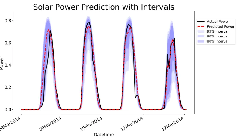
Figure 2.3 Solar Power Prediction with Intervals . . . 47

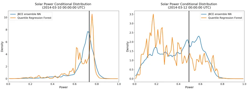
Figure 2.4 Solar Power Conditional Density . . . 48

Figure 3.1 Structures of Monotonic Guaranteed Neural Network . . . 58

Figure 3.2 Prediction Performance Comparison . . . 65

Figure 3.3 CRPS score change with fixed and adaptive sampling ofν . . . 66

Figure 3.4 Exploration of the electricity load dataset . . . 68

Figure 3.5 Prediction intervals for three different methods . . . 70

Figure B.1 Prediction Performance Comparison in AQTL (compared with QRF) 85 Figure B.2 Prediction Performance Comparison in CRPS (compared with DDR) 86 Figure B.3 Prediction Performance Comparison in AQTL (compared with DDR) 87 Figure B.4 AQTL score change with fixed and adaptive sampling ofν . . . 88

(13)

CHAPTER

1 NONPARAMETRIC VARIABLE SELECTION

FOR OPTIMAL TREATMENT DECISIONS

1.1 Introduction

Clinical trials are typically performed on a heterogeneous group of patients. Although the

goal of the trial is generally to assess the treatment effect over the entire population of

interest, sub-populations that respond differently to the treatment can exist. For many

treatments, often only a small proportion of the population will obtain the desired benefits,

(14)

heterogeneity can come from many sources, including patients’ diverse pharmacogenetic

backgrounds, medical histories, disease states and basic demographic information. Some

sources with known impact on the outcome can be taken into account in the design of

the trial, such as stratifying patients based on their gender and age[Kernan et al. (1999)].

However, the impact of many other characteristics are often unknown, or some

charac-teristics have not been measured, which results in diverse responses across the patients

within treatment groups. Understanding the sources of heterogeneity and being able to

characterize subgroups with different responses to the treatment is crucial in clinical

prac-tice, especially when alternative treatments are available. The advancement in genome

sequencing and the increased adoption of electronic health record system facilitate the

collection and maintenance of individual patient’s information, and provide an

opportu-nity for subgroup identification and characterization through statistical methods[Jensen

et al. (2012)]. This will allow for better prescription schemes and ultimately leads to the

maximization of treatment benefit at the individual level.

There are two related areas in the research of subgroup identification and

characteriza-tion in clinical trials. One of the areas is on the identificacharacteriza-tion of subgroups and proposing

treatment regimes that maximize the benefit for each subgroup[Song and Pepe (2004),

Bonetti and Gelber (2004), Kuk et al. (2010), Foster et al. (2011), Cai et al. (2011), Zhao et al.

(2013), Shen and He (2015) and Fan et al. (2017)]. Another area is on the identification

and selection of patients’ characteristics that are useful in subgroup identification. The

desired characteristics are those that not only interact with the treatment, but also have an

impact on the ordering of treatments. This type of interaction is often referred asqualitative

interaction, as opposed toquantitative interactionwhere patients’ characteristics interact

(15)

the identification and selection of qualitative interactions become crucial. Finding a subset

of baseline covariates that qualitatively interact with treatments can simplify the process of

subgroup identification. It can also reduce the cost of collecting and storing all the baseline

covariates from patients.

Our study is motivated by the AIDS Clinical Trials Group Study 175 (ACTG175)[Hammer

et al. (1996)]. The ACTG175 study was a randomized, double-blind, placebo-controlled trial

designed to compare the efficacy between monotherapies with zidovudine or didanosine

with combination therapies with zidovudine and didanosine or zidovudine and zalcitabine

in HIV-infected subjects. The main original finding is that the combination therapies are

su-perior to the monotherapy with zidovudine alone. It also appears that the two combination

therapies have very similar overall treatment responses at 96 weeks, measured by percent

change in CD4 cell count. It is not clear whether there exist subgroups in the population

that will benefit differently from the two combination therapies, and if such subgroups

exist, what are the covariates required to identify them. We aim to address these questions

and design a treatment policy to maximize the benefit to the patients.

Few methods have been proposed specifically to address variable selection problems in

treatment assignment decision making. Gunter et al. (2011) suggested a measure for

quali-tative interaction ranking, the S-score, and used it to rank and select subsets of covariates.

They then used forward selection and Average Gain Value (AGV) to select the final model.

Fan et al. (2016) pointed out that since this S-score measures the qualitative interaction for

each covariate marginally, it does not take into account the correlation among covariates.

Thus they proposed the Sequential Advantage Selection method (SAS), and used a BIC-type

criterion to select the best subset. Both methods assume that the relationship between the

covariates that have qualitative interaction and the treatment responses are linear.

In this article, we propose a general procedure for selecting subsets of covariates that

(16)

qualita-tive interactions of individual variables with the treatment, we adopt the regret function

introduced by Murphy (2003) to evaluate the optimal treatment policies from different

models with different subsets of covariates. Additionally, we develop a hypothesis test

based approach as our selection criterion, by approximating the distribution of the regret

function given the model. The advantage of our procedure is its compatibility with a variety

of models that can be used to model the treatment responses. In this research, we use

the Gaussian process as an example to model the response surface and demonstrate the

usefulness of our procedure. The choice of flexible models like Gaussian process can also

alleviate the limitations from linear model based approaches proposed by Gunter et al.

(2011) and Fan et al. (2016).

The remainder of this article is organized as follows: Section 1.2 introduces the optimal

treatment decision framework and the regret function. Section 1.3 details the selection

procedure and the criterion to choose the model. Section 1.4 describes the Gaussian process

model and estimation of the optimal treatment policy. Section 1.5 shows the comparison

between the SAS approach proposed by Fan et al. (2016) and our method in a simulation

study. Section 1.6 conducts the analysis on the ACTG175 dataset using our approach. Finally,

a discussion is given in Section 1.7.

1.2 Treatment Decision and Variable Value

1.2.1 Optimal Treatment Decision

In this article, we focus our attention on the scenario where every clinical trial patient

is subjected to one of the two treatments denotedA = 0 and A =1. Let Y ∈ Rdenote

(17)

health records, etc. The optimal treatment decision for the patient is a function of their

covariates:

a?(X) =arg max a

E[Y|X,A=a]. (1.1)

We also denote the value of the optimal policy asV?, which is the population average

response if the treatments are assigned based on the optimal treatment policy,

V?=

Z

E[Y|X,A=a?(X)]g(X)dX, (1.2)

whereg(X)denotes the covariates’ density function.

1.2.2 Value and Regret

Obtaining the optimal treatment decision specified in (1.1) requires allp covariates being

collected and the high-dimensional response functionE(Y|X,A)being estimated. Our goal is to remove covariates that play a negligible role in treatment decision assignment, and

keep the variables that have an impact on the optimal treatment decisions. For a subset of

variablesX_M ={Xj :j ∈ M }, whereM ⊆ {1, 2, . . . ,p}, leta_M∗ (X) =arg max a

E[Y|X_M,A= a]be the optimal policy among the class of policies that use only the information from

covariatesX_M. We denoteV_M as its value,

VM =

Z

E[Y|X,A=a_M∗ (X)]g(X)dX. (1.3)

V_M is the population average (over allp covariates) of expected response assuming

treat-ments are assigned following the treatment policya∗

M(X). Note that the expectation is still

(18)

for the decision rule. To determine the consequences of using the policya∗

M(X), rather

thana?(X), we denote the regretR_M as the regret function[Murphy (2003)]taking value at

a∗ M(X):

RM =V?−VM. (1.4)

Instead of measuring how mucha∗

M(X)differs froma?(X), the regretRM measures the

magnitude of change in the expected outcome due to those treatment decision mistakes.

LargeR_M values would indicate thatX_M is missing some important covariates that may

affect the optimal treatment decision and the treatment mistakes caused by the absence of

those covariates’ information may have significant impact on overall treatment outcome.

In a broad sense, the regret can be used to evaluate any pair of nested models, if we

defineR12=VM1−VM2, givenM2⊆ M1. By formulating a hypothesis test ofR12=0, we can determine whether the covariate subset_M₂contains sufficient information for decision making with respect to _M₁. In our specific application, we are always comparing the selected subset_M with the complete set of covariates, and determining whetherR_M =0. In order to examine through the various subsets of covariates, we can utilize forward, backward

or any other step-wise selection procedures, and any procedure would include five general

steps:

1. Model the response surfaceE(Y|X,A)for each treatment as a function of allp base-line covariatesX(full model). Modeling the treatment effects separately allows for a

hypothesis testing procedure we developed in Section 1.3.3.

(19)

(a∗ M(X)).

4. EvaluateV_M,V?andR_M through numerical integration.

5. Determine whetherR_M =0.

In Section 1.3 we will describe our variable selection procedure and a hypothesis test based

stopping criterion in detail, given we can model the response surface. In Section 1.4, We

demonstrate the use of Gaussian processes to model the response function and obtaining

a?(X)anda∗ M(X).

1.3 Backward Selection for Sufficient Covariates Subset

1.3.1 Desirable Properties for Response Surface Modeling

As mentioned in Section 1.2.2, the first step in the selection for the sufficient covariates

subset is to model the response surface under each treatment condition. Various regression

models can be used for this purpose, while the following properties are often desirable:

1. Models with intrinsic variable selection ability. Some collected covariates in clinical

trials may not contribute to treatment response in any treatment condition. It is

beneficial to perform a global screening to exclude non-relevant covariates.

2. Models that allow statistical inference for the estimated response surface. This will

allow us to estimate the sampling distribution of the difference surface between

treatment responses, or contrast function (Zhang et al. (2012)), and thus conduct

hypothesis test, forR_M =0.

3. Models that are flexible enough for non-linear contrast functions. This will alleviate

(20)

In Section 1.4, we will discuss the use of Gaussian processes for modeling the response

surface.

1.3.2 Backward Selection Procedure

As discussed in Section 1.2.2, the regret is defined by the value difference between the

optimal treatment decision and the treatment decision based on the reduced set of

covari-ates. Thus backward selection will be directly evaluating the regret of removing a subset of

covariates. Following is the backward selection procedure:

1. For each treatment condition, we fit a regression model with all covariates. This is

denoted as "complete" model_M_{c o m p l e t e}=_{1, 2, . . . ,p}.

2. For models that have intrinsic variable selection ability, we perform a screening step

to remove the variables that are irrelevant for the response in all treatment conditions.

3. Re-fitting the model for each treatment with the remaining variables. We denote this

as the "full" model_Mf u l l ⊆ Mc o m p l e t e.

4. We evaluate the treatment response surface at locations drawn from the joint

distri-bution of X. The joint distridistri-bution of X can be estimated separately or we can simply

use the observed data points. We then determine the difference in treatment effect

(contrast function values) at those locations and corresponding optimal treatment

assignment.

5. Repeat step 3 and 4 with "reduced" models which we constructed based on a backward

(21)

(b) At stepm≥1, the models to be considered are denoted asMj(m)=M(

m−1)_{\ {}_j_}_,

for everyj ∈ M(m−1)_. (c) Estimate the regret ˆR_M(m)

j as an estimate ofRM (m)

j by plugging into (1.4). Remove

the variable j with the minimum estimated regret at this step. The minimum

estimated regret at stepm is denoted as ˆR_M(m).

(d) Derive or simulate the sampling distribution of ˆRM(m)at stepm≥1, and test for

the null hypothesisRM(m)=0.

(e) Repeat (b) to (d), untilRM(m)=0 is rejected.

1.3.3 Hypothesis Testing for the Regret

As mentioned in Section 1.3.2, we propose a stopping criterion based on a test for the null

hypothesisH0:RM(m)=0 versus the alternative hypothesisHa:RM(m)>0 at each stepm≥1. We first describe the derivation of the approximated sampling distribution forR_M under

H0for any subsetM and then the p-value for hypothesis test.

Let f(X) be the response function that we are trying to estimate. ˆf (X, ˆθ) denotes

an estimate for the response function, whereθcan be estimable parameters associated

with a non-parametric model, such as coefficients in regression splines or the

length-scale parameters in Gaussian process. If we assume ˆθhas asymptotic Gaussian sampling

distribution, and there exists someµ_θ andΩ_θ such thatpn(θˆ−µ_θ) N(0,Ωθ), whereµθ is the asymptotic mean andΩ_θ is the asymptotic covariance, then the asymptotic conditional

distribution of ˆf (X, ˆθ)_|X =x would be Gaussian based on delta method, and can be denoted as ˆf(X, ˆθ)_|X=x_∼N[µf(x),σ2f(x)].

To determine the optimal treatment assignment, we need to obtain ˆf0(X, ˆθ0) and

ˆ

f1(X, ˆθ1)which are the estimates of the response functions for treatmentA=0 andA=1

(22)

our estimated optimal treatment assignment will be determined by the estimated contrast

function. For instance, if ˆC(X, ˆθ₀, ˆθ₁)<0, it means that patients with covariatesXare esti-mated to have larger response value (better response) in treatment 0 than treatment 1 and

we will assign the patient to treatment 0; otherwise, we will assign the patient to the

alter-native treatment 1. More formally, we have the policy as: ˆa?(X, ˆθ₀, ˆθ₁) =I[Cˆ(X, ˆθ₀, ˆθ₁)_≥0]. We could similarly obtain ˆa∗

M(X, ˆθM0, ˆθM1)for the reduced modelM, where ˆθM0and ˆθM1 are the estimated parameters of the reduced models for each treatment response surface

respectively.

Because we modeled the response surface for each treatment separately, we assume that

ˆ

f0(X, ˆθ0)|X=x

⊥⊥

fˆ1(X, ˆθ1)|X=x. We then derive the asymptotic conditional distribution

of ˆC(X, ˆθ₀, ˆθ₁)_|X=xas: ˆ

C(X, ˆθ0, ˆθ1)|X=x∼N[µf1(x)−µf0(x),σ

2

f1(x) +σ

2

f0(x)], (1.5)

whereµ_f₀(x)andµ_f₁(x)are the asymptotic means of ˆf0(X, ˆθ0)|X=xand ˆf1(X, ˆθ1)|X=x,

whileσ2

f0(x)andσ

2

f1(x)are the corresponding asymptotic variances. Similarly, we can obtain the conditional distribution for the contrast function denoted ˆCM(X, ˆθM0, ˆθM1)as in the

reduced model_M.

The sampling distribution of regretRM in (1.4) is induced by the sampling distributions

of the optimal treatment decisions ˆa?(X, ˆθ0, ˆθ1)and ˆa_M∗ (X, ˆθM0, ˆθM1)and their

correspond-ing contrast functions ˆC(X, ˆθ₀, ˆθ₁)and ˆC_M(X, ˆθ_M₀, ˆθ_M₁). Under the null hypothesisR_M=

0, it means that_∀X_n in the covariate space_X,R_M(X_n) =I[a?(X_n)₆=a∗

M(Xn)]· |C(Xn)|=0. In another word, it means that whenever there is a difference in the outcome for

(23)

sub-alent toC(Xn)·CM(Xn)≥0, ifCM(Xn)6=0. For the boundary case, whereCM(Xn) =0, under the null hypothesis, we assume the assignment based on the reduced model is

same as the assignment based on the full model. In practice, the conditional distribution

ˆ

C_M(X, ˆθ₀, ˆθ₁)_|X is a continuous distribution, where the event ˆC_M(X_n, ˆθ₀, ˆθ₁) = 0 has 0 probability. To satisfy the condition under the null hypothesis based on our model

specifi-cation, and assume the models of choice for the contrast functions are consistent, we will

need to have:

E[Cˆ(X, ˆθ₀, ˆθ₁)_|X]_·E[Cˆ_M(X, ˆθ_M₀, ˆθ_M₁)_|X]_≥0. (1.6) For computational convenience, we assume ˆC(X, ˆθ0, ˆθ1)and ˆa?(X, ˆθ0, ˆθ1)are fixed

quan-tity estimated from the full model, and ˆCM(X, ˆθM0, ˆθM1) is random. In order to

gener-ate empirical samples of ˆC_M(X, ˆθ_M0, ˆθM1)from its sampling distribution under the null

which meets the criterion in (1.6), for every instanceX_n in the covariate space_X such

thatE[Cˆ_M(X, ˆθ_M₀, ˆθ_M₁)_|X=X_n]_·E[Cˆ(X, ˆθ₀, ˆθ₁)_|X=X_n]<0, we adjustE[Cˆ_M(X, ˆθ_M₀, ˆ

θ_M₁)_|X=X_n] =0, while keeping the variance of ˆC_M(X, ˆθ_M₀, ˆθ_M₁)_|Xunchanged.

Thus under the null hypothesisH0, for every instanceXn, we takeS=10, 000 samples from the adjusted distribution of ˆCMH0(X, ˆθM0, ˆθM1)|X=Xn, and subsequently obtain the samples of ˆa∗

MH₀(X, ˆθM0, ˆθM1)|X=Xn. Withst h sample from the distribution of ˆa

∗ MH₀(X,

ˆ

θ_M0, ˆθM1)|X=Xn, we can calculate the corresponding sample of regret atXn, ˆR( s) MH0(Xn) as:

ˆ

R_M(s)_H

0(Xn) = ˆ

EY[Y|Xn,A=aˆ?(s)(Xn, ˆθ0, ˆθ1)]− (1.7)

ˆ

EY[Y|Xn,A=aˆ∗( s)

(24)

space as:

ˆ

R_M(s)_H

0 = 1

N

X

n=1

ˆ

R_M(s)_H

0(Xn), (1.9)

whereN is the number ofXnevaluated in the covariate space. The samples of ˆRMH₀

repre-sent its empirical distribution underH0. The proportion of samples that are larger than the

estimated ˆR_Mfor model_Mis taken as our estimated p-value. More formally, it is calculated as:

ˆ

pM = 1

S

X

s=1

I[Rˆ_M(s)_H

0 > ˆ

RM]. (1.10)

The proportion ˆp_M is the estimated p-value for testing the null hypothesisH0:RM =0 versus the alternative hypothesisHa:RM >0 for modelM.

To adjust for multiple comparisons in each step of selection, we apply Bonferroni

correction. If total oft models are considered at stepm≥1, then the Bonferroni corrected p-value is:tpˆM(m).

1.4 Gaussian Process Model for Treatment Response

1.4.1 Gaussian Process Model

The optimal treatment policy will depend on the difference between the two treatment

response functions. We model the response for each treatment separately, and then combine

the results to obtain the policy. Unlike Gunter et al. (2011) and Fan et al. (2016), we use

(25)

(2006)]to model each treatment response. As described in Section 1.3.1 and 1.3.3, statistical

inferences on the parameters and estimated response surface are crucial. To achieve such

purpose, we take the Bayesian approach for the parameter estimation, as the uncertainty

quantifications on the parameters are easier to obtain from posterior distributions than

from maximum likelihood based approaches. The Gaussian process model is specified as:

Y =f(X) +ε, (1.11)

wheref(X)is the response surface, andεis the white noise error with distributionN(0,τ2₎_.

The response surface has a GP prior with mean parameterµand covariance function:

Cov[f(Xi),f(Xm)] =δ2K(Xi,Xm) =δ2 p

Y

j=1

exp

−(xi j−xm j)

2

2`2

j

. (1.12)

The function K(Xi,Xm) gives the prior correlation between f(Xi) and f (Xm), while δ2 _{is the signal variance and}_`

j is the length-scale parameter for dimension j. A repa-rameterization fromδ2 _and_τ2 _{to the overall variance}_σ2 ₌_δ2₊_τ2_{and the signal-ratio}

γ=δ2_/₍_δ2₊_τ2₎_{allows for a conjugate prior on}_σ2_{. Priors for}_µ_,_σ2_and_γ_{are then specified}

asµ_∼N(0,σ2

µ), σ2∼inverse-gamma(a,b)andγ∼U(0, 1). For simulation studies and real data application in Section 1.5 and Section 1.6, the priors are specified withσµ=100,a =0.1 andb =0.1.

We also add an initial variable screening step to remove the variables that are not

important for the response in either treatment conditions. To do so, we adopt the approach

presented by Linkletter et al. (2006), which is inspired by the Stochastic Search Variable

Selection (SSVS) method of George and McCulloch (1993) to enable the variable selection

for the GP. Linkletter et al. (2006) suggested a reparameterization from `_j > 0 to ρ_j = exp(₋1/2`2

(26)

Therefore to perform variable screening we use the SSVS prior:

ρj =1−UjPj, Uj ∼U(0, 1), Pj ∼B e r n(p0). (1.13)

This prior specification meansρj has probability 1−p0to be exactly 1, which is equivalent

toXj being removed from the model.p0=0.5 was used in simulation studies and the real

data analysis. We use the posterior probability thatXj is included in the model,P(ρj <1|Y), to screen for globally irrelevant covariates.

1.4.2 Computational Details

We apply MCMC separately for each treatment group, and thus omit the treatment indicator

A from this section. We perform MCMC marginally over the treatment response surface

f(X), so thatY = (Y1,Y2, . . . ,Yn)T has likelihoodY ∼N(µ1,σ2Σ), whereΣ=γK(X,X) + (1−γ)I. The mean and variance parametersµandσ2have closed form full conditional posteriors and thus we use Gibbs sampling and update them as following:

µ|X,Y,σ2,ρ1, . . . ,ρp,γ ∼ N(µˆ, ˆσ2) (1.14) σ2

(27)

The corresponding parameters of the conditional posteriors are:

ˆ

µ= 1

T_Σ−1_Y

1TΣ−1₁+σ2 σ2 µ

ˆ σ2=1

T_Σ−1₁

σ2 +

1 σ2

µ

ˆ

a =a+n

2

ˆ

b =b +(µ1−Y)

T_Σ−1₍_µ₁

−Y)

2

Forγ andρ_j,_∀j ∈ {1, 2, . . . ,p}, there are no closed form conditional posteriors and we update them using the Metropolis–Hastings algorithm proposed by Savitsky et al. (2011).

For the initial covariates screening step, we run MCMC for 2500 iteration with 500 burn-in

samples. We fit the Gaussian process again for each treatment with the remaining variables

with 6000 MCMC iterations and 1000 burn-in samples.

1.4.3 Response Surface Estimation

For a new patient with covariatesX∗_{, the new expected response} _f₍_X∗₎_{and the}

observa-tions have joint distribution:

 

f(X∗)

Y

 ∼N



µ1, σ2  

γK(X∗,X∗) γK(X∗,X)

γK(X,X∗₎ _γ_K₍_X_,_X_{) + (}₁₋_γ₎_I

  

 (1.16)

We denoteΩ₁₁=σ2_γ_K₍_X∗_,_X∗₎_,_Ω

12=ΩT21=σ

2_γ_K₍_X∗_,_X₎_and_Ω

22=σ2[γK(X,X)+(1−γ)I].

Thus the expected response atX∗_{is estimated by:}

ˆ

(28)

As a function of X∗, ˆf(X∗) is the treatment response surface for determining the

opti-mal treatment policy. The predicted value ˆf(X∗₎ _{depends on hyperparameters} _µ_, _σ2_,

ρ= (ρ₁,ρ₂, . . . ,ρ_p)T_{, and}_γ_{. To account for parameter uncertainty, we can compute the} average prediction over the hyperparameters’ posterior distribution. However, to simplify

computation, we instead plug in their posterior means, since at this stage, we are only

interested in the point prediction.

1.4.4 Approximated Distribution of the Response Surface

As mentioned in Section 1.3.2 and 1.3.3, our stopping criterion in the backward selection is

based on the hypothesis test ofR_M =0, where the sampling distribution of ˆR_M will depend

on the sampling distribution of the response surface ˆf(X∗₎_.

We denote all the parameters in our Gaussian process model asθ= (µ,σ,ρ₁, . . . ,ρ_p,γ)T_, and assume they approximately follows multivariate Gaussian distribution:θ_∼N(µ_θ,Ω_θ), whereµ_θ is the posterior mean andΩ_θ is the posterior covariance. By delta method, the

asymptotic distribution of ˆf(X∗, ˆθ)would be Gaussian with following specifications:

ˆ

f(X∗, ˆθ)_∼N[µf(X∗),σ2f(X

∗_)] _(1.18)

whereµf(X∗) =Eθ[fˆ(X∗,θ)] = Eθ[µ1+Ω12Ω₂₂−1(Y −µ1)], as stated in (1.17) and can be

estimated by plugging in the posterior means ofθ.σ2

f(X

(29)

method:

ˆ σ2

f(X

∗_{) =[}∂fˆ(X∗, ˆθ)

∂θ ]

T

b

Ωθ[

∂_fˆ₍_X∗_{, ˆ}_θ₎

∂θ ] (1.19)

∂ _fˆ₍_X∗_{, ˆ}_θ₎

∂θ =

∂µˆ1

∂θ +

∂Ωb₁₂

∂θ Ωb

−1

22(Y −µˆ1)+

b

Ω12

∂Ωb

−1 22

∂θ (Y −µˆ1)−

∂µˆ1

∂θ Ωb

−1 22Ωb

T

12 (1.20)

∂Ωb

−1 22

∂θ =−Ωb

−1 22

∂Ωb22

∂θ Ωb

−1

22 (1.21)

With the approximated distribution of the response surface, we could follow the steps

in Section 1.3.3 to conduct the hypothesis test ofR_M =0.

1.4.5 Approximated Parameter Re-estimation for Backward Selection

The estimation of the regretR_M requires the estimation of the response surfaces of both

full and reduced models. We could refit the Gaussian process each time when a covariate is

removed during backward selection to obtain the reduced models, if computation capacity

allows. Note that each of these models is fitted separately, so it is fully parallelizable directly.

Alternatively, we also proposed an approximation method for parameter re-estimation.

Based on our model parameterization in Section 1.4.1,ρ_j =1 means covariatesXj is not included in the model. We setρ_j =1,_∀j ∈M¯={j ∈ {1, 2, . . . ,p}|j ∈ M }/ . We also fix the total varianceσ2_{at the posterior mean from full model ˆ}_σ2

f u l l, as we assume it does not change dramatically with different subsets of covariates included in the model. Denote

θ_M ={µ,γ}∪{ρk},∀k∈ M, andθ_M¯ ={σ}∪{ρj},∀j ∈M¯. We can re-estimate the posterior distribution ofθ_M using the conditional Gaussian distributionθ_M_|θ_M¯, and then compute

(30)

1.5 Simulation Study

We performed a simulation study to compare our method with the SAS approach[Fan et al.

(2016)]and study sensitivities to the tuning parameters in the backward selection

proce-dures. Additionally, we also included the non-linear random forest method to model the

responses for each treatment based on input covariates, and recommended the treatment

policy based on the predicted treatment response for each treatment. The random forest

approach does not involve the selection of sufficient subset of covariates. We consider

the following three models to generate both linear and non-linear contrast functions with

different number of observations (n) and variables (p). In all cases, treatmentA=1 orA=0

is randomly assigned to each observation with probability 0.5. The covariates are Gaussian

with mean 0 and covariancec o v(Xi,Xi+d) =0.7d. The white noise error for the response is ε∼N(0, 1). We consider these response surfaces:

Model 1:

f(X,A) =1+2X1−2X2+{0.1+2X1−1.8X9+1.6X10}A

Model 2:

f(X,A) =1+2X1−2X2+{2−0.5∗(1+|X1|)2+2 cos(2X9)+

3 sin(2X10)}A

Model 3:

(31)

All the treatment-covariates interaction terms are designed to be influential on the direction

of treatment effects, based on the different values the covariates will take. The underlying

interactions are linear in Model 1 and non-linear in model 2. Both models havep =10

covariates. Model 3 has both linear and non-linear interactions and also more covariates

(p=30).

The performance of each method is evaluated by following quantities:

1. Value Ratio (VR): VR is defined as following:

V R=

R

a?₍X)=aˆ_M∗ (X)|C(X)|g(X)dX

R

|C(X)_|g(X)dX . (1.22)

C(X)is the contrast function:C(X) = f(X,A =1)₋f(X,A =0). Larger VR indi-cates improved responses following the policy proposed by the selected model. VR is

estimated through numerical integration by evaluatinga?(X), ˆa_M∗ (X)andC(X)at

10, 000 points randomly drawn from joint distribution ofX, and calculated as:

V R=

P

|C(X)_|I(a?(X) =aˆ∗ M(X))

P

|C(X)_| . (1.23)

2. Error Rate (ER): Error rate is defined as the misassignment rate:

E R=

Z

a?₍_X_n₎₆₌aˆ∗ M(Xn)

g(X)dX. (1.24)

ER is also calculated from the 10, 000 points randomly drawn from the covariate space

X as:

E R= 1

10000

X

n=1

I(a?(Xn)6=aˆ_M∗ (Xn)). (1.25)

(32)

interac-tions have been included in the selected model.

4. Selected Variable Set Size (Size): the number of covariates selected in the model.

The performance of the random forest, SAS and our Gaussian process variable selection

procedure (GP) was evaluated against 100 different datasets. For the random forest, default

parameters inRpackage

randomForest

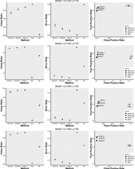
were used. Different p-value cutoffs for our

(33)

Figure 1.1: Simulation Results

(34)

selec-The simulation results showed that in the presence of non-linear qualitative interaction

(Models 2 and 3), policies derived from our GP backward selection procedure have better

treatment response and less assignment error compared to the SAS method. Also, our

method more often includes true qualitative interactions. The performance in the scenario

with only linear qualitative interaction (Model 1) also achieves good Value Ratio, Error Rate

and True Positive Rate, and only slightly inferior to the SAS method. In all the simulation

cases, our method has better Value Ratio and lower error rate than the random forest

method.

Our method with p-value cutoff atπ=0.1 generally gives an appropriate size close to the true size of important covariates, while forπ <0.1 seems to be conservative in selecting covariates into the model. The size of selected subsets in the SAS method is often greater

than the true size, indicating the inclusion of covariates with no qualitative interaction in

the model.

Increasing the ratiop/n also increases the treatment assignment error rate and de-creases the inclusion rate of true important qualitative interactions in our method. But the

Value Ratio, which reflect the overall quality of the policy, is not significantly affected.

1.6 Application to the ACTG175 Trial

We applied our proposed method to the dataset from AIDS Clinical Trials Group Study

175 (ACTG175). This study was conducted by Hammer et al. (1996) to compare the

treat-ment efficacy of monotherapy with zidovudine, and combination therapies in HIV-infected

adults with CD4 cell counts from 200 to 500 per cubic millimeter. The ACTG175 study was

(35)

zi-encing≥50% decline in CD4 cell counts at different time points. For modeling purposes, we used the ratio of the CD4 cell counts at 96 weeks to the CD4 cell counts at baseline as the

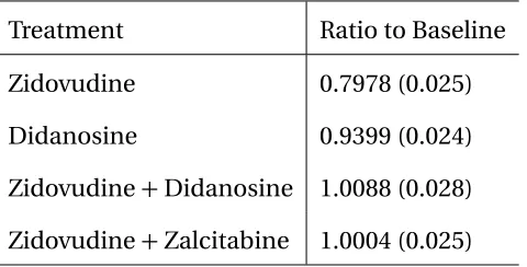
measure of treatment effect, and the result for each treatment is summarized in Table 1.1.

This rank of treatments is consistent with original conclusion from Hammer et al. (1996).

Table 1.1: Mean (standard error) of treatment effect at 96 weeks (ratio of 96-week and baseline CD4 cell count) for the ACTG175 study

Treatment Ratio to Baseline

Zidovudine 0.7978 (0.025)

Didanosine 0.9399 (0.024)

Zidovudine+Didanosine 1.0088 (0.028)

Zidovudine+Zalcitabine 1.0004 (0.025)

After the removal of missing observations, there are total 1104 patients who meet the criteria of baseline CD4 cell counts.

Though both combination therapies have superior treatment effects compared to single

treatments, their overall efficacies are very similar. Thus, the optimal treatment regime

may depend on baseline covariates of patients. In this dataset, there arep =16 baseline

covariates. We used Bayesian Gaussian process variable selection as described in Section

1.4 to model each treatment response and screen out variables that are not important for

(36)

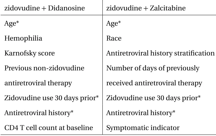
Table 1.2: Variables selected for each treatment by the Gaussian process regression model

zidovudine+Didanosine zidovudine+Zalcitabine

Age* Age*

Hemophilia Race

Karnofsky score Antiretroviral history stratification

Previous non-zidovudine

antiretroviral therapy

Number of days of previously

received antiretroviral therapy

Zidovudine use 30 days prior* Zidovudine use 30 days prior*

Antiretroviral history* Antiretroviral history*

CD4 T cell count at baseline Symptomatic indicator

Shared covariates in each treatment are labeled with *.

The data were then modeled with the covariates in Table 1.2 for each treatment using

GP regression again and we applied the backward selection procedure in Section 1.3 to

select the sufficient covariates subset. All the covariates that are considered in the backward

(37)

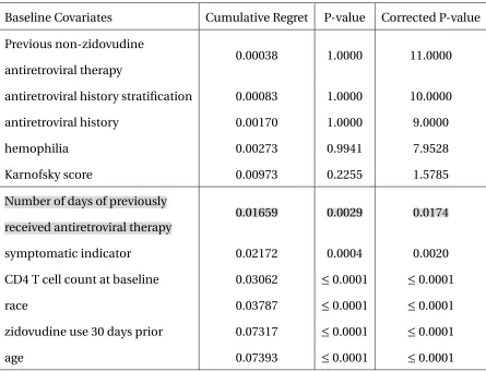
Table 1.3: Variables with qualitative interactions

Baseline Covariates Cumulative Regret P-value Corrected P-value

Previous non-zidovudine

antiretroviral therapy

0.00038 1.0000 11.0000

antiretroviral history stratification 0.00083 1.0000 10.0000

antiretroviral history 0.00170 1.0000 9.0000

hemophilia 0.00273 0.9941 7.9528

Karnofsky score 0.00973 0.2255 1.5785

Number of days of previously

received antiretroviral therapy

0.01659 0.0029 0.0174

symptomatic indicator 0.02172 0.0004 0.0020

CD4 T cell count at baseline 0.03062 _≤0.0001 _≤0.0001

race 0.03787 ≤0.0001 ≤0.0001

zidovudine use 30 days prior 0.07317 _≤0.0001 _≤0.0001

age 0.07393 _≤0.0001 _≤0.0001

Only ’number of days of previously received antiretroviral therapy’ (highlighted in gray) will be excluded from the selected covariates if we use p-value cutoff at 0.01. Since the performance of π=0.01 is less desirable from the simulation experiments, we usedπ=0.1 in this analysis.

The covariates in Table 1.3 are ranked in ascending order of the cumulative regret,

which is also the order of backward elimination, with top of the list being removed first. The

cumulative regret reflects the regret we will have by removing the corresponding covariate

together with all the covariates that have been removed in prior backward selection steps.

The p-value is calculated based on methods in Section 1.4.4 at each step and the Bonferroni

(38)

but any threshold greater than 0.0174 would give the same result. All the selected covariates

are listed below the line. In addition to age, which has previously been identified as an

important covariate for treatment assignment[Lu et al. (2013)], we also found several other

variables may be related to the treatment decision. Other than age and race, the selected

covariates are either about baseline health condition, such as CD4 cell count at baseline

and symptomatic indicator, or about previous usage of zidovudine. These information

could be valuable for further biological studies and the design of future clinical trials.

Qualitative interactions between selected covariates and treatment can be visualized in

the interaction plots in Figure 1.2 and Figure 1.3. We examined age and zidovudine usage 30

days prior to treatment in more detail in these interaction plots. Both covariates have effect

in individual treatment responses as indicated in Table 1.2, and have qualitative interactions

as shown in Table 1.3. Fitted response curves are plotted for each covariate in Figure 1.2.

Age and zidovudine usage 30 days prior marginally do not have qualitative interactions

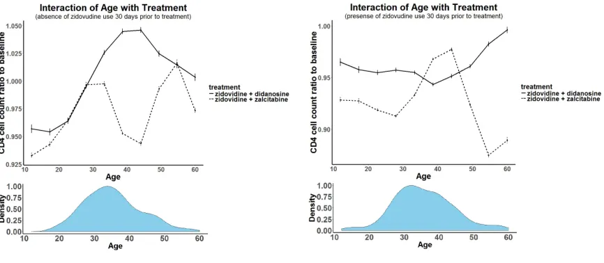
with treatment choices. However, as shown in Figure 1.3, conditional on the presense of

zidovudine usage 30 days prior, age has qualitative interaction with treatment choices.

In the group that is absent of previous zidovudine exposure, zidovudine+didanosine is

the superior treatment across all ages, while in the group that has previous zidovudine

exposure, zidovudine+zalcitabine will benefit patients between age 36 to 46. Just based on

the information from age and prior zidovudine usage, it affects optimal treatment policy

for 33.9% of patients in the group with prior zidovudine usage and 19.8% patients in total.

In high dimensions it is challenging to visualize the response surface. To illustrate the

estimated decision rule, we fit a decision tree with the selected covariates to approximate

our recommended treatment policy. More specifically, we fit a decision tree with the selected

(39)

Figure 1.2: Marginal Covariates-Treatment Interaction Plot

Treatment response surfaces are predicted based on GP regression for each treatment, and the marginal interaction plots are generated by integrating over other covariates through Monte Carlo integration. Standard error bars are also included.

Figure 1.3: Conditional Covariates-Treatment Interaction Plot

Interaction of age and treatment effects are plotted in subgroups stratified by zidovudine usage 30 days prior to treatment. The age distribution in each group is also provided.

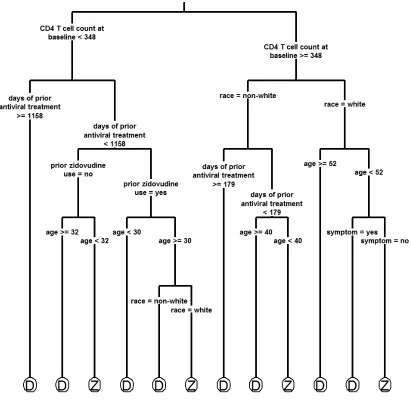
that while the zidovudine+didanosine combination is a slightly better treatment overall, if

a patient is young, has no symptom of disease or has relatively recent antiviral treatment,

then he/she may benefit from zidovudine+zalcitabine.

The biological relevance of selected variables are in general hard to be validated, unless

(40)

Figure 1.4: Decision tree approximation to the optimal treatment policy from Gaussian process (π=0.1)

Label D: the combination therapy of zidovudine+didanosine Label Z: the combination therapy of zidovudine+zalcitabine

the usefulness of the selected variables in subgroup identification and proposing optimal

treatment regimes. Thus, we compared the values of the treatment policy from our method

(41)

each method. We performed 5-fold cross validations for 10 rounds, and the results are shown

as the percentage of value increase comparing to the slightly inferior treatment: zidovudine

+zalcitabine. Results are summarized in Table 1.4. Following the policy suggested by our

method, we observe an improvement over the policy from SAS method.

Table 1.4: Percent value increase comparing to zidovudine+zalcitabine

Treatment Policy Percent Patients Treated with Z+D Value Increase

All treated with Z+D 100% 0.9

Policy from SAS 51.1% 0.9 (0.5)

Policy from GP* (π=0.1) 50.4% 1.9 (0.4)

Policy from GP* (π=0.05) 50.4% 1.6 (0.4)

SAS: sequential advantage selection. GP: Gaussian process variable selection procedure. Standard error is shown in the parenthesis. Z+Z: zidovudine+zalcitabine. Z+D: zidovudine+didanosine. Value Increase: 100×[(value of treatment policy)/(value of treating with zidovudine+ zalcitabine)-1]

* Selected covariates from Table 1.3 that have qualitative interactions with treatment assignments are used to model the difference of treatment response surfaces and decide the optimal treatment policy.

Although both methods will assign similar proportion of the patients to treatment

zidovudine+zalcitabine, their assignment policy only overlap by 63.7%, which indicates a

significant number of patients will be impacted with different assignment policies.

This case study showed that when two treatment options have very similar overall

bene-fit, it may differ in performance in subpopulations. Being able to construct an interpretable

treatment policy with a handful of selected patient covariates is crucial for clinical practices,

(42)

1.7 Discussion

In this paper, we propose a variable selection framework to select for subsets of covariates

that are sufficient for treatment decisions. This approach is based on the analysis of the

regret function of different reduced models. The proposed backward selection is used to

systematically identify the sufficient covariates subset and we design a hypothesis test for

the regret as the stopping criteria in the backward selection procedure. To demonstrate

the usefulness of our procedure, we use Bayesian Gaussian process model to estimate

the response surface for each treatment condition and make inference on the parameters

based on their posterior distributions. The proposed method is flexible to accommodate

non-linear relationship between covariates and treatment effects. The simulation study

shows that when there are non-linear components in the treatment contrast function,

our method outperforms linear model based approach in variable selection and provides

better treatment decision. Our method also selects key covariates that potentially impact

treatment decisions based on the AIDS Clinical Trials Group Study 175, and provides a

visual representation of the optimal treatment policy.

One drawback of our method is the computation time. Our method requires fitting

Gaussian process models for each treatment condition and can be time consuming when

there are multiple treatment groups or the number of patients(n)is large. Future work

could include the approximation techniques[Quinonero-Candela et al. (2007)]in Gaussian

process modeling and allow our method to be applied to larger problems. Alternatively,

other approaches that enjoy the properties in Section 1.3.1 can be used to replace Gaussian

(43)

CHAPTER

2 DEEP DISTRIBUTION REGRESSION

2.1 Introduction

In recent years, a variety of machine learning methods, such as random forest, gradient

boosting trees and neural networks have gained popularity and been widely adopted. These

methods are often flexible enough to uncover complex relationships in high-dimensional

data without strong assumptions on the underlying data structure. Off-the-shelf software is

available to put these algorithms into production[Pedregosa et al. (2011), Abadi et al. (2016)

and Paszke et al. (2017)]. However, in regression and forecasting tasks, many of the machine

(44)

regard-ing the uncertainty of the target quantity. Understandregard-ing uncertainties are often crucial

in fields such as financial markets and risk analysis[Diebold et al. (1997), Timmermann

(2000)], population and demographic studies[Wilson and Bell (2007)], transportation and

traffic analysis[Zhu and Laptev (2017), Rodrigues and Pereira (2018)]and energy

forecast-ing[Hong et al. (2016)]. In this article, we establish a framework that can directly extend

off-the-shelf machine learning algorithms to provide the full conditional distribution of

the response given the covariates. Instead of estimating specific quantiles[Koenker and

Hallock (2001), Taylor (2000) and Friedman (2001)], or prediction intervals[Khosravi et al.

(2011), Shrestha and Solomatine (2006)], we aim to directly estimate the full conditional

distribution, as other quantities can be directly extracted from it.

This research is motivated by the necessity of probabilistic prediction in energy

fore-casting. The Global Energy Forecasting Competition 2014[Hong et al. (2016)]focused on

probabilistic forecasting, due to the high demand of uncertainty estimation in energy

fore-casting, yet few existing methods are readily available. The solar energy forecasting track in

this competition aimed to estimate the full conditional distribution of solar energy

genera-tion based on covariates such as solar radiance, temperature, time of the day, etc. This is

a crucial task in actual day-to-day operation as solar energy generation is highly weather

dependent and thus volatile. To ensure stability in the electrical grid, grid operation not only

requires accurate point prediction of solar energy generation, but also its volatility based

on weather conditions. Driven by this practical problem, we establish a method to provide

comprehensive information regarding the energy generation uncertainties, by estimating

the full conditional distribution. Our method shows superior estimation accuracy in our

real data analysis compared to competing methods.

(45)

the conditional distribution estimate f(Y|X) =f(Y,X)/f(X). This approach is limited by the dimensionality of the input spaceX, due to having to estimate the full joint distribution

ofX. Several methods have then been proposed to address some of the limitations in both

locally parametric and non-parametric ways[Hyndman et al. (1996), Hyndman and Yao

(2002), Holmes et al. (2012), Fan et al. (2009), Izbicki and Lee (2016)]. Another popular

approach is to approximate the distribution of interest by a parametric distribution family

or mixture of such distributions, such as a mixture of Gaussians[Escobar and West (1995),

Song et al. (2004), Rojas et al. (2005), Fahey et al. (2007)]. This approach faces the challenge of

determining the number of mixtures, and the approximation performance will depend on

the complexity of the true underlying distribution. Bootstrap-based aggregation provides

an alternative method, and a good example is quantile regression forest[Meinshausen

(2006)], which obtains the full conditional distribution from the empirical distribution in

the aggregated tree leaves. A boosting approach to this problem was discussed in Schapire

et al. (2002).

Machine learning approaches have experienced major success in classification

prob-lems. We leverage this success to build conditional distribution estimates. In our paper,

we propose a two-stage method for conditional density estimation. In the first stage, we

partition the response space into bins; in the second stage, the probabilities that the target

variableY falls into each bin given the input covariatesX are estimated. In this way, we

transform a conditional density estimation problem into a multi-class classification task,

where we can take advantage of many off-the-shelf machine learning algorithms. This

framework enjoys the model-agnostic property in the second stage, allows for plugging

in any suitable multi-class classification method, such as deep learning for example. To

further accommodate the fact that the classes are ordered, we use a joint binary cross

entropy loss to couple with the neural network model. The design of our neural network

(46)

is not guaranteed by other ordinal classification methods as in Frank and Hall (2001) and

Cheng et al. (2008). In addition, we explore random partitioning in the first stage followed

by the ensemble approach to obtain a smoother and more stable density estimator.

The paper is organized as follows: In Section 2.2, we describe the model set up. In Section

2.2.1, we examine approaches and loss functions that can be used in the multi-class

classi-fication stage and in Section 2.2.2 we examine an alternative partition method and model

ensemble. In Section 2.3, we show that given the consistency of the classification model,

we can achieve consistency for the density estimator. We evaluate the model performance

with simulation studies in Section 2.4. In the simulation study, we thoroughly examine the

effect of number of bins, different binning strategies as well as different loss functions. In

Section 2.5, the method is illustrated using the aforementioned solar energy example where

we demonstrate superior performance to quantile random forests. We conclude with the

discussion in Section 2.6.

2.2 Distribution Estimation by Partitioning

Our approach is based on partitioning the range of the response variableY into bins and

approximating the conditional density functionf(y|X)by a piecewise constant function. We also propose ensemble random partitioning which allows for a smooth density. Formally,

assume we are interested in the density ofY in the range of[l,u]. This interval is partitioned

byK cut-pointsl <c1 <c2 <· · ·<cK <u into K +1 bins. Let c0 =l,cK+1=u andTk = [ck−1,ck)denotes thekth bin, fork ∈ {1,· · ·,K +1}.

(47)

form:

f(y|X)_≈

K+1

X

k=1

πk(X) |Tk|

I(y ∈Tk), (2.1)

where|Tk|=ck−ck−1is the size of the intervalTk.

We then estimateπ_k(X)with a classification model. Let ˆπ_k(X)be the estimator for πk(X)obtained from the classification model. Plugging ˆπk(X)into (2.1) gives the density estimator:

ˆ

f(y|X) =

K+1

X

k=1

ˆ πk(X)

|Tk|

I(y ∈Tk). (2.2)

A natural approach to estimateπ_k(X)is discussed in Section 2.2.1.

2.2.1 Probability Estimation for Each Partitioned Bin

Below we describe two different modeling strategies for the multi-class classification task

of estimatingπk(X).

Multinomial Log-likelihood

A natural approach to obtain the estimates for the conditional probability of a response

observation in each bin is to model the conditional distribution as a multinomial

distribu-tion. We note that this does not take into account the fact that the bins are ordered. We will

discuss how to deal with this fact in the next section. For a given observationX_n, where

(48)

whereπ(Xn;θ) = [π1(Xn;θ),π2(Xn;θ),· · ·,πK+1(Xn;θ)]is the probability vector describ-ing the conditional probability ofYn belonging to each bin givenXn, andθdenotes the

parameters in the classification model. The log-likelihood function is:

N

X

n=1

log_L(θ_|Yn,Xn) = N

X

n=1

K+1

X

k=1

I(Yn∈Tk)log[πk(Xn,θ)]. (2.3)

Given an appropriate classification modelπ(X;θ), our goal is to maximize the

log-likelihood function with respect toθ. In this work, we use deep neural networks as a flexible

and robust method. Under this model,θcorresponds to its biases and weights. The softmax

functionσ[z(Xn;θ)]i=ezi/

PK+1

j=1 e

zj_{was used as the activation function for the output layer}

of the neural network model, wherez(Xn;θ)is the output layer vector prior to the softmax

transformation. The softmax activation function ensures that the estimator ˆπ(Xn;θ)is a

valid probability vector, such that ˆπ_k(X_n;θ) =σ[z(X_n;θ)]_i>0 andPK+1

k=1πˆk(Xn;θ) =1.

Although we choose the neural network model, our framework is model-agnostic, and

any method that is appropriate for multi-class classification can be utilized. This approach

is very straight-forward in practice as many off-the-shelf machine learning tools have

multi-class multi-classification algorithms implemented. However, one potential caveat is that this

approach can be sensitive to the number of cut-pointsK. While largerK is required to

uncover the fine details of the target distribution and reduce bias, it results in increased

variance due to smaller number of observations per partitioned bin. Additionally, this

approach does not take the order of the bins into consideration. In order to address some

(49)

Joint Binary Cross Entropy Loss

Instead of utilizing multi-class classification to directly estimate the functionπ(X), we

reframe the problem asK binary classification tasks, and binary classifications are evaluated

at each of the K cut-points. In other words, we will obtain the conditional cumulative

distribution functionF(ck;Xn,θ) =P(Yn≤ck|Xn)by estimatingF(c1;Xn,θ),F(c2;Xn,θ), · · ·,F(cK;Xn,θ)jointly.

In this approach, we retain the model (i.e. neural networks) for the conditional

proba-bility thatYn belongs to each bin givenXn, but specify the loss function in terms of the

cumulative distribution functionF(ck;Xn,θ) =

Pk

m=1πm(Xn;θ). Because the estimates

ˆ

πk(Xn;θ)are positive, we are able to automatically obtain the monotonicity property of

F(ck;Xn,θ). For a given cut-pointck, the binary cross entropy (BCE) loss is:

B C E(ck) =− N

X

n=1

{I(Yn≤ck)log[F(ck;Xn,θ)]

+ [1₋I(Yn≤ck)]log[1−F(ck;Xn,θ)]}. (2.4)

Combining the BCEs across allK cut-points gives the joint binary cross entropy (JBCE)

loss:

J B C E =

K

X

k=1

B C E(ck). (2.5)

Our goal becomes minimizing the JBCE loss with respect toθ. This approach takes

the order of the bins into consideration in contrast to multi-class classification where the

Machine Learning Methods for Uncertainty Estimation and Decision-making.

ABSTRACT

DEDICATION

BIOGRAPHY

ACKNOWLEDGEMENTS

TABLE OF CONTENTS

LIST OF TABLES

LIST OF FIGURES

CHAPTER

1

NONPARAMETRIC VARIABLE SELECTION

FOR OPTIMAL TREATMENT DECISIONS

1.1

Introduction

1.2

Treatment Decision and Variable Value

1.2.1

Optimal Treatment Decision

1.2.2

Value and Regret

1.3

Backward Selection for Sufficient Covariates Subset

1.3.1

Desirable Properties for Response Surface Modeling

1.3.2

Backward Selection Procedure

1.3.3

Hypothesis Testing for the Regret

⊥⊥

1.4

Gaussian Process Model for Treatment Response

1.4.1

Gaussian Process Model

1.4.2

Computational Details

1.4.3

Response Surface Estimation

1.4.4

Approximated Distribution of the Response Surface

1.4.5

Approximated Parameter Re-estimation for Backward Selection

1.5

Simulation Study

randomForest

1.6

Application to the ACTG175 Trial

1.7

Discussion

CHAPTER

2

DEEP DISTRIBUTION REGRESSION

2.1

Introduction

2.2

Distribution Estimation by Partitioning

2.2.1

Probability Estimation for Each Partitioned Bin