Virtual Model Of A Vehicle Adaptive Damper System

(1)

University of Windsor University of Windsor

Scholarship at UWindsor

Electronic Theses and Dissertations Theses, Dissertations, and Major Papers

9-18-2019

Virtual Model Of A Vehicle Adaptive Damper System

Kyle Hugo

University of Windsor

Follow this and additional works at: https://scholar.uwindsor.ca/etd

Recommended Citation Recommended Citation

Hugo, Kyle, "Virtual Model Of A Vehicle Adaptive Damper System" (2019). Electronic Theses and Dissertations. 7810.

https://scholar.uwindsor.ca/etd/7810

This online database contains the full-text of PhD dissertations and Masters’ theses of University of Windsor students from 1954 forward. These documents are made available for personal study and research purposes only, in accordance with the Canadian Copyright Act and the Creative Commons license—CC BY-NC-ND (Attribution, Non-Commercial, No Derivative Works). Under this license, works must always be attributed to the copyright holder (original author), cannot be used for any commercial purposes, and may not be altered. Any other use would require the permission of the copyright holder. Students may inquire about withdrawing their dissertation and/or thesis from this database. For additional inquiries, please contact the repository administrator via email

(2)

VIRTUAL MODEL OF A VEHICLE ADAPTIVE DAMPER SYSTEM

By Kyle Hugo

A Thesis

Submitted to the Faculty of Graduate Studies

Through the Department of Manufacturing, Automotive, and Materials Engineering In Partial Fulfilment of the Requirements for

The Degree of Master of Applied Science at the University of Windsor

Windsor, Ontario, Canada

(3)

ii Virtual Model of a Vehicle Adaptive Damping System

By

Kyle Hugo

APPROVED BY:

______________________________________________ N. Kar

Department of Electrical and Computer Engineering

______________________________________________ B. Minaker

Department of Mechanical, Automotive, and Materials Engineering

______________________________________________ J. Johrendt, Advisor

Department of Mechanical, Automotive, and Materials Engineering

(4)

iii

Declaration of Originality

I hereby certify that I am the sole author of this thesis and that no part of this thesis has been

published or submitted for publication.

I certify that, to the best of my knowledge, my thesis does not infringe upon anyone’s copyright

nor violate any proprietary rights and that any ideas, techniques, quotations, or any other

material from the work of other people included in my thesis, published or otherwise, are fully

acknowledged in accordance with the standard referencing practices. Furthermore, to the

extent that I have included copyrighted material that surpasses the bounds of fair dealing

within the meaning of the Canada Copyright Act, I certify that I have obtained a written

permission from the copyright owner(s) to include such material(s) in my thesis and have

included copies of such copyright clearances to my appendix.

I declare that this is a true copy of my thesis, including any final revisions, as approved by my

thesis committee and the Graduate Studies office, and that this thesis has not been submitted

(5)

iv

Abstract

Several FCA vehicles are fitted with semi-active damper systems which modulate the level of damping

implemented in the vehicle suspension system to improve both the handling and ride quality felt by

vehicle’s occupants.

Durability simulations are necessary to analyze a vehicle’s or a component’s structural integrity over an

expected lifespan. Performing durability simulations in a virtual environment has streamlined the

traditional development cycle by reducing the need to construct physical prototypes and conduct

physical road or bench tests. It is essential that the vehicle is modeled as accurately as possible in the

virtual environment to ensure the results are representative of real-world performance.

Presently, the incorporation of a semi-active damper system in a virtual durability simulation involves

the expensive and resource intensive use of empirically obtained data. The goal of this project is to

improve the fidelity and efficiency of durability simulations by including the loading effects of a

semi-active suspension system. To accomplish this, several semi semi-active suspension control algorithms and

practical considerations are studied. Using a car model developed in Simulink©, a neural network,

clipped optimal control, and sliding mode control algorithms are developed to approximate operating

characteristics of the supplier controller. The development of each controller, along with appropriate

tuning and validation procedures in Simulink©, are presented.

A process known as co-simulation is then used to integrate each of the chosen semi-active damper

control systems into durability simulations used in vehicle development processes at FCA. Co-simulation

is a process wherein the controller is executed in parallel with MSC Adams© CAE durability simulation

software using Matlab©/Simulink©. The accuracy of the neural network, sliding mode controller, and

clipped optimal controller are validated by correlating results to a Co-simulation carried out with a

supplier controller.

It is found that the performance of the neural network controller resulted in output chattering

throughout the simulation. While performance is acceptable in ranges where the output data is

expected to be low frequency and low amplitude, instances where this was not the case induced

chattering events. These events are most likely due to the neural network receiving inputs outside of the

(6)

v

Dedication

I would like to take a hot minute to thank all the CAE simulation staff at FCA that put up with my

incessant questions and disasters, including; Chandra Tangella, Khanh Nguyen, Daniel Liang and Ali

Jahroumi. I would also like to thank Marie Mills of ARDC and Dr. Jennifer Johrendt of the University of

Windsor for always trying their hardest to keep this program running smoothly.

However, this thesis is dedicated to Reza Atashrazm, without whose help and unfailing patience, I would

still be trying to open a .adm file in Motionview.

(7)

vi

List of Figures

Figure 1: The damping stiffness of a vehicle is chosen based on its intended use... 1

Figure 2: Active suspension quarter car model with force actuator in parallel with spring and damper elements [1] ... 2

Figure 3: Semi-Active suspension quarter car model with adjustable damper [1] ... 2

Figure 4: Discrete semi-active damper curves (Jounce negative) ... 5

Figure 5: Damper curve selection algorithm for hybrid durability simulations ... 6

Figure 6: Comparison of durability simulation damper force methods: Direct (red), Using voltage output in conjunction with damper curves (blue) ... 7

Figure 7: Skyhook model ... 9

Figure 8: Quarter car model used for controller development in [8] and [9]. ... 11

Figure 9: 2-5-1 MLP Neural network [2] ... 16

Figure 10: schematic of ith_{perceptron and activation function [2] ... 16}

Figure 11: Sigmoid tangent activation function [10]. ... 17

Figure 12: General network schematic for gradient descent training method explanation [2] ... 18

Figure 13: Histogram of network weights used to evaluate network quality [2]. ... 19

Figure 14: Reference Skyhook damping model [12] ... 21

Figure 15: Simulink© Optimal controller and quarter car model diagram ... 25

Figure 16: Time domain plot of vertical sprung body acceleration of quarter car models with clipped optimal controlled and passive damping ... 26

Figure 17: Time domain plot of damper force of quarter car models with clipped optimal controlled and passive damping ... 27

Figure 18: Vertical sprung mass body acceleration estimated amplitude spectrum of Clipped optimal controlled damping and passive damping ... 28

Figure 19: Full car Simulink© model with clipped optimal controller ... 29

Figure 20: Clipped optimal control damper output curve selection Simulink© Model ... 30

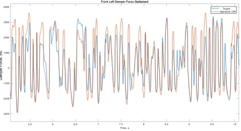
Figure 21: Front left damper force time history curve of Pattern Search optimized clipped optimal controller and supplier controller ... 31

(11)

x Figure 23: Rear left damper force time history curve of particle swarm optimized clipped optimal

controller and supplier controller ... 33

Figure 24: Training road input dataset ... 35

Figure 25: Matlab© GUI for creating neural networks ... 36

Figure 26: Baseline neural network architecture, a visual representation ... 36

Figure 27: 11-20-4 network test: ISO 2681 D-Class road profile ... 38

Figure 28: 11-20-4 network test: ISO 2681 B-Class road profile ... 38

Figure 29: 11-20-4 network test: Step Input ... 39

Figure 30: Road profile used to create more relevant training data ... 40

Figure 31: Best performing neural network for rough road - HPcSns1_ruf_FL ... 42

Figure 32: Durability road amplitude spectrum (OG) and replicating transfer function (TF) ... 43

Figure 33: Durability road PSD (OG) and replicating transfer function (TF) ... 44

Figure 34: Training, Validation, and Test Data similar to the durability road profile ... 45

Figure 35: Best performing neural network the durability road transfer function - PcSns3_RT_FL ... 47

Figure 36: Simulink© SMC model diagram ... 48

Figure 37: Time history of vertical body acceleration and damper force for SMC and passive systems ... 50

Figure 38: Sprung body mass vertical acceleration amplitude spectrum ... 51

Figure 39: Damper force amplitude spectrum... 51

Figure 40: Full car Simulink© model with individual corner SMC block ... 53

Figure 41: Half car SMC controller reference model ... 54

Figure 42: Full car Simulink© model controlled by two half car based sliding mode controllers ... 57

Figure 43: Time history results of individual wheel sliding mode control tuned with pattern search optimization ... 59

Figure 44: Time history results of half car model based Sliding Mode control tuned with Pattern Search Optimization ... 61

Figure 45: Adams© State Variable setup window for damper force plant input ... 64

Figure 46: Adams© State Variable setup window for plant outputs ... 64

Figure 47: Adams© direct single component force element specification window - Front ... 65

Figure 48: Adams© direct single component force element specification window - Rear ... 65

Figure 49: Original passive damper element ... 66

(12)

xi

Figure 51: Full vehicle analysis file driven event setup window ... 67

Figure 52: Adams©/Controls Plant Export window ... 68

Figure 53: Matlab© workspace generated by executing the .m file from the plant export utility ... 69

Figure 54: Matlab© command window Adams© plant actuators (inputs to Adams©) and sensors (outputs from Adams©) after running .m file from the plant export utility ... 69

Figure 55: .m file required modifications for Linux... 69

Figure 56: Generated Adams_sys.slx file containing Simulink© blocks linking to Adams© model ... 70

Figure 57: Passively damped Adams© Co-simulation Simulink© model ... 71

Figure 58: Co-simulation configuration parameters setup window ... 72

Figure 59: Block diagram within adams_sub block ... 73

Figure 60: adams_plant block parameters ... 73

Figure 61: Damper velocity plot of passive system executed purely in Adams© (red) and using Co-simulation, measured with built in damper output (blue) and measured with output state variable (pink) ... 74

Figure 62: Damper force plot of passive system executed purely in Adams© (red) and using Co-simulation (blue). The overlap of the two outputs indicates that the points in which velocity is measured from does not hinder damper force implementation ... 74

Figure 63: Supplier controller co-simulation acceleration output marker declaration ... 77

Figure 64: Supplier controller co-simulation body acceleration plant output state variable declaration . 77 Figure 65: Supplier controller co-simulation vertical body - wheel relative displacement plant output state variable declaration ... 77

Figure 66: Simulink© block diagram for Adams© co-simulation with supplier controller ... 78

Figure 67: Simulink© block diagram for Adams© co-simulation with neural network controllers ... 79

Figure 68: Linear regression plots between neural network controlled and supplier controlled dampers at each vehicle corner. ... 81

Figure 69: Front left damper force time history output - Neural network controller and supplier controller... 82

Figure 70: Front right damper force time history output - Neural network controller and supplier controller... 83

(13)

xii Figure 72: Rear Right damper force time history output - Neural network controller and supplier

controller... 85

Figure 73: Overall Max/Min loads output by dampers comparison ... 87

Figure 74: Damage ratio - Neural network controller versus Supplier controller ... 88

Figure 75: Simulink© full car ride model schematic ... 99

Figure 76: Wheel Equation of motion (46) Simulink© Model ... 102

Figure 77: Vehicle body Equations of motion (48), (49), & (50) Simulink© model ... 103

Figure 78: Centroid accelerations to corner displacement conversion Simulink© block ... 103

(14)

xiii

List of Tables

Table 1: SMC gain example values [12] ... 22

Table 2: Clipped optimal controller tuning weights ... 26

Table 3: Error results of clipped optimal controller with pattern search optimized weights ... 31

Table 4: Error results of clipped optimal controller with particle swarm optimized weights ... 33

Table 5: Neural Network input and output data channels ... 34

Table 6: Initial neural network training parameters ... 36

Table 7: Initial neural network perceptron sensitivity ... 37

Table 8: Initial neural network layer sensitivity ... 37

Table 9: FL Damper Neural network layer size sensitivity for rough road input ... 41

Table 10: FL Damper Neural network layer size sensitivity for rough road input with History ... 41

Table 11: FL Damper Neural network layer size sensitivity for the durability road transfer function input ... 46

Table 12: FL Damper Neural network layer size sensitivity for the durability road transfer function input with history inputs ... 46

Table 13: Quarter car simulation parameter values [12] ... 49

Table 14: Optimized quarter car model-based SMC tuning parameters ... 58

Table 15: Error results of quarter car model based Sliding Mode Control tuned with Pattern Search Optimization ... 59

Table 16: Half car model based sliding mode controller optimized controller tuning parameters ... 60

Table 17: Error results of half car model based Sliding Mode Control tuned with Pattern Search Optimization ... 61

Table 18: Semi-active damper force linear regression – Neural network controller ... 80

Table 19: Overall Max/Min loads output by dampers - Supplier controller ... 87

Table 20: Overall Max/Min loads output by dampers - Neural Network controller ... 87

Table 21: Calculated damage for 100 cycles - Neural network controller ... 88

(15)

xiv

List of Variables

𝐴 State space state matrix

𝐵 State space input to state matrix

𝑏_𝑖 Neural network bias for perceptron i

𝐶 State space to output matrix

𝐶𝑑𝑝 Passive damping

𝐶_𝑆𝑘𝑦 Skyhook damping coefficient

𝐶_𝑡 Tire damping

𝐷 State space feed through matrix

𝑒 Sliding mode control actual – ideal system error 𝑓𝑑0 Sliding mode control base desirable damping force

𝐹𝑠 Damper force state space input vector

𝐹𝑆𝐷 Corner spring + damper force

𝐹_𝑆𝑘𝑦 Skyhook damping force

𝐼_𝜙 Sprung body pitch inertia

𝐼_𝜃 Sprung body roll inertia

𝐽 Optimal control cost function

𝐾 Sliding mode control gain

𝑘𝑠 Spring stiffness

𝑘_𝑡 Tire stiffness

𝑀_𝑏 Sprung body mass

𝑀_𝑤 Unsprung wheel mass

𝑁 Complete state vector to damper velocity conversion

𝑄 Optimal control state weight matrix

𝑅 Optimal control input weight matrix

𝑆 Sliding mode control sliding surface

𝑢 Controlled corner damper force

𝑤𝑖,𝑗 Neural network weight for perceptron i and input j

𝑋 State space state vector

𝑥𝑖 Neural network input

𝑦_𝑖 Neural network output

𝑧_𝑏 Sprung body mass vertical displacement

𝑧_𝑟 Road input vertical displacement

𝑧_𝑤 Unsprung wheel mass vertical displacement

𝛼 Neural network momentum

𝜂 Neural network learning rate

𝜃_𝑏 Sprung body mass roll displacement

𝜙_𝑏 Sprung body mass pitch displacement

(16)

xv

List of Abbreviations

1. FCA – Fiat Chrysler Automobiles

2. LQR – Linear Quadratic Regulator

3. SMC – Sliding Mode Control

4. ADS – Adaptive Damper System

5. FLC – Fuzzy Logic Controller

6. PSV – Passive

7. PSD – Power Spectral Density

8. GUI – Graphic User Interface

9. NN – Neural Network

10. FL – Front Left

11. FR – Front Right

12. RL – Rear Left

13. RR – Rear Right

Note on Confidentiality

Due to confidentiality concerns concerning the contents of this work in regards to Fiat Chrysler

(17)

1. Introduction

To remain competitive in today’s global vehicle market, several FCA vehicle offerings are fitted with

advanced suspension systems. These systems have the capability of modifying suspension parameters to

improve comfort or handling based on a given road condition and driver preferences.

1.1. Background

1.1.1. Active and Semi-Active Suspension Systems

Comfort and handling are two conflicting performance objectives faced in the design of any vehicle’s

suspension system [1]. A damping setting with a higher damping coefficient can improve handling by

quickly dissipating oscillations. Conversely, a softer damping setting that dissipates less energy via a

lower damping coefficient reduces the magnitude of accelerations felt by the occupants in the sprung

vehicle body, thus improving perceived comfort. In a passive suspension system this introduces a

compromise that must be addressed based on the desired performance of the vehicle. Figure 1 shows a

Chrysler Pacifica, which focuses on providing a comfortable ride, which is partially accomplished with

soft dampers. Conversely, Figure 1 also shows a Formula Drift Spec Nissan S15 Silvia that must provide

precise handling to remain competitive, partially accomplished by a stiff suspension setup.

Figure 1: The damping stiffness of a vehicle is chosen based on its intended use.

Controllable suspension systems offer a solution to negate this compromise, by being able to adjust the

suspension’s characteristics depending on the driving situation. The field of controllable suspension

systems may be divided into two main categories: active suspension systems, and semi-active

suspension systems.

Active suspension systems feature a controllable force actuator which is placed between the sprung and

unsprung masses either in parallel with the spring and passive damper, as represented with a quarter

(18)

2

Figure 2: Active suspension quarter car model with force actuator in parallel with spring and damper elements [1]

In an active suspension system, energy is added to the system via the force actuator element. This is

advantageous as the desired control force output does not depend on the relative motion between the

sprung and unsprung masses. The downsides seen with implementing active suspension systems are the

system complexity with the addition of the actuation system along with the power requirements

required to realize it. These power requirements are typically in the range of 4-20 kW [1], which are

impractical due to the necessity to draw this power from the vehicle’s powertrain.

A less complex alternative to active suspension systems are semi-active suspension systems, also known

as adaptive damper systems (ADS). In this case, the damper has the ability to modulate the amount of

damping that is imposed on the system. Figure 3 denotes a quarter car model featuring a semi-active

suspension system.

(19)

3 Semi-active suspension systems may be further decomposed into two categories. The first category are

systems with continuously variable damping, where the damping coefficient can take any value between

an upper and lower limit. These systems are typically realized with magnetorheological dampers. The

second category consists of systems where the dampers are adjustable between two or more discreet

damping levels. These systems are typically realized with fluid dampers that have the ability to modulate

the valve orifice size. For the remainder of this work, dampers with the ability to modulate between

discreet damping levels will be considered, as commonly deployed on FCA products.

The largest advantage with adaptive damper systems is their relative simplicity to implement. The only

additional hardware required beyond the switching damper itself are additional sensors for body

accelerations along with the controller itself. Furthermore, the energy requirement for a semi-active

damper system is only in the range of 80 – 160W [1].

Regardless of the type of intelligent suspension system chosen, a control algorithm is always required in

order to modulate the system to extract the desired performance benefits from the vehicle. A main

focus of this work is devoted to evaluating two commonly employed control strategies, which are

further discussed in Chapter 2.

1.1.2. Vehicle Durability Testing

To streamline the vehicle development process, virtual durability simulations have become a staple in

the automotive industry. Vehicle durability testing is conducted to evaluate the magnitude and direction

of loads imposed on a vehicle during the early development stages. This practice is required to validate

existing designs, both in terms of overall structural integrity and the fatigue life of the component [2].

The overall goal is to ensure vehicle components meet quality and longevity requirements in a

cost-effective manner.

Durability simulations may be divided into three main categories, the first is real world full vehicle

testing. In this case, a vehicle outfitted with an array of sensors and instruments is driven on a proving

ground to obtain the desired data. While this gives a very accurate representation of real world

conditions, the disadvantage is the fact that an operational vehicle prototype is required. This is a large

time and monetary investment, and as such is reserved for the latter stages of product development,

close to a vehicle’s production launch.

The second main category of durability simulations consists of those conducted on specialized test rigs.

(20)

4 The key advantage to test rig simulations is the controlled environment in which they are performed,

aiding in improving the repeatability of results. However, much like full car simulations, a drawback is

that a physical vehicle or component is required to conduct the experiment.

The previous two methods of durability testing both have the drawback that a physical vehicle or

component is requirement before the simulation may be performed. Usually, these physical examples

are only available in the later stages of product development, where product changes are costly to

effect. The third category of durability simulations takes place in a virtual environment, eliminating the

requirement for a physical prototype. An additional advantage to virtual durability testing is the speed

at which cyclic process of testing, analysis, modification, and retesting may be executed. Moreover, the

fact that this process may be executed in the early phases of the design cycle results in expense

reductions. This is because changes can be made, and designs may be optimized before resources are

invested into the construction of physical prototypes.

A disadvantage of virtual durability simulations is the necessity that the virtual model must be

representative of the physical component or vehicle. Modelling complex machinery assemblies, like

automobiles, requires simplifications and assumptions. In the case of durability simulations, steps must

be taken to reduce these assumptions and increase the fidelity of the models used. Examples include

more accurate bushings models [2], including flexible bodies, and in the case of this work, integrating

the effects of semi-active suspension systems. Doing so helps to ensure that results from simulation will

accurately reflect what will be seen when physical prototypes are tested on finalized designs.

1.1.3. Current Simulation Strategy

Semi-active suspension systems currently installed on FCA products are of the discrete modulation type

described in Section 1.1.1. In this case, each damper has a hard and soft setting for both rebound and

jounce travel. This implies that the damper may be in one of four possible settings, and therefore be

(21)

5

Figure 4: Discrete semi-active damper curves (Jounce negative)

The current method of incorporating the effects of a semi-active damper system into a full vehicle

durability simulation requires using measured data from an instrumented vehicle prototype. The

concept of this hybrid method is that a few accurate measurements obtained from a physical vehicle

bench test are incorporated into a virtual environment to produce an extensive set of load data that

would be otherwise difficult to physically measure.

In this case, two possible methods of incorporating semi-active dampers in durability simulations are

possible. In the first method, the loads reacted by each semi-active damper are measured and directly

put into the virtual simulation as an external force channel. The second method involves measuring the

voltage signal outputs from the semi-active suspension controller for each damper. From that point, the

algorithm shown in Figure 5 is utilized to choose the damper setting based on each measured voltage

signal. Finally, the measured velocity from the virtual durability simulation may be used with the

(22)

6

Figure 5: Damper curve selection algorithm for hybrid durability simulations

Figure 6 depicts a plot of the output of the two current methods of inputting damper force to a

durability simulation. Clearly, the method of using the controller voltage signal in conjunction with the

algorithm shown in Figure 5 and damper curves shown in Figure 4 (blue) closely matches curves

(23)

7

Figure 6: Comparison of durability simulation damper force methods: Direct (red), Using voltage output in conjunction with damper curves (blue)

This result proves that it is feasible to use preset damper force - velocity lookup curves along with some

form of control algorithm to effectively replicate the output of the supplier’s unknown control structure

in durability simulations.

1.2. Project Motivation

Currently, accurate vehicle durability simulations involving semi-active damping systems require that in

initial full vehicle simulation be conducted to determine the characteristics of a semi-active damper

control system.

As stated in the background Section above, two possible solutions exist for implementing semi-active

damper systems within virtual durability simulations at FCA. The first solution requires data from road

test simulations, which is not feasible due to the need to implement virtual simulations before the

construction of prototypes. The second solution assigns a hard damper setting throughout the entire

simulation. This method is inaccurate as damper forces are then overestimated, which leads to the

overdesign of components. These two methods are not sufficient to meet today’s vehicle quality

standards, providing motivation for the current research project that will refine the results of vehicle

(24)

8 To date, there have been several logical reasons why the effects of a semi-active damper system have

not been incorporated into virtual durability simulations. The first, and most prevalent, is that the

controller structure is proprietary to the original supplier of the semi-active damper system. As such it is

not available in detail to be examined by FCA. As such, it is required that this work develop its own

control algorithm capable of replicating both this supplier’s controller as well as any implemented going

forward.

Another key reason as to why a respective controller algorithm has not been acquired by FCA, is that

instances where it has been critical to understand semi-active damper controller effects on vehicle

performance often only consider a singular event. Examples include hard acceleration, heavy braking, a

moose test, etc. In these events, it is far easier to track the state of the damper throughout due to the

short time duration. This situation differs from a full durability simulation which consists of a complete

road profile composed of many events over a long period of time.

1.3. Organization of the Thesis

Chapter 2 of this work contains a literature review containing the semi-active suspension control

techniques chosen in this work. These control techniques include clipped optimal control, neural

networks, and sliding mode control. The mathematical background of each of these control strategies is

explored, and performance results from literature sources are displayed.

Moving forward, Chapter 3 focuses on Simulink© controller modelling. The performance of clipped

optimal and sliding mode controllers are examined using a quarter car model. A Simulink© full car ride

model is developed and used to examine controller performance and to efficiently tune controller

parameters using optimization techniques. This same full car ride model is used to generate data in

order to create neural network controllers. Finally, final controller structures are chosen for

co-simulation.

Chapters 4 and 5 bring the union of the control structures developed in Simulink© to virtual durability

simulations in MSC Adams©. First, in Chapter 4, an Adams© model is modified to integrate semi-active

suspension with co-simulation. Methodology for how control structures chosen in Chapter 3 are

integrated into durability simulations using co-simulation is discussed in Chapter 5.

Chapter 6 presents the results for how well the selected control algorithms perform in conjunction with

the full car durability model when compared to a supplier controller. Chapter 7 goes on to include a

(25)

9

2. Literature Review

2.1. Skyhook Control

It is impossible to discuss semi active damping systems without mentioning the concept of Skyhook

damping. Skyhook control was one of the first control models developed for an adaptive damping

system in the 1970s by Karnopp et al. [3] and remains a commonly referenced model in the realm of

adaptive suspension design.

The conceptualization of the Skyhook model is the addition of a second damper to the quarter car

model that is attached to an imaginary fixed reference plane in the sky, as shown in Figure 7. The

addition of this secondary imaginary damper aims to improve the comfort of the vehicle occupants by

further reducing the transmissibility of road variation to the sprung mass.

Figure 7: Skyhook model

They hypothetical Skyhook control force acting on the sprung mass is realized according to the following

logic [4]:

𝐹_𝑆𝑘𝑦 = {𝐶𝑆𝑘𝑦𝑧̇𝑏 → 𝑧̇𝑏(𝑧̇𝑏− 𝑧̇𝑤) > 0

0 → 𝑧̇𝑏(𝑧̇𝑏− 𝑧̇𝑤) ≤ 0} (1)

𝑚

_𝑏

𝑚

_𝑤

𝑧

_𝑏

𝑧

_𝑤

(26)

10 It was determined via Simulink© simulation in [4] that the implementation of a simple Skyhook damper

controller dramatically reduced the transmissibility of a step road input to the vehicle unsprung mass,

and therefore the occupants.

Obviously, the idea of Skyhook control is impossible to implement on a real vehicle, but is considered as

a conceptual ideal system. Several methods have been deployed to practically implement this concept

however, using methods such as direct implementation [5], fuzzy logic [6] [7], and sliding mode control.

The latter is discussed in Section 2.5.

2.2. Clipped Optimal Control

[8] Focuses on the design and implementation of an optimal control scheme that goes beyond the

traditional input of only measured vehicle states. In this case, driver inputs such as braking, acceleration,

and cornering, in the form of inertial loads are considered mathematically as inertial forces acting on the

vehicle body. The purpose of this method is to create a more complete control structure, as the

controller can accommodate the additional large force variation on the suspension system implemented

by handling inputs.

2.2.1. Quarter Car

A modification is made to the quarter car model in [9] as can be seen in the Figure 8. The system

includes three inputs: damping coefficient, where: 𝑐𝑚𝑖𝑛∗ (𝑧̇𝑏− 𝑧̇𝑤) ≤ 𝑢 ≤ 𝑐𝑚𝑎𝑥∗ (𝑧̇𝑏− 𝑧̇𝑤), handling

inputs which are modeled as an external load 𝐹𝑠 applied to the body mass, and a road input that is taken

(27)

11

Figure 8: Quarter car model used for controller development in [8] and [9].

The quarter car model is described in state space using Equations (2) and (3) [9]. It is noted that body

and wheel displacements are taken relative to the road as opposed to absolute measurements. This is

done as it avoids estimation drift in further developments of a state estimator discussed in [9].

𝑥̇ = 𝐴𝑥 + 𝐵𝑁𝑇_{𝑥𝑢 + 𝐷𝐹}

𝑆+ 𝐺𝑧̇𝑟 (2)

[ 𝑧̇_𝑏− 𝑧̇_𝑟 𝑧̈_𝑏 𝑧̇_𝑤− 𝑧̇_𝑟 𝑧̈_𝑤 ] = [

0 1 0 0

− 𝑘𝑠 𝑚_𝑏 0

𝑘_𝑠

𝑚_𝑏 0

0 0 0 1

𝑘𝑠

𝑚𝑤 0 −

𝑘𝑠+ 𝑘𝑡

𝑚𝑤 0]

[ (𝑧_𝑏− 𝑧_𝑟) 𝑧̇_𝑏 (𝑧_𝑤− 𝑧_𝑟) 𝑧̇𝑤 ] + [ 0 − 1 𝑚_𝑏 0 1 𝑚_𝑤 ]

[0 1 0 −1] [

(28)

12 The performance index shown in Equation (4) is chosen in [8] as the basis for the optimal control

scheme is minimized over the control damper force input 𝑢. The first, second, and fourth terms are

related to comfort and performance objectives, whereas the third and fifth terms are included for

tuning flexibility.

𝐽 = 𝐸[1

2∫ (𝑞0𝑧̈𝑏2+ 𝑞1(𝑧𝑏− 𝑧𝑟)2

𝑇 0

+ 𝑞2𝑧̇𝑏2+ 𝑞3(𝑧𝑤− 𝑧𝑟)2+ 𝑞4𝑧̇𝑤2 + 𝑟𝑢2) ]

(4)

In state space form, the cost function in Equation (4) may be represented as shown in Equation (5).

𝐽 = 𝐸[1 2∫ [

𝑧 𝑢 𝐹𝑠 ] 𝑇 [

𝑄 𝑀₁ 𝑀₂ 𝑀₁𝑇 _𝑅

1 𝑀3

𝑀2𝑇 𝑀3𝑇 𝑅2

] [ 𝑧 𝑢 𝐹𝑠 ] 𝑇 0 ) ] (5)

The parameters 𝑞0, 𝑞1, 𝑞2, 𝑞3, 𝑞4 are tuned to adjust controller performance in terms of how the optimal

control law will target the states associated with each weight. The parameter 𝑟 is varied to adjust the

magnitude of the control output relative to the inputs. Both [8] and [9] show with extensive

computations that the cost function from Equation (4) is minimized by the expression shown in Equation

(6) for an infinite horizon.

𝑢∗_{= −𝑅}

1−1[(𝐵𝑇𝑃 + 𝑀1𝑇)𝑥 − 𝐵𝑇𝜎 + 𝑀3𝑑] (6)

As every damper is physically limited to a maximum and minimum damping coefficient, [8] clips the

output control force determined in Equation (6) to a damping coefficient within the bounds [𝐶𝑚𝑖𝑛, 𝐶𝑚𝑎𝑥] as shown in Equation (7).

𝐶_{𝑑𝑜𝑝𝑡}= 𝑠𝑎𝑡_[𝑐_𝑚𝑖𝑛_,𝑐_𝑚𝑎𝑥]{(𝑁𝑇𝑥)−1𝑢∗} (7)

The parameters 𝑄, 𝑅1, 𝑀1 𝑀2, & 𝑀3 from the cost function in Equation (5) and used in Equation (6) are

based on the vehicle’s parameters defined in both [8] and [9] as shown in Equations (8) to (1112).

𝑄 =

[

𝑞1+ 𝑞0

𝑘_𝑠2

𝑚_𝑏2 0 −𝑞0

𝑘_𝑠2

𝑚_𝑏2 0

0 𝑞₂ 0 0

−𝑞₀ 𝑘𝑠

2

𝑚_𝑏2 0 𝑞3+ 𝑞0

𝑘_𝑠2

𝑚_𝑏2 0

0 0 0 𝑞4]

(29)

13 𝑅₁ = [𝑟 + 𝑞0

𝑚_𝑏2] 𝑁𝑇𝑁

(9)

𝑀1= −𝑀2= [ 𝑞0(

𝑘_𝑠

𝑚_𝑏2) 0 −𝑞0(

𝑘_𝑠 𝑚_𝑏2) 0]

𝑇

(10)

𝑀3= −𝑞0

1

𝑚_𝑏2 (11)

Controller tuning in this case means choosing desired weighting factors and then determining the

matrices 𝑃 and 𝜎 so Equation (6) may be solved.

The set of terms in Equation (6) that is multiplied by state vector 𝑥 is a feedback term based on vehicle

states. The matrix 𝑃 is determined according to chosen weighting factors in the cost function in

Equation (4). This is done by numerically solving the algebraic Riccati Equation as follows in Equation

(12).

𝑃{𝐴 − 𝐵𝑅−1_𝑀

1𝑇} + {𝐴 − 𝐵𝑅−1𝑀1𝑇}𝑇𝑃 − 𝑃𝐵𝑅−1𝐵𝑇𝑃 + {𝑄 − 𝑀1𝑅−1𝑀1𝑇} = 0 (12)

The second term seen in Equation (6) including 𝜎 is a feedforward term based on the inertial forces

subjected to the sprung mass. For a quarter car model, 𝑑 = 𝐹𝑠as only vertical motion is considered. For

an infinite horizon, [8] determines the matrix 𝜎 from the algebraic Equation shown below in Equation

(13).

[𝐴𝑇_{− 𝑀}

1𝑅−1𝐵𝑇− 𝑃𝐵𝑅−1𝐵𝑇]𝜎 + [𝑀2− 𝑀1𝑅−1𝑀3+ 𝑃(𝐹 − 𝐵𝑅−1𝑀3)]𝑑 = 0 (13)

Once both the terms 𝑃 and 𝜎 are determined, controller tuning is complete. At this point, Equation (6)

can be solved in the controller at each time step or sampling increment. This produces an optimal

damper force given the input states and applied loads.

2.2.2. Full Car Ride Model

The above set of Equations are also valid for a full car ride model, which is developed in [9] for optimal

control and applied in [8] for clipped optimal control. As before, displacements are taken relative to the

(30)

14 quarter car model, acceleration and suspension displacement parameters are targeted states to control,

and both sprung and unsprung mass velocities are included for tuning flexibility [9] in the full car cost

function is shown in (14).

𝐽 = 𝐸[1

2∫ (𝑞0𝑧̈𝑏2+ 𝑞1𝜃̈𝑏2+ 𝑞2𝜙̈𝑏2+ 𝑞3𝑧̂𝑏2+

𝑇

0 𝑞4𝑧̇𝑏

2_{+ 𝑞}

5𝜃̂𝑏2+ 𝑞6𝜃̇𝑏2+ 𝑞7𝜙̂𝑏2+ 𝑞8𝜙̇𝑏2

+ 𝑞₉𝑧̂_𝑤2₁_{+ 𝑞} 10𝑧̇𝑤1

2 _{+ 𝑞} 11𝑧̂𝑤2

2 _{+ 𝑞} 12𝑧̇𝑤2

2 _{+ 𝑞} 13𝑧̂𝑤3

2 _{+ 𝑞} 14𝑧̇𝑤3

2 _{+ 𝑞} 15𝑧̂𝑤4

2

+ 𝑞₁₆𝑧̇_𝑤2₄_{+ 𝑞}

𝑢(𝑢12+ 𝑢22+ 𝑢32+ 𝑢42)𝑑𝑡) ]

(14)

Determining optimal controller outputs for damping coefficients at each corner of the full car ride model

is analogous to the method described for a quarter car model described in Equations (6) to (13) , and is

described in detail in [9].

Tuning flexibility for a full car ride model is further realized with two transformations discussed in detail

in [8]. Symmetry is used to split the full car model into a half car model for simplicity and computational

reduction. Further the controller is split into two separate cost functions, one for bounce and pitch

motions, the other for roll motions shown below in Equations (15) and (16) respectively for more

intuitive tuning [8].

𝐽_𝐵𝜙 =1

2∫ 𝑞0𝑧̈𝑏2+ 𝑞1𝜙̈𝑏2+ 𝑞2𝑧̂𝑏2+ 𝑞3𝑧̇𝑏2+ 𝑞4𝜙̂𝑏2+ 𝑞5𝜙̇𝑏2

∞ 0

+ 𝑞₆(𝑧̂𝑤)𝐵𝐹2 + 𝑞7(𝑧̇𝑤)𝐵𝐹2

+ 𝑞₈(𝑧̂𝑤)𝐵𝑅2 + 𝑞9(𝑧̇𝑤)𝐵𝑅2 + 𝑟(𝑢𝐵𝐹2 + 𝑢𝐵𝑅2 )𝑑𝑡

(15)

𝐽_𝐵𝜙 =1

2∫ 𝑞0𝜃̈𝑏2+ 𝑞1𝜃̂𝑏2+ 𝑞2𝜃̇𝑏2

∞ 0

+ 𝑞₃(𝑧̂_𝑤)_𝜌𝐹2 _{+ 𝑞}

4(𝑧̇𝑤)𝜌𝐹2 + 𝑞5(𝑧̂𝑤)𝜌𝑅2 + 𝑞6(𝑧̇𝑤)𝜌𝑅2

+ 𝑟(𝑢𝜌𝐹2 + 𝑢𝜌𝑅2 )𝑑𝑡

(16)

From Equations (15) and (16), controller tuning is done by specifying weighting factors to determine the

required 𝑃 and 𝜎 matrices that are required to solve Equation (6). Once this initial tuning has been

completed, the desired front and rear roll and vertical components of the optimal damper force, (𝑢_𝜌𝐹∗ _{), (𝑢}

𝜌𝑅∗ ), (𝑢𝐵𝐹∗ ), and (𝑢𝐵𝑅∗ ) respectively are computed in loop using Equation (6). From there, they

are returned to individual corner optimal damping coefficients using the transformation shown in

(31)

15 [

𝐶_{𝑑𝑂𝑝𝑡1} 𝐶_{𝑑𝑂𝑝𝑡2} 𝐶_{𝑑𝑂𝑝𝑡3} 𝐶_{𝑑𝑂𝑝𝑡4}_]

= 𝑠𝑎𝑡_[𝐶_{𝑚𝑖𝑛𝑖}_,𝐶_{𝑚𝑎𝑥𝑖}]

{

(𝑁𝑇_𝑥)−1_𝐿 𝑓 −1 [ 𝑢_𝐵𝐹∗ 𝑢𝐵𝑅∗ 𝑢_𝜌𝐹∗ 𝑢_𝜌𝑅∗ _] } (17)

In Equation (17), [8] the term 𝐿𝑓 as a transformation matrix that converts corner components to front

and rear bounce and roll components. Additionally, the term (𝑁𝑇𝑥)−1 is analogous to dividing the optimal damper force by the respective damper velocity to obtain an optimal damping coefficient.

2.2.3. Physical Test Vehicle Experimental Results

The system described in [8] is simulated on a physical test vehicle that incorporates continuously

variable orifice type active dampers in parallel with a passive spring. Cost function weights were chosen

based on appropriate compromises between ride comfort and tire grip during standardized tests. The

effects of the observer are present in the results as one is needed to estimate all required states based

on measured suspension deflection, hub accelerations, and vehicle body accelerations on a physical

application.

To evaluate the performance of the LQR control algorithm in [8], a physical event is conducted in which

the test vehicle is driven into, around, and out of a bumpy roundabout. The power spectral density for

this maneuver was estimated in [8] for the acceleration components of the sprung mass in addition to

the vertical components of each unsprung wheel assembly. These result from [8] show that the power

spectral density of the clipped optimal control algorithm lies mostly between those of the hard and soft

damper setting. More notably, it is observed that the clipped optimal control has a power spectral

density close to the soft setting at lower frequencies from 1-15 Hz. From this, it may be inferred that the

comfort levels experienced with soft dampers are reproduced with clipped optimal control. Conversely,

when examining estimated power spectral densities for each unsprung wheel assembly, results seen in

[8] show that the clipped optimal control test closely follows the hard damper setting at frequencies

from 1 – 15 Hz.

2.3. Neural Network General Background

Neural networks, a part of deep learning, refer to mathematical structures that function like the human

brain to approximate functions, classify data, and forecast trends. Neural networks are exposed to a

quantity of input and output data, and mathematically “learn” from it in order to predict the results of

(32)

16 The basic structure of a neural network is displayed below in Figure 9 [2], illustrating a multi-layer

perceptron network with two inputs, five perceptrons in the hidden layer, and a single output layer. A

perceptron is a linear binary classifier consisting of four elements; input values, weights and biases,

summation, and activation function. The value of the sum of the weighted inputs is fed into the

activation function to map this sum to an output value, usually -1 or 1. The construction of a single

perceptron is shown in Figure 10.

Figure 9: 2-5-1 MLP Neural network [2]

Figure 10: schematic of ith_{perceptron and activation function [2]}

The determination of the values for weights and biases of the neural network is what characterizes the

neural network and is done mathematically during the training and validation phase [10]. For each

(33)

17 of all the weighted inputs affecting how they pass through the activation function. [2]. Activation

functions are bounded, continuous functions that determine if the magnitude of the output based on

the sum of the neuron’s weighted inputs and bias values [10]. Sigmoid functions are commonly used for

modelling dynamic systems, and an example of one is displayed in Figure 11. A sigmoid function is ideal

due to the sharp jump between 0 and 1, while remaining differentiable, as is necessary for several

training algorithms.

Figure 11: Sigmoid tangent activation function [10].

The first step to developing a neural network is the creation and selection of training, validation, and

test data. The difference between the training and validation data is that training data is used to

determine values for weights and biases, where validation data is used to ensure that the network is still

capable of generalizing data outside of the training set. Generally, it is expected that a given dataset be

approximately split into 90% training data and 10% validation data [10]. It is essential that the training

data include a full range of values within which the completed network is expected to operate. Finally,

before a network may be trained, validated, or used, input data should be scaled to the range [-1, 1], to

account for variations in the magnitude between input channels.

There are several different methods that may be used to determine optimal weights and biases during

network training depending on the type of data and purpose of the network. The method explained in

[2] focuses on the gradient descent method, which is described in the following steps with the help of

(34)

18

Figure 12: General network schematic for gradient descent training method explanation [2]

1. Initial weights and bias values are chosen at random [10], and an initial output vector, 𝑦𝑘, for

each input is calculated.

2. For each subsequent training step (epoch), 𝑚, the output 𝑦𝑘 is compared to its target vector,

𝑑_𝑘, to calculate the global error for each output, 𝑒𝑘, where 𝑒𝑘 = 𝑑𝑘− 𝑦𝑘.

3. The error propagation back through the network is calculated by tracing the global error

backwards through the network, and the effect of each weight on the mean square error (MSE)

is calculated at the given training epoch (18):

𝜕𝑀𝑆𝐸

𝜕𝑤𝑖,𝑗 = { ∑ 𝑒𝑘𝑓

′_{(𝑛𝑒𝑡} 𝑘)𝑤𝑘,𝑖 𝑇𝑜𝑡𝑎𝑙 # 𝑂𝑢𝑡𝑝𝑢𝑡𝑠

𝑘

} ∗ 𝑓′(𝑛𝑒𝑡𝑖)(−𝑦𝑗) (18)

4. For the following epoch, each weight within the network is updated as described in Equation

(19). It should be noted that the adjustment of each individual weight is dependent on the local

error and the original weight value. Thus, (19) may be simplified using Equation (20) to result in

Equation (21)

𝑤_𝑖,𝑗(𝑚 + 1) = 𝑤(𝑚) − 𝜂 ∑ (𝜕𝑀𝑆𝐸_𝜕𝑤

𝑖,𝑗)_𝑝 𝑝

(19)

𝛿_𝑖(𝑚) = 𝑓′_{(𝑛𝑒𝑡}

𝑖) ∗ { ∑ 𝑒𝑘𝑓′(𝑛𝑒𝑡𝑘)𝑤𝑘,𝑖 𝑘 𝑜𝑢𝑡𝑝𝑢𝑡𝑠

} (20)

(35)

typically around 𝜂 = 0.05. Additionally, the momentum 𝛼 may be included as shown in

Equation (22). This addition serves to consider the rate of change that the weight experienced in

its previous adjustment in the last epoch. Typically, 𝛼 = 0.9.

𝑤_𝑖,𝑗(𝑚 + 1) = 𝑤𝑖,𝑗(𝑚) + 𝜂𝛿𝑖(𝑚)𝑦𝑖+ 𝛼{𝑤𝑖,𝑗(𝑚) − 𝑤𝑖,𝑗(𝑚 − 1)} (22)

6. Finally, optimal weights have been achieved when the training is complete as denoted by no

further decrease in MSE or another stopping condition has been met. It is essential to examine a

histogram of the weight values as shown in Figure 13. A bell curve histogram is desirable with no

outliers which may result in network instability and amplify errors.

Figure 13: Histogram of network weights used to evaluate network quality [2].

2.4. Neural Network Application to Dampers in Durability Simulations

The suitability of neural networks for the improvement of the fidelity of durability simulations has been

demonstrated in [2]. Here, the commonly used linear models of bushings and shock absorbers in

durability simulations are replaced with neural network models that better evaluate the dynamic stress

and strain behavior of the elements and include hysteresis effects. Like the current research, the end

goal of [2] is to reduce development cost by using co-simulation to move physical testing into a virtual

(36)

20 To produce an accurate model, it is essential to consider their hysteretic behavior in damper models,

where a current output is dependent on the output of a previous step. An example of hysteric behavior

is shown visually in Figure 3.26 in [2]. To train the neural network to reproduce the hysteretic effects

seen in the measure data, [2] adds two additional inputs for each existing input, containing the

preceding two values of the given input. Networks trained in this fashion are referred to as time delay

neural networks.

2.5. Sliding Mode Control

2.5.1. Controller Construction

A common problem with many of the control systems explored in this work is their dependence on

assumed vehicle parameters when modelling a control system. Sliding Mode Control (SMC) algorithms

have been developed in [11] and [12] that practically implement previously discussed Skyhook control

theory. Both [11] and [12] have very similar construction of their respective sliding mode control

algorithms, which are presented, as is typical, using the standard quarter car model as shown below in

Equations (23) and (24).

𝑚_𝑏𝑧̈_𝑏+ 𝑘_𝑠(𝑧_𝑏− 𝑧_𝑤) + 𝑢 = 0 (23)

𝑚_𝑤𝑧̈_𝑤− 𝑘_𝑠(𝑧𝑏− 𝑧𝑤) + 𝑘𝑡(𝑧𝑤− 𝑧𝑟) − 𝑢 = 0 (24)

In the above Equations, the term 𝑓𝑎 is the semi active suspension damper force which depends on the

relative damper velocity and the effects of the SMC algorithm described as follows. The first phase of

SMC is to define the sliding surface, 𝑆, which, for a two degree for freedom quarter car model, is

specified in both [11] and [12] as follows:

𝑆 = 𝑒̇ + 𝜆𝑒 (25)

The error value, e, seen above in Equation (25) is defined in Equation (26) as the difference between the

vertical body displacement of the actual vehicle quarter car model and a new reference quarter car

(37)

21

Figure 14: Reference Skyhook damping model [12]

𝑒 = 𝑧_𝑏− 𝑧_𝑏_𝑅𝐸𝐹 (26)

The Equation of motion for the reference model sprung body mass shown in Figure 14 is defined

mathematically in Equation (27). The input to the reference model is the vertical wheel displacement

found in the actual quarter car model.

𝑚𝑏𝑅𝐸𝐹𝑧̈𝑏𝑅𝐸𝐹 = −𝐶𝑆𝑘𝑦ℎ𝑜𝑜𝑘𝑅𝐸𝐹𝑧̇𝑏𝑅𝐸𝐹− 𝑘𝑠𝑅𝐸𝐹(𝑧𝑏𝑅𝐸𝐹− 𝑧𝑤) (27)

It is at this point that the methodology of controller development in [11] and [12] diverge. The following

Section will focus on the method presented in [12]. To ensure stability and convergence of the system,

[12] then states the desired damper force be chosen as follows:

𝑢 = 𝑓𝑑0+ {_{𝐾𝑠𝑔𝑛(𝑆) → |𝑆| > Φ}𝐾𝑣𝑎𝑙(𝑆) → |𝑆| ≤ Φ } (28)

In Equation (28), the base desirable damper force, 𝑓𝑑0, is defined in Equation (29), and the parameter 𝐾

is defined in Equation (30). The gain parameter 𝐾 exists to reduce chattering that may occur during

controller switches.

(38)

22 𝐾 = (𝜇 − 1){|𝑓𝑑0| + 𝑘𝑠0|𝑧𝑏| + 𝑘𝑠0|𝑧𝑤|} + 𝑚𝐵𝑅𝐸𝐹𝜇𝜖 (30)

A common issue seen with several controllers is their lack of robustness due to their dependence on

knowing vehicle parameters that are subject to change depending on use, specifically the vehicle mass

for the case of a quarter car model. To account for this, the parameter 𝜇 is used to determine the

allowable limits on the ratio between the actual vehicle mass 𝑚𝑏 and the reference vehicle model mass

𝑚_𝑏_𝑅𝐸𝐹. As such, 𝜇 is defined using Equation (31).

1 𝜇≤

𝑚_𝑏

𝑚_𝑏_𝑅𝐸𝐹 ≤ 𝜇 (31)

The factors 𝜇, 𝜆, Φ, and 𝜖 are all tuning factors determined experimentally and based on the vehicle

model. Examples for these values as chosen in [12] are shown in Table 1. It should be noted that these

values must be tuned experimentally, and that 𝜇 is based on the nominal vehicle mass and its expected

variations.

Table 1: SMC gain example values [12]

Parameter Symbol Value

Mass uncertainty ratio boundary 𝜇 1.25

SMC gain 𝜆 120

SMC gain Φ 1

SMC gain 𝜖 1

The methodology presented in [11] is slightly simpler than that discussed above, where Equations (25)

and (26) are defined the same, however, desired damping force is then calculated directly as shown in

Equation (32) below.

𝑢𝑆𝑘𝑦ℎ𝑜𝑜𝑘𝑆𝑀𝐶 = {−𝑐0

tan (𝑆

𝛿) 𝑠𝑠̇ > 0

0 𝑠𝑠̇ ≤ 0

(39)

23 In this case, 𝛿 shown above is positive constant denoting the thickness of the sliding mode boundary

layer. In [11] tuning constants are defined as 𝛿 = 28.1569 and 𝜆 = 10.6341 for the quarter car

controller presented.

It should be noted that the main differences seen between different literature resources on the subject

of semi – active suspension sliding mode control are the way that the gain 𝐾 in Equation (28) and the

final output damper force 𝑓𝑑 in Equation (30) are calculated. Another differently presented method to

the two described above may be found in [13].

2.5.2. Simulation Results

quarter car model travelling over an ISO 2631 Class C stochastic road profile are compared to a fuzzy

logic controller (FLC) and passive suspension. This comparison was chosen due to the inherent robust

characteristics of fuzzy logic. Results from [11] show that the sliding mode controller greatly

outperforms the fuzzy logic controller in terms of vertical body acceleration, a common metric for

(40)

24

3. Controller Development

3.1. Clipped Optimal Controller Development

3.1.1.1. Quarter Car Controller Development

The methodology presented in [8] and [9] is develops a clipped optimal controller based on the state

function.

from the quarter car model. With these inputs, Equation (6) may be solved, and based on the input

damper velocity, a clipped optimal damping coefficient is calculated from Equation (7). Finally, the

resulting optimal damper coefficient and damper velocity is used to return an optimal damper force to

(41)

25

Before the block may be implemented in a simulation, it is necessary to determine the constant matrices

Equation shown in Equation (12) and Equation (13) for matrices 𝑃 and 𝜎 respectively. Additionally,

matrices 𝑀1, 𝑀3 and 𝑅1 must be predetermined from Equations (10), (11) and (9) respectively. These

simulation as shown above in Figure 15.

A quarter car model is used to perform an initial analysis of the clipped optimal controller described

above. The parameters for the quarter car model are taken from [12], and it is excited using a standard

ISO 8608 D-class stochastic road profile from [14]. Controller weights displayed in Table 2 are selected

(42)

26

Table 2: Clipped optimal controller tuning weights

Weight Cost Function Parameter Value

𝑞₀ 𝑧̈_𝑏 105

𝑞₁ 𝑧_𝑏− 𝑧_𝑟 109

𝑞₂ 𝑧̇_𝑏 106

𝑞₃ 𝑧_𝑤− 𝑧_𝑟 108

𝑞₄ 𝑧̇_𝑤 104

𝑟 𝑢 1

The resulting time history output of vertical body acceleration and output damper force are shown in

Figure 16 and Figure 17 respectively. Included in each is a relative plot of a quarter car model

implemented with only the passive damping coefficient given in [12].

(43)

27

Figure 17: Time domain plot of damper force of quarter car models with clipped optimal controlled and passive damping

Immediately apparent from Figure 16 is the reduction in accelerations experienced by the sprung body

mass when the clipped optimal controller is implemented. For this demonstration, the tuning

coefficient 𝑞0, targeting the vertical acceleration of the sprung body mass, was selected as in Table 2 to

provide the acceleration reduced results shown above. In real applications, all tuning weights must be

adjusted to meet a given compromise of vehicle suspension performance.

In Figure 17, the output damper force from the clipped optimal controller is lower than the passive

damping for the majority of the displayed time. This exhibits an inherent characteristic of LQR control

design. Because the optimal controller has been designed to reduce body acceleration as discussed

above the optimal damping for this performance objective is often the softest setting. Because the soft

damping coefficient used in this demonstration is less than the passive one, output damping force is also

of lesser magnitude. This fact however does not imply that the clipped optimal controller merely assigns

the softest damping setting at all times as occasional switches to a harder setting are visible in Figure 17

by discontinuities in the curve.

An amplitude spectrum the vertical body acceleration is also estimated over a sine sweep input to

(44)

28

Figure 18: Vertical sprung mass body acceleration estimated amplitude spectrum of Clipped optimal controlled damping and passive damping

The results shown in Figure 18 are predictable from looking at Figure 16. The magnitude of amplitude

spectrum is reduced across the entire frequency range, and importantly at both the sprung and

unsprung mass natural frequencies.

A clipped optimal controller is adapted to a full car ride model with the goal of replicating the

performance characteristics of a supplier controller. This control scheme is chosen due to the similarity

of the inputs of the clipped optimal controller shown in literature to the supplier controller as well as

the performance proved with a quarter car model.

3.1.2.1. Full Car Controller Development

The full car clipped optimal controller is developed similarly to the quarter car example. The motions of

the sprung vehicle body are translated from their bounce, pitch and roll components to vertical motions

at each individual corner. Using this, an individual quarter car controller is applied for each wheel using

the same architecture as described in the Section dealing with a quarter car model. This is done in

(45)

29 left and right controllers for the front axle share the same optimal control tuning weights and physical

model parameters, while the two controller blocks designated for the rear feature their own respective

set of parameters. This is done due to left and right symmetry, but differences in physical parameters

between the front and rear axles.

required input state vector at each corner, each controller requires as inputs the respective vertical

sprung body acceleration, vertical displacements and velocities of the sprung and unsprung masses, as

well as the road vertical displacement. Each controller then returns the clipped optimal damper force to

the full car ride model.

To make the clipped optimal controller more suited to replicating the performance of the supplier

controller, a substitution in the place of Equation (6) is made to better choose an output damper force.

At each time step, the hypothetical damper forces that would be produced by each of the four possible

damper settings of the supplier’s dampers are evaluated. Upper and lower limits of output damper force

are chosen from two of the possible four damper curves. This choice is based on the whether the

damper is currently in a rebound or compression state, and whether the current setting of the opposite

direction of damper travel is hard or soft. Finally, an output damper force for the given time step is

chosen based on which upper or lower limit the optimal damper force is closest to relative to a preset

Virtual Model Of A Vehicle Adaptive Damper System

Scholarship at UWindsor

Scholarship at UWindsor

Virtual Model Of A Vehicle Adaptive Damper System

Virtual Model Of A Vehicle Adaptive Damper System

VIRTUAL MODEL OF A VEHICLE ADAPTIVE DAMPER SYSTEM

Declaration of Originality

I hereby certify that I am the sole author of this thesis and that no part of this thesis has been

published or submitted for publication.

I certify that, to the best of my knowledge, my thesis does not infringe upon anyone’s copyright

nor violate any proprietary rights and that any ideas, techniques, quotations, or any other

material from the work of other people included in my thesis, published or otherwise, are fully

acknowledged in accordance with the standard referencing practices. Furthermore, to the

extent that I have included copyrighted material that surpasses the bounds of fair dealing

within the meaning of the Canada Copyright Act, I certify that I have obtained a written

permission from the copyright owner(s) to include such material(s) in my thesis and have

included copies of such copyright clearances to my appendix.

I declare that this is a true copy of my thesis, including any final revisions, as approved by my

thesis committee and the Graduate Studies office, and that this thesis has not been submitted

Abstract

Dedication

Contents

List of Figures

List of Tables

List of Variables

List of Abbreviations

Note on Confidentiality

1.

Introduction

1.1.

Background

1.1.1.

Active and Semi-Active Suspension Systems

1.1.2.

Vehicle Durability Testing

1.1.3.

Current Simulation Strategy

1.2.

Project Motivation

1.3.

Organization of the Thesis

2.

Literature Review

2.1.

Skyhook Control

𝑚

𝑏

𝑚

𝑤

𝑧

𝑏

𝑧

𝑤

2.2.

Clipped Optimal Control

2.2.1.

Quarter Car

2.2.2.

Full Car Ride Model

2.2.3.

Physical Test Vehicle Experimental Results

2.3.

Neural Network General Background

2.4.

Neural Network Application to Dampers in Durability Simulations

2.5.

Sliding Mode Control

2.5.1.

Controller Construction

2.5.2.

Simulation Results

3.

Controller Development

3.1.

Clipped Optimal Controller Development

3.1.1.

Matlab© Quarter Car

3.1.2.

Matlab© Full Car

_𝑏

_𝑤

_𝑏

_𝑤