HIGHLIGHTED ARTICLE
| GENOMIC SELECTION
Will Big Data Close the Missing Heritability Gap?
Hwasoon Kim,* Alexander Grueneberg,*,†Ana I. Vazquez,*,†Stephen Hsu,‡,§and Gustavo de los Campos*,†,**,§,1 *Department of Epidemiology and Biostatistics,†Institute for Quantitative Health Science and Engineering,‡Department of Physics and Astronomy,xVice President for Research and Graduate Studies, and **Department of Statistics and Probability, Michigan State University, East Lansing, Michigan 48824 ORCID IDs: 0000-0002-0561-3186 (H.K.); 0000-0002-1808-2361 (S.H.); 0000-0001-5692-7129 (G.D.L.C.)
ABSTRACTDespite the important discoveries reported by genome-wide association (GWA) studies, for most traits and diseases the prediction R-squared (R-sq.) achieved with genetic scores remains considerably lower than the trait heritability. Modern biobanks will soon deliver unprecedentedly large biomedical data sets: Will the advent of big data close the gap between the trait heritability and the proportion of variance that can be explained by a genomic predictor? We addressed this question using Bayesian methods and a data analysis approach that produces a surface response relating prediction R-sq. with sample size and model complexity (e.g., number of SNPs). We applied the methodology to data from the interim release of the UK Biobank. Focusing on human height as a model trait and using 80,000 records for model training, we achieved a prediction R-sq. in testing (n= 22,221) of 0.24 (95% C.I.: 0.23–0.25). Our estimates show that prediction R-sq. increases with sample size, reaching an estimated plateau at values that ranged from 0.1 to 0.37 for models using 500 and 50,000 (GWA-selected) SNPs, respectively. Soon much larger data sets will become available. Using the estimated surface response, we forecast that larger sample sizes will lead to further improvements in prediction R-sq. We conclude that big data will lead to a substantial reduction of the gap between trait heritability and the proportion of interindividual differences that can be explained with a genomic predictor. However, even with the power of big data, for complex traits we anticipate that the gap between prediction R-sq. and trait heritability will not be fully closed.
KEYWORDSprediction of complex traits; big data; genomic prediction; whole-genome regressions; UK Biobank; Bayesian; BGLR; GenPred; Shared
Data Resources; Genomic Selection
I
N the last two decades, genome-wide association (GWA) studies (GWAS) (and meta-analyses of single-cohort GWA results) have reported large numbers of variants associated with important human traits and diseases (Lango Allen et al. 2010; Spelioteset al. 2010; Voightet al.2010; Ripke et al. 2014; The SIGMA Type 2 Diabetes Consortiumet al. 2014). However, in most cases the proportion of variance ex-plained by genetic risk scores [prediction R-squared (R-sq.)] remains substantially lower than the trait heritability (Maher 2008; Manolio et al. 2009). It has become clear that GWA analyses based on standard cohort data lack the power to de-tect small-effect variants and that these variants account for a sizable fraction of the trait heritability. To tackle this problem,several initiatives have been launched in the U.S. (Collins and Varmus 2015; Gazianoet al.2016), Europe (“UK Biobank”), and Asia (“China Kadoorie Biobank”) for the development of very large biobanks which will soon deliver biomedical data sets comprising extensive and deep phenotype data linked to high-quality genotype information on hundreds of thousands of subjects. This leads current research to a fundamental ques-tion: Will the advent of“big data”from biobanks close the gap between prediction R-sq. and the trait heritability?
The gap between the trait heritability and prediction R-sq. has two components (Goddard 2009). First, the amount of variance that could be captured by a set of molecular markers [e.g., single nucleotide polymorphisms (SNPs)], the so-called SNP orgenomic heritability(de los Camposet al.2015a), can be smaller than the trait heritability due to imperfect linkage disequilibrium (LD) between the alleles at the SNPs used for prediction and those at causal loci (QTL). Theoretically, with full-genome sequences the genomic heritability should reach the trait heritability. Empirical evidence suggests that com-mon SNPs can capture a large fraction (anywhere between Copyright © 2017 by the Genetics Society of America
doi:https://doi.org/10.1534/genetics.117.300271
Manuscript received April 24, 2017; accepted for publication August 30, 2017; published Early Online September 11, 2017.
Available freely online through the author-supported open access option.
Supplemental material is available online athttp://www.genetics.org/lookup/suppl/ doi:10.1534/genetics.117.300271/-/DC1.
30 and 60%) of the heritability (Yanget al.2010; Leeet al. 2012; de los Campos et al.2013b; Llewellyn et al. 2013), depending on the trait or disease of interest and the set of SNPs available. However, genomic prediction uses SNP geno-types andestimated effects. Thus, a second component of the gap between the trait heritability and prediction R-sq. is given by the accuracy of the estimated effects (Goddard 2009). Theoretically, with an infinitely large sample size, effects can be estimated without error and the prediction R-sq. should reach the genomic heritability. Therefore, according to the framework just outlined, the use of sequence data and of very large data sets should lead to the end (or to a sub-stantial reduction) of the gap between prediction R-sq. and the trait heritability. The availability of very large biomedical data sets such as the UK Biobank makes it possible to test this hypothesis.
In this study, we use data from the interim release of the UK Biobank (n150,000) to assess whether big data will lead to a substantial reduction of the gap between prediction R-sq. and trait heritability. To achieve this goal, we designed a methodology that uses data and feature (i.e., SNPs) parti-tions to quantify the effects of sample size and the number of SNPs used on prediction R-sq. Similar approaches have been applied (with considerably smaller sample sizes and lower numbers of markers) in breeding populations to inves-tigate the effects of the number of SNPs (Vazquezet al.2010) and sample size (Erbeet al.2013) on prediction R-sq. For a given SNP set, the methodology renders curves that relate sample size with prediction R-sq. These curves can be used to forecast prediction R-sq. as a function of sample size. Impor-tantly, the methodology also yields an estimate of the maxi-mum prediction R-sq. that can be achieved for a trait with a SNP set if SNP effects were estimated with an infinitely large sample size (i.e., without error). We applied the proposed methodology using various statistical methods for estimating SNP effects (including variable selection and shrinkage meth-ods) as well as with different strategies for selecting SNPs. Our results show that the use of whole-genome regression (WGR) methods trained with big data will lead to a substan-tial reduction of the gap between the trait heritability and prediction R-sq.
Materials and Methods
The UK Biobank is a cohort study consisting of about half a million participants aged between 40 and 69 years who were recruited in 2006–2010. The National Research Ethics Com-mittee approved the study and informed consent was obtained from all participants (UK Biobank 2007). Study details are described elsewhere (UK Biobank 2007, 2015; Allen et al. 2014). An interim data release comprising genotype data for 152,729 individuals was made available in May 2015.
Phenotype
The trait considered in our study was adult standing height: a highly heritable trait with a very complex genetic architecture
(Lango Allenet al.2010) and a common human model trait in quantitative genetic studies. We preadjusted height by age and sex; the resulting adjusted trait had almost no associa-tion with the first 10 marker-derived principal components (in a set of 102,221 distantly related individuals with Cauca-sian ancestry, the multiple R-sq. from the regression of ad-justed height on the top 10 marker-derived eigenvectors was 0.00113).
Genotypes
Our primary analyses were based on genotyped SNPs from the Affymetrix UK BiLEVE Axiom and Affymetrix UK Biobank Axiom arrays (UK Biobank 2015), but we also considered us-ing imputed genotypes provided by the UK10K project and the Haplotype Reference Consortium (O’Connellet al.2016). The initial number of SNPs was 847,441 on genotyped SNPs and 72,355,667 on imputed genotypes. SNPs with a minor allele frequency (MAF),0.1% and missing call rate.3% were fil-tered out. A total of 589,028 markers on genotyped SNPs and 13,558,738 markers on imputed SNPs passed the filtering steps just described. Statistics for genotypefiltering were per-formed using PLINK 1.9 (Changet al.2015).
Inclusion criteria
Individuals who withdrew from the study, those whose reported sex did not match the genetic sex (as determined by the UK Biobank), and those who did not have records for height or had recorded height smaller than 147 cm were removed. Based on genetic background provided by the UK Biobank, we selected Caucasian subjects and con-firmed their genetic race/ethnicity using principal components. Subsequently we identified a set of 102,221 distantly related Caucasians. This set includes all pairs of individuals with genomic relationships Gij¼p21Pp
k¼1ðxik22ukÞðxjk22ukÞ= 2ukð12ukÞ,0:03; here, xik and xjk are genotypes (coded as 0, 1, or 2) at the kth SNP of the ith andjth individual, respectively, andukis the frequency of the allele counted at thekth loci. Genomic relationships were computed using the getGfunction of the BGData R package (https://github.com/ QuantGen/BGData).
Training and testing sets
The set of distantly related Caucasians was randomly split into a training (TRN) (n= 80K, K = 1000) and a testing (TST) (n= 22,221) set. The TRN set was then used to estimate the parameters of a model and the TST set was used to validate the model. To assess the impact of sample size on prediction R-sq., the TRN set (n= 80K) was recursively partitioned into 2 (ran-domly chosen) sets ofn= 40K, 4 ofn= 20K, 8 ofn= 10K, and 16 ofn= 5K.
SNP sets
identify SNP sets consisting of the top-pSNPs (i.e., thepSNPs with the smallestP-value), withp= 500, 1K, 2K, 5K, 10K, 20K, 50K, and 100K. SNP sets were formed using three approaches: the top-papproach selected thepSNPs with the smallestP-value without considering LD; top-p-LD1 and top-p-LD2 approaches selected the p SNPs with smallest P-value, subject to the restriction of including up to one or two SNPs per LD block, respectively. Haplotype blocks were determined using R-sq. (LD-R2) (Wall and Pritchard 2003) computed using PLINK 1.9 with LD-R2thresholds of 0.8 and 0.5 within a window of 250 kb. Sets with overlapping var-iants were merged.
WGR models
The SNPs selected using the methods described above were then used in Bayesian regression models of the form
yi¼mþ
Xp
j¼1
xijbjþei; i¼1;. . .;n;
whereyirepresents the adjusted height of theith individual, mis an effect common to all subjects,xijis the centered and scaled genotype of theith individual at thejth SNP,bjis the effect of the allele coded as one of thejth SNP, andeiis an error term assumed to follow independent and identically distributed (IID) normal distributions with null mean and variance VarðeiÞ ¼s2e:These models werefitted to the entire TRN set and to each of the partitions using the BGLR R pack-age (Pérez and de los Campos 2014). This packpack-age imple-ments several Bayesian shrinkage and variable selection procedures. Among them we considered the following: (i) BRR(“Bayesian Ridge Regression”), a model where SNP ef-fects are assumed to follow IID Gaussian distributions with null mean and a variance VarðbjÞ ¼s2
b:In the fully Bayesian
implementation used in BGLR, the variances,s2
e ands2b;are
treated as unknown and estimated from data. (ii) BayesB (Meuwissenet al.2001), a model where SNP effects are as-sumed to be drawn from a mixture with a point of mass at zero and a scaled-t slab. The hyper-parameters of this model include the proportion of nonzero effects, the degrees of free-dom, and scale parameter of the t-slab. In BGLR, the degrees of freedom parameter is set tofive and the other two param-eters are treated as unknown and estimated from the data.
In the two methods just described, SNP effects are assumed to follow IID priors; this may represent a strong assumption. Therefore, (iii) we also considered two“set methods”(labeled BRR-sets and BayesB-sets), which consist of extensions of the BRR and BayesB methods, respectively, where groups of SNPs (Table 1) were assigned group-specific regularization param-eters (variances in BRR, scale and proportion of nonnull-effect SNPs, in BayesB). This approach allows for group-specific reg-ularization (i.e., shrinkage and extent of variable selection) of SNP effects.
For further details about the algorithms implemented in BGLR, the reader is referred to the article by Pérez and de los Campos (2014), and examples of how BGLR can be used tofit
set models can be found athttps://github.com/gdlc/BGLR-R/ blob/master/inst/md/setMethods.md.
Genomic heritability estimates
We estimated genomic heritability using an approach de-scribed in de los Camposet al.(2015a), and further discussed in Lehermeieret al.(2017). To avoid bias (due to the use of GWA-selected SNPs) in estimates of genomic heritability, we estimated this parameter using data from the TST set. Briefly, wefitted BayesB to data from the TST set and, at each iter-ation of the Gibbs sampler, genomic values were computed asgs
i¼
Pp j¼1xijb
s
j;whereb s
j represents thesth sample of the jth marker effect. A sample of the genomic variance was obtained by computing the sample variance of the genomic
values, that is s2gðsÞ¼hP22i¼;1221
gs i2gs
2i
=22;220; where
gs¼hP22;221 i¼1 g
s i
i.
22;221 is the average genomic value. A
sample of the genomic heritability parameter was computed usingh2gðsÞ¼s
2ðsÞ
g
.
s2gðsÞþs 2ðsÞ
e
;wheres2eðsÞis a sample of the error variance. The posterior distribution of the genomic heritability was summarized using the mean and posterior SD of the h2gðsÞ:In addition, for comparison purposes, we also report estimates of genomic heritability by a Gaussian mixed model obtained with the genome-wide complex trait analysis (GCTA) package (Yanget al.2011).
Predictions in the UK Biobank TST set
Predictions were computed usinggib¼m^þPjp¼1xijb^j;where
^
mandb^jare estimated coefficients (derived from the TRN set or partitions of it) andxij is the centered and scaled ge-notype of theith individual of the TST set at thejth SNP. Prediction R-sq. was assessed using squared Pearson’s cor-relation between predicted and observed (preadjusted by age and sex, as described above) height. SE for the esti-mated squared correlations were obtained using 10,000 bootstrap samples of the vectors containing predicted height and adjusted height. To assess potential scaling problems, we also estimated the regression of the adjusted pheno-type on predictions (yi¼aþb^yiþei) using data from the TST set.
Profiling of R-sq. values by sample size and SNP set
The genomic prediction literature offers several parametric formulas to forecast prediction R-sq. as a function of trait heritability, sample size, and measurements of the complexity of the genome (e.g., the“number of independently segregat-ing segments”) (Daetwyler et al. 2008; Goddard 2009; Goddardet al.2011). We attempted tofit the equation pro-posed by Goddardet al.(2011), using sample size, the num-ber of independent segments, and the trait heritability as free parameters, to our empirical prediction R-sq. values; how-ever, the equation did notfit the observed patterns well. On the other hand, a simple curveR2ðniÞ ¼aðpffiffiffiffini=pffiffiffiffiffiffiffiffiffiffiffiffiffiniþbÞ þ
we used the estimated curves to forecast prediction R-sq. for each SNP set as a function of the size of the data set used to estimate the SNP effects.
Validation in an independent cohort
We also evaluated prediction R-sq. using data from the Ath-erosclerosis Risk in Communities (ARIC) study. The data set consists of 13,113 European and African Americans geno-typed with the Affymetrix 6.0 array with 841,820 SNPs. A few duplicated samples were identified and removed. Only data from European Americans (n= 9633 after initial quality con-trol) were used. SNPs with an MAF of,0.01 and a missing call rate of 0.05 or larger were filtered out. Furthermore, individuals that did not have a record for height or had recorded height smaller than 147 cm tall were removed. A total of 709,956 SNPs and 9591 individuals passed the filter-ing steps.
We identified SNPs in common between the genotypes available in ARIC and those genotyped in the UK Biobank. There are only 75,316 genotyped SNPs in common between ARIC and UK Biobank. However, there were 578,264 SNPs in common between the genotyped SNPs of ARIC and those imputed in the UK Biobank; therefore, we based our external validation on those 578,264 SNPs. For these SNPs, we con-ducted GWAS and WGR in the TRN set of the UK Biobank and used the estimated effects to predict height in ARIC. Prediction accuracy was assessed in the ARIC data set by correlating genomic predictions with sex- and age-adjusted height.
Validation in non-Caucasians in the UK Biobank
Finally, we used data from non-Caucasian individuals to assess the accuracy of trans-ethnic prediction. We quantified pre-diction R-sq. onfive disjoint groups of individuals identified by the UK Biobank, these were: Chinese (n= 490), black or black British (n= 903), Asian other than Chinese or Asian British (n = 2334), Caribbean (n= 1145), and mixed be-tween Caucasian and any other background (n= 809).
Data availability
This research has been conducted using the UK Biobank Re-source under project identification number 15326. The data are available for allbonafideresearchers and can be acquired
by applying athttp://www.ukbiobank.ac.uk/register-apply/. The ARIC data set was obtained from the dbGaP under ac-cession number phs000280.v3.p1 (https://dbgap.ncbi.nlm. nih.gov/aa/dbgap_request_process.pdf) (Mailmanet al.2007). The Institutional Review Board (IRB) of Michigan State University has approved this research with the IRB number 15-745.
Results
The large sample size of the TRN set (n= 80K) led to large numbers of SNPs that were highly significantly associated with height (Figure 1).
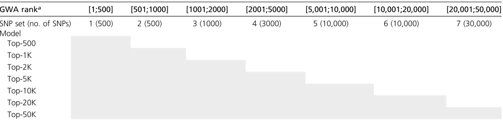
We used the results presented in Figure 1 to form SNP sets (Table 1), and with this we studied the effects of the number of markers used (p) on genomic heritability and on prediction R-sq. Both prediction R-sq. and genomic heritability esti-mates increased with the number of SNPs used (Figure 2; Supplemental Material, Figure S1 and Table S1 inFile S1) achieving values of 0.22 (95% C.I.: 0.21–0.23) and 0.45 (95% Bayesian credibility regions: 0.43–0.46), respectively. The estimated genomic heritability obtained with BayesB was very similar to those obtained with a GCTA (Table S1 inFile S1). For small SNP sets (e.g.,p= 500), the estimated genomic heritability and prediction R-sq. were similar; how-ever, while genomic heritability estimates increased steadily, the prediction R-sq. plateaued with 10K SNPs. Conse-quently, there was a widening gap between genomic herita-bility estimates and prediction R-sq. This gap can be largely attributed to the reduction in the accuracy of estimated ef-fects that takes place as the ratio between the number of SNPs (p) used in the model and sample size (n) decreases. This factor is addressed in more detail in the next section.
In Figure 2, we reported the squared correlation between predictions and adjusted phenotypes as a measure of predic-tion accuracy. The squared correlapredic-tion coincides with R2¼12½Varðy2^yÞ=VarðyÞ only when the regression of phenotypes on predictions equals one. In our study, the re-gression of phenotypes on predictions in the TST set was close to one (Table S2 inFile S1); however, there was a clear trend for the regression coefficient to become smaller than one as the number of SNPs used in the model increased.
Table 1 Grouping of SNPs into sets The shaded cells represent SNP sets included in each model.
GWA ranka [1;500] [501;1000] [1001;2000] [2001;5000] [5,001;10,000] [10,001;20,000] [20,001;50,000] SNP set (no. of SNPs) 1 (500) 2 (500) 3 (1000) 4 (3000) 5 (10,000) 6 (10,000) 7 (30,000) Model
Top-500 Top-1K Top-2K Top-5K Top-10K Top-20K Top-50K
a
Consequently, there was a small gap between the squared correlation and the traditional R2 statistic. However, this problem can be easily addressed by scaling predictions using a linear model,y¼aþb^yþe;with regression coefficients derived from a calibration set. To demonstrate this, we used 5000 records of the TST set to estimate the regression co-efficientband used the estimated coefficient to scale predic-tions. Subsequently, we used the remaining 17,221 data points of the TST set to evaluate the traditional R2and the squared correlation for the unscaledð^yÞand scaled (~y¼^b^y) predictions. After scaling, there was almost no difference be-tween the traditionalR2and the squared correlation (Table S3 inFile S1).
Forecasting the maximum prediction R-sq. that can be achieved with a SNP set
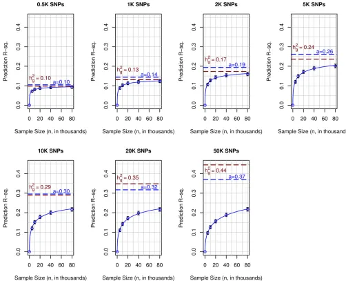
To obtain further insight on the combined effects of sample size and number of SNPs on prediction accuracy, we evaluated prediction R-sq. for predictions derived using partitions of the TRN set. For each of the SNP sets evaluated, prediction R-sq. increased with sample size (Figure 3); however, the rate of increase, and whether the curve relating prediction R-sq. with sample size reached a plateau, varied with the size of the SNP set used. For models using 500 SNPs, the prediction R-sq. increased rapidly with sample size and quickly reached a plateau with an estimated maximum prediction R-sq. of 0.1 (95% C.I.: 0.09–0.10). For models using 1K and 2K SNPs, the shape of the curve was similar to that of models using 500 SNPs; however, the maximum prediction R-sq. achieved increased with the number of SNPs used. Finally, for models using a large number of SNPs (e.g.,p$10K), the curves relating prediction R-sq. with sample size increased steadily with sample size without reaching a clear plateau.
For small SNP sets, a maximum prediction R-sq. can be safely inferred from the plots presented in Figure 3. However, for SNP sets with 10K or more SNPs, such a maximum is not
obvious. However, a simple nonlinear curve of the form R2ðniÞ ¼aðpffiffiffiffini=pffiffiffiffiffiffiffiffiffiffiffiffiffiniþbÞ þd
i (blue lines in Figure 3)fitted the observed patterns very well. The estimated asymptotic prediction R-sq. (estimated parametera;represented by the horizontal blue dashed lines in Figure 3) increased from a value of 0.1 with 500 SNPs to a value of 0.37 for panels including 50K SNPs (Figure 3). For models using up to 10K SNPs, the estimated values of parameteraand of the genomic heritability (represented by the red dashed lines in Figure 3) were very close. However, for SNP sets with 20K or more SNPs, the genomic heritability estimate was higher than the estimated maximum prediction R-sq.
The results presented above were based on SNPs selected from GWA P-values and on prediction equations estimated using model BayesB. Next, we present results obtained with alternative methods for selecting SNPs as well as different Bayesian models for estimating SNP effects.
Exploiting multi-locus LD between markers and QTL increases prediction R-sq.
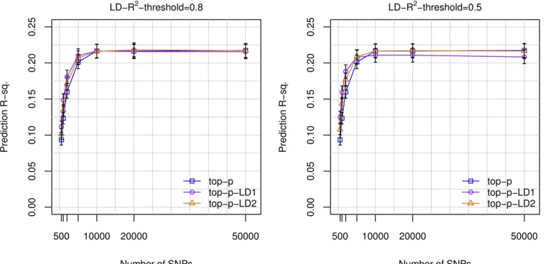
Selecting markers based on the GWAP-values can lead to the inclusion of multiple SNPs in (high) mutual LD, and this may not be optimal from a predictive perspective. To address this potential limitation, we considered constraining the selection of SNPs to either one (top-p-LD1) or two (top-p-LD2) SNPs per“LD-block.”LD-blocks were formed using LD-R2 thresh-olds of 0.8 and 0.5. For the 598,028 genotyped SNPs, those thresholds rendered a total 534,228 and 449,807 SNP sets (LD-blocks), respectively (Table S4 in File S1). For models using,10K SNPs, the top-p-LD1 and top-p-LD2 methods out-performed the top-papproach (Figure 4). However, with 10K SNPs or more, the top-p-LD1 approach was outperformed by the top-p-LD2 and top-pmethods (Figure 4).
Variable selection methods outperform shrinkage methods at high marker density
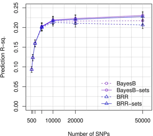
To shed light on the effect of the statistical method used on prediction R-sq., wefitted four different models (BRR, BayesB, BRR-sets, and BayesB-sets) and compared their predictive performance for varying numbers of SNPs. For models using a small number of SNPs (e.g.,p,10K), all the methods per-formed similarly (Figure 5); however, as the number of SNPs used in the model increased, the performance of these set methods (both BayesB-sets and BRR-sets) improved slightly and that of the BRR deteriorated slightly. Consequently, with 50K SNPs the set methods outperformed the prediction ac-curacy of BRR and BayesB. Using 100K SNPs (results not shown in Figure 5), model BayesB-sets achieved a prediction R-sq. of 0.24 (95% C.I.: 0.23–0.25). Inspection of estimates of regularization parameters (see Tables S5, S6, and S7 in File S1) and of estimated effects (Figure S2 inFile S1) from each of these methods shows that assigning a single Gaussian prior to all SNPs (method BRR) leads to overshrinkage of the SNPs with larger effects. This can be prevented either by using variable selection models, such as in BayesB, or with set methods.
Figure 1 Manhattan plot for human height. Results were obtained single marker least-squares regression of sex- and age-adjusted height applied to the TRN data set of 80,000 distantly related Caucasian individuals. The horizontal lines are–log10(P-value) cutoffs used to group markers into
Imputation of genotypes to higher marker density did not improve prediction R- sq.
Previous results were based on genotyped SNPs from the UK BiLEVE Axiom and the UK Biobank Axiom arrays. The max-imum prediction R-sq. that can be achieved with this set of SNPs is limited by the extent of LD between the SNPs in the array and the set of causal variants. Genotype imputation to higher SNP density can in principle lead to higher LD between markers and QTL, and this could result in higher prediction R-sq. To assess this, we repeated the analyses presented in Figure 4 using imputed genotypes (13,558,738 SNPs after quality control). The use of imputed genotypes did not lead to higher prediction R-sq. for any of the marker densities evaluated (Figure S3 and Table S8 in File S1). However, the slope of the curves relating prediction R-sq. to numbers of markers suggests that, for very large numbers of SNPs (.50K), using the high-density imputed genotypes may lead to a slightly higher prediction R-sq. than what could be achieved using genotyped SNPs. To assess this, we fitted BayesB-sets with the top-p100K SNPs chosen from the im-puted genotypes. However, the prediction R-sq. achieved in the TST set (0.20, C.I.: 0.19–0.21) was not larger than the one achieved when using 100K SNPs chosen from the geno-typed SNPs (0.24, C.I.: 0.23–0.25).
External validation in a U.S. cohort
The results presented so far were all based on independent TRN–TST sets from the UK Biobank. To assess the validity of
the prediction equations on an independent data set, we also evaluated prediction R-sq. using data from the ARIC study. Predictive ability evaluated in ARIC increased with the num-ber of SNPs used (Figure 6); however, there was a gap be-tween the prediction accuracy achieved by the same prediction equations in UK Biobank TST and ARIC. Several factors can contribute to this reduction in prediction R-sq. First, different platforms were used in ARIC and the UK Bio-bank, and the clear majority (87%) of the SNPs selected in the UK Biobank were imputed. Second, although in both cases we used data from individuals of Caucasian back-ground, there may be small differences in ethnic background between the two cohorts, with the ARIC cohort being a bit more diverse than the UK Biobank. Finally, since the two data sets originated in different countries, there may be (likely small) differences due to genetic-by-environmental interac-tion. Interestingly, the reduction in prediction R-sq. observed between the internal (UK Biobank TST) and external (ARIC) validation increased with the number of SNPs used, suggest-ing that large-effect QTL may have effects that are more sta-ble across cohorts.
Discussion
GWAS have reported large numbers of variants associated with many important complex traits and diseases. However, the proportion of variance accounted for by GWA-significant SNPs remains low; this has limited the adoption of genomic technologies in precision medicine. The relatively poor pre-diction accuracy achieved with scores based on GWA-significant SNPs has led to an increased interest in the use of WGR methods (de los Camposet al. 2010a). One line of research (Yang et al. 2010) uses WGRs (predominantly ridge regression-type methods such as G-BLUP) to estimate the proportion of variance that could be captured by regression on sets of SNPs. Empirical estimates suggest that genotyped SNPs can capture anywhere between 30 and 60% of the trait heri-tability (Yanget al.2010; Leeet al.2012; de los Camposet al. 2013b; Llewellyn et al. 2013). More recently, studies using rare and common variants suggest that the amount of var-iance that could be captured by regression on SNPs could be even higher, approaching the trait heritability (Yang et al. 2015). However, as argued by Makowsky et al. (2011), these results do not necessarily reflect the ability of a model to predict future outcomes. Unfortunately, the few studies that (until recently) have used G-BLUP-type methods for prediction of complex traits using distantly related individ-uals (de los Camposet al.2013b) were based on relatively small training data sets. Consequently, the prediction R-sq. reported were not considerably higher than what can be obtained using genetic scores based on GWAS-significant SNPs (de los Camposet al.2013b). Better results have been obtained using family data (de los Campos et al. 2012; Vazquez et al. 2012); however, as noted by the authors, these results pertain to“family-based”risk prediction and are not applicable in the general population (Makowsky
et al.2011; Vazquezet al.2012, 2016; de los Camposet al. 2013b).
The main explanation for the relatively disappointing pre-diction accuracy achieved with WGR methods in prepre-diction of disease risk with unrelated individuals has been that the number of SNP effects that need to be estimated is usually large relative to sample size. This leads to low accuracy of estimated effects and consequently to a widening gap between the genomic heritability and prediction R-sq. In principle, the use of big data should lead to a substantial reduction of the gap between prediction R-sq. and the trait heritability. Our results support this hypothesis.
Using 80K records for model training and top-100K GWAS-selected SNPs, we were able to achieve a prediction R-sq. of 0.24 (95% C.I.: 0.23–0.25, model BayesB-sets). This repre-sents approximately one-third of the trait heritability. The
Genetic Investigation of ANthropometric Traits (GIANT) con-sortium reported an R-sq. of 0.17 using 2K SNPs selected based on GWAS meta-analysis (n= 253,288) (Wood et al. 2014). For the same number of SNPs, we obtained a similar prediction R-sq. (0.16, Table S9 inFile S1). However, we also observed that higher prediction R-sq. can be achieved using more SNPs (up to 0.24 with 100K SNPs).
Canela-Xandri et al.(2016) also used data from the in-terim release of the UK Biobank to assess prediction accu-racy of human height using a G-BLUP (a model similar to the BRR used here). Usingp= 319,038 common SNPs (MAF. 0.05) andn= 114,264 individuals for model training, they achieved a prediction correlation of 0.53 (a squared correla-tion of 0.28) on a testing set ofn= 9583 white Caucasians individuals. This value is higher than what we reported here for model BayesB-sets withp= 100K SNPs (0.24). However,
Figure 3 Polygenic prediction coupled with big data closes a sizable fraction of gap between prediction R-sq. and trait heritability. Each panel shows the average prediction R-sq. (s) achieved in the testing set (n= 22,221) by the number of SNPs used (p= 500, 1K,⋯;50K,K= 1000)vs.the size of the data set used to train models. The solid blue curve corresponds to a nonlinear function,R2ðnÞ ¼apnffiffiffi=pffiffiffinþb; fitted by least squares. The dashed blue
the two studies are not strictly comparable due to two main reasons. First, the TST set used in our study (n= 22,221) included individuals that were distantly related to those used for TRN (all TRN–TST genomic relationships satisfied Gij,0.03); therefore, our TRN and TST sets were distantly related. On the other hand, in Canela-Xandri et al.(2016), the individuals used for validation had at least one genomic relationship .0.0625 with the individuals used for model training; therefore, in the study Canela-Xandriet al., individ-ual in the training and testing set were not as distantly related as in our study. Second, our training size was 30% smaller (nTRN = 80K compared withn= 114,264). However, de-spite the differences in the size of the TRN set and the rela-tionships between TRN and TST sets, the two studies suggest that using a training size of the order of 100K subjects can lead to a prediction R-sq. for human height of30–35% of the trait heritability.
Even for traits affected by large numbers of small-effect loci, a sizable fraction of the SNPs available in a modern SNP array is likely to be in weak or no LD with QTL. Removing SNPs that are in linkage equilibrium with QTL should not reduce genomic heritability and can lead to more accurate estimates of effects; therefore, as previously shown in other studies (Lango Allen et al. 2010), preselection of SNPs can be an effective strategy when deriving equations for prediction of complex human traits. However,how many SNPs should be used? Our study shows that, because of the tradeoff existing between genomic heritability and the accuracy of estimated effects, this question does not have a universal answer. For example, for TRN data sets withn= 5K samples or fewer, the maximum prediction R-sq. was achieved withp= 5K SNPs (Figure S1 in File S1); however, for models trained with larger sample sizes (e.g.,n= 80K), the prediction R-sq. con-tinued to increase as more SNPs were added to the model, reaching a plateau with10K SNPs (e.g., with model BayesB, see Figure S1 inFile S1).
Thestatistical model used to estimate effectshas received a great deal of attention in both the animal and plant genomic literature (Gianola et al. 2009; Habier et al. 2011; de los Campos et al. 2013a; Wimmer et al. 2013). However, this has not been the case in human genetics where most of the WGR studies published are based on shrinkage methods. This is rather surprising considering that variable selection is po-tentially more relevant when LD spans over short regions; a situation that is more likely in human genomes than in those from breeding populations. We compared shrinkage and vari-able selection methods and, overall, did notfind very large differences between methods. However, this is partially a consequence of (i) the complexity of the trait analyzed (hu-man height), which is characterized by having large numbers of small effects loci; and (ii) the use GWA-selected SNPs (by preselecting SNPs, large numbers of the SNPs with no effects are removed in thefirst step). In this setting, and when the number of SNPs selected is moderate (e.g.,p#2K), different estimation methods lead to very similar prediction R-sq. However, when using large numbers of SNPs (e.g., p $ 10K), we observed that models based on a single normal distribution of effects (BRR) led to overshrinkage of the esti-mates of large-effect variants (Figure S2 inFile S1) and to lower prediction R-sq. (Figure 5). Therefore, whenpis large, it seems clear that either using variable selection methods (e.g., BayesB) or grouping SNPs into sets according to some proxy of the size of their effects (as done here in BRR-sets and BayesB-sets) can lead to higher prediction R-sq.
In this study, we have focused on additive models where SNPs enter linearly in the prediction equation and are as-sumed to be the same for all individuals. For some traits and diseases, it is possible that higher prediction accuracy could be achieved by accounting for nonadditive effects (e.g., domi-nance, epistasis). In high-dimensional models, epistasis could be captured using semiparametric methods such as kernel regressions (e.g., de los Camposet al.2010b). However, for
Figure 4 Prediction R-sq. achieved vs. number of SNPs used in the model, by marker selection strat-egy. Prediction R-sq. achieved in the UK Biobank TST set (n = 22,221) obtained with models
fitted using a training data set of 80,000 subjectsvs.the number of SNPs used. BayesB models were
fitted using genotyped SNPs and three different strategies for SNP selection: top-pincludes thepSNPs with the smallest GWA P-value, top-p-LD1 and top-p-LD2 select the pSNPs with smallest GWA P-value (derived from the TRN set) subject to the restriction of choos-ing only one or two SNPs per LD-block, respectively. LD-blocks were determined using an LD-R2
many traits and diseases, including anthropometric traits such as human height, the gap between the broad and the narrow sense heritability (Falconer and Mackay 1996) is small. In such cases, the potential to improve prediction accuracy by accounting for nonadditive effects is limited. Likewise, for some traits and diseases, incorporating genetic-by-environmental interactions could be an avenue to further improve prediction accuracy. However, this is unlikely the case for prediction of human stature of individuals without nutritional deprivation.
In recent years, there has been an important debate as to whether and how to deal with near collinearity (a phenom-enon that can emerge when using multiple markers in high LD) in genomic analysis of complex traits. This debate has been largely centered on the problem of estimating genomic heritability (Gianolaet al.2009; de los Camposet al.2013b). Here, we approach the problem from a predictive perspective by comparing methods that use either one or two SNPs per LD block with a method that selects SNPs based on GWA P-values irrespective of the LD structure. The latter approach leads to the selection of multiple markers per LD block. When a small number (e.g.,p= 500) of SNPs was used, the top-p-LD1 method was better than the method using the top-p SNPs. This happens because when only a few SNPs are used, the SNPs selected by the top-p method clustered in a few regions and did not provide a good coverage of the genome. This can be avoided by choosing only one or two SNPs per LD block. However, for prediction equations based on a larger number of SNPs (e.g.,p$10K) the methods that used
mul-tiple markers per LD block (either top-p-LD2 or top-p) out-performed the top-p-LD1 method, suggesting that exploiting multi-locus LD between markers and QTL is needed to achieve higher prediction R-sq. This seems to be an instance where the realms of inference (e.g., estimation of genomic heritability) and prediction needs to be distinguished: high LD between predictors can lead to problems for inferences about variances and about individual marker effects; how-ever, multi-locus LD seems to be an important feature to be exploited when it comes to prediction.
Previous studies suggest that the use of genotypes imputed to high marker density (e.g.,17 million) (Yanget al.2015) can lead to estimates of genomic heritability considerably higher than those obtained with common SNPs. However, in our studymodels based on imputed genotypesdid not yield higher prediction R-sq. than those based on genotyped SNPs. When only a small number of variants (e.g.,p= 1K) were used, the prediction R-sq. of models based on genotyped SNPs was higher than the one obtained when those SNPs were selected from both genotyped and imputed SNPs. With higher marker density (e.g., models withp= 100K), models based on genotyped and imputed SNPs performed similarly. The UK Biobank also provides data from non-Caucasian subjects. When we used the prediction equations derived from the TRN set to predict individuals of other ethnic backgrounds, we observed a substantial reduction in prediction R-sq. (Fig-ure S4 inFile S1). The additive effects of SNPs can depend on both allele frequencies and LD patterns (de los Camposet al. 2015b; Lehermeier et al. 2015). These two features of ge-nomes are likely to vary between populations, making linear models such as the one considered here useful within the population that was used to estimate effects. Interestingly, the gap between the within- and across-ethnic group predic-tion R-sq. increased as the number of SNPs included in the
Figure 6 An external validation in a U.S. cohort yields moderately high prediction R-sq. Each bar shows the prediction R-sq. by combinations of genotypes and numbers of SNPs in ARIC (nTST = 9591) and UK Biobank (nTST = 22,221) cohorts. The vertical bars represent 95% C.I.’s. UKB, UK Biobank.
model grew from 500 to 50K. This suggests that the extent of effect heterogeneity between populations is likely to be smaller for large-effect variants and larger for variants with small ef-fects. The vast majority of the GWA data collected in the last two decades originates from individuals of Caucasian origin (Bustamante et al.2011; Popejoy and Fullerton 2016). The results reported here fortrans-ethnic prediction highlight the importance of further investing in the collection of large data sets for non-Caucasian individuals.
Conclusion
Will big data close the missing heritability gap? Our results indicate that even for a highly complex trait such as standing height, the use of polygenic prediction coupled with big data can close a sizable fraction of the gap between trait heritability and prediction R-sq. With a TRN size of 80K records we were able to achieve a prediction R-sq. of about one-third of the trait heritability.
Soon, much larger data sets with several hundreds of thou-sands of individual phenotype–genotype records will become available. Forecasting prediction R-sq. for such data sets implies extrapolating beyond the sample size considered here and is a question that can only be answered once such data sets become available. However, thefitted response curves (Figure 3) suggest that, for the top-50K SNPs identified in this study, the (esti-mated) maximum prediction R-sq. that could be achieved is 0.37. These forecasts pertain to the set of 50K SNPs that was selected using GWAP-values derived from a training set of 80K samples. If one had access to 1 million records, the GWAS would be more accurate and this would likely lead to the selection of a better 50K SNP set than the one selected here. Moreover, with 1 million records it is likely that models using.50K will out-perform those based on the top-50K SNPs. Therefore, we con-clude that the advent of big data will lead to a sizable improvement of our ability to predict complex human traits and diseases. This can make genomic prediction of many mod-erately heritable traits and diseases practically useful.
Acknowledgments
The authors thank the participants and the personnel in charge of generating, curating, and maintaining the data of the UK Biobank and Atherosclerosis Risk in Communities studies, and Dr. Kyle Grimes for helping us on improving the quality of our manuscript. G.d.l.C., A.I.V., H.K., and A.G. had financial support from National Institutes of Health grants R01 GM-099992 and R01 GM-101219. This work was supported in part by Michigan State University through computational resources provided by the Institute for Cyber-Enabled Research.
Literature Cited
Allen, N. E., C. Sudlow, T. Peakman, and R. Collins; UK Biobank, 2014 UK biobank data: come and get it. Sci. Transl. Med. 6: 224ed4.
Bustamante, C. D., E. G. Burchard, and F. M. De La Vega, 2011 Genomics for the world. Nature 475: 163–165. Canela-Xandri, O., K. Rawlik, J. A. Woolliams, and A. Tenesa,
2016 Improved genetic profiling of anthropometric traits us-ing a big data approach. PLoS One 11: 1–12.
Chang, C. C., C. C. Chow, L. C. Tellier, S. Vattikuti, S. M. Purcell et al., 2015 Second-generation PLINK: rising to the challenge of larger and richer datasets. Gigascience 4: 7.
Collins, F. S., and H. Varmus, 2015 A new initiative on precision medicine. N. Engl. J. Med. 372: 793–795.
Daetwyler, H. D., B. Villanueva, and J. A. Woolliams, 2008 Accuracy of predicting the genetic risk of disease using a genome-wide ap-proach. PLoS One 3: e3395.
de los Campos, G., D. Gianola, and D. B. Allison, 2010a Predicting genetic predisposition in humans: the promise of whole-genome markers. Nat. Rev. Genet. 11: 880–886.
de los Campos, G., D. Gianola, G. J. M. Rosa, K. A. Weigel, and J. Crossa, 2010b Semi-parametric genomic-enabled prediction of genetic values using reproducing kernel Hilbert spaces methods. Genet. Res. 92: 295–308.
de los Campos, G., Y. C. Klimentidis, A. I. Vazquez, and D. B. Allison, 2012 Prediction of expected years of life using whole-genome markers. PLoS One 7: e40964.
de los Campos, G., J. M. Hickey, R. Pong-Wong, H. D. Daetwyler, and M. P. L. Calus, 2013a Whole-genome regression and pre-diction methods applied to plant and animal breeding. Genetics 193: 327–345.
de los Campos, G., A. I. Vazquez, R. Fernando, Y. C. Klimentidis, and D. Sorensen, 2013b Prediction of complex human traits using the genomic best linear unbiased predictor. PLoS Genet. 9: e1003608.
de los Campos, G., D. Sorensen, and D. Gianola, 2015a Genomic heritability: what is it? PLoS Genet. 11: e1005048.
de los Campos, G., Y. Veturi, A. I. Vazquez, C. Lehermeier, and P. Pérez-Rodríguez, 2015b Incorporating genetic heterogeneity in whole-genome regressions using interactions. J. Agric. Biol. Environ. Stat. 20: 467–490.
Erbe, M., B. Gredler, F. R. Seefried, B. Bapst, and H. Simianer, 2013 A function accounting for training set size and marker density to model the average accuracy of genomic prediction. PLoS One 8: e81046.
Falconer, D. S., and T. F. C. Mackay, 1996 Introduction to quanti-tative genetics, Ed. 4. Longmans Green, Harlow, UK.
Gaziano, J. M., J. Concato, M. Brophy, L. Fiore, S. Pyarajanet al., 2016 Million veteran program: a mega-biobank to study ge-netic influences on health and disease. J. Clin. Epidemiol. 70: 214–223.
Gianola, D., G. de los Campos, W. G. Hill, E. Manfredi, and R. Fernando, 2009 Additive genetic variability and the Bayesian alphabet. Genetics 183: 347–363.
Goddard, M., 2009 Genomic selection: prediction of accuracy and maximisation of long term response. Genetica 136: 245–257. Goddard, M. E., B. J. Hayes, and T. H. E. Meuwissen, 2011 Using
the genomic relationship matrix to predict the accuracy of ge-nomic selection. J. Anim. Breed. Genet. 128: 409–421. Habier, D., R. L. Fernando, K. Kizilkaya, and D. J. Garrick,
2011 Extension of the bayesian alphabet for genomic selec-tion. BMC Bioinformatics 12: 186.
Lango Allen, H., K. Estrada, G. Lettre, S. I. Berndt, M. N. Weedon et al., 2010 Hundreds of variants clustered in genomic loci and biological pathways affect human height. Nature 467: 832–838.
Lehermeier, C., C.C. Schön, and G. de los Campos, 2015 Assessment of genetic heterogeneity in structured plant populations using multivariate whole-genome regression models. Genetics 201: 323–337.
Lehermeier, C., G. de los Campos, V. Wimmer, and C. C. Schön, 2017 Genomic variance estimates: with or without disequilib-rium covariances? J. Anim. Breed. Genet. 134: 232–241. Llewellyn, C. H., M. Trzaskowski, R. Plomin, and J. Wardle,
2013 Finding the missing heritability in pediatric obesity: the contribution of genome-wide complex trait analysis. Int. J. Obes. 37: 1506–1509.
Maher, B., 2008 Personal genomes: the case of the missing heri-tability. Nature 456: 18–21.
Mailman, M., M. Feolo, Y. Jin, M. Kimura, K. Tryka et al., 2007 The NCBI dbGaP database of genotypes and phenotypes. Nature 39: 1181–1186.
Makowsky, R., N. M. Pajewski, Y. C. Klimentidis, A. I. Vazquez, C. W. Duarteet al., 2011 Beyond missing heritability: Prediction of complex traits. PLoS Genet. 7: e1002051.
Manolio, T. A., F. S. Collins, N. J. Cox, D. B. Goldstein, L. A. Hindorff et al., 2009 Finding the missing heritability of complex diseases. Nature 461: 747–753.
Meuwissen, T. H. E., B. J. Hayes, and M. E. Goddard, 2001 Prediction of total genetic value using genome-wide dense marker maps. Genetics 157: 1819–1829.
O’Connell, J., K. Sharp, N. Shrine, L. Wain, I. Hall et al., 2016 Haplotype estimation for biobank-scale data sets. Nat. Genet. 48: 817–820.
Pérez, P., and G. de los Campos, 2014 Genome-wide regression and prediction with the BGLR statistical package. Genetics 198: 483–495.
Popejoy, A. B., and S. M. Fullerton, 2016 Genomics is failing on diversity Alice. Nature 538: 161–164.
Ripke, S., B. M. Neale, A. Corvin, J. T. R. Walters, K.-H. Farhet al., 2014 Biological insights from 108 schizophrenia-associated genetic loci. Nature 511: 421–427.
Speliotes, E. K., C. J. Willer, S. I. Berndt, K. L. Monda, G. Thorleifsson et al., 2010 Association analyses of 249,796 individuals reveal 18 new loci associated with body mass index. Nat. Genet. 42: 937–948.
The SIGMA Type 2 Diabetes Consortium, A. L. Williams, S. B. Jacobs, H. Moreno-Macías, A. Huerta-Chagoyaet al., 2014 Sequence var-iants in SLC16A11 are a common risk factor for type 2 diabetes in Mexico. Nature 506: 97–101.
UK Biobank, 2007 UK Biobank: protocol for a large-scale prospec-tive epidemiological resource, pp. 1–112. Accessed May 7, 2016.
Available at: http://www.ukbiobank.ac.uk/wp-content/uploads/ 2011/11/UK-Biobank-Protocol.pdf.
UK Biobank, 2015 Genotyping and quality control of UK Biobank, a large-scale, extensively phenotyped prospective resource, pp. 1–27. Accessed May 7, 2016. Available at:https://biobank.ctsu. ox.ac.uk/crystal/docs/genotyping_qc.pdf.
Vazquez, A. I., G. J. M. Rosa, K. A. Weigel, G. de los Campos, D. Gianolaet al., 2010 Predictive ability of subsets of single nu-cleotide polymorphisms with and without parent average in US Holsteins. J. Dairy Sci. 93: 5942–5949.
Vazquez, A. I., G. de los Campos, Y. C. Klimentidis, G. J. M. Rosa, D. Gianola et al., 2012 A comprehensive genetic approach for improving prediction of skin cancer risk in humans. Genetics 192: 1493–1502.
Vazquez, A. I., Y. Veturi, M. Behring, S. Shrestha, M. Kirst et al., 2016 Increased proportion of variance explained and pre-diction accuracy of survival of breast cancer patients with use of whole-genome multiomic profiles. Genetics 203: 1425–1438.
Voight, B. F., L. J. Scott, V. Steinthorsdottir, A. P. Morris, C. Dina et al., 2010 Twelve type 2 diabetes susceptibility loci identified through large-scale association analysis. Nat. Genet. 42: 579– 589.
Wall, J. D., and J. K. Pritchard, 2003 Haplotype blocks and link-age disequilibrium in the human genome. Nat. Rev. Genet. 4: 587–597.
Wimmer, V., C. Lehermeier, T. Albrecht, H. J. Auinger, Y. Wang et al., 2013 Genome-wide prediction of traits with different genetic architecture through efficient variable selection. Genet-ics 195: 573–587.
Wood, A. R., T. Esko, J. Yang, S. Vedantam, T. H. Pers et al., 2014 Defining the role of common variation in the genomic and biological architecture of adult human height. Nat. Genet. 46: 1173–1186.
Yang, J., B. Benyamin, B. P. McEvoy, S. Gordon, A. K. Henderset al., 2010 Common SNPs explain a large proportion of the herita-bility for human height. Nat. Genet. 42: 565–569.
Yang, J., S. H. Lee, M. E. Goddard, and P. M. Visscher, 2011 GCTA: a tool for genome-wide complex trait analysis. Am. J. Hum. Genet. 88: 76–82.
Yang, J., A. Bakshi, Z. Zhu, G. Hemani, A. A. E. Vinkhuyzenet al., 2015 Genetic variance estimation with imputed variantsfinds negligible missing heritability for human height and body mass index. Nat. Genet. 47: 1114–1120.