High Order Finite Elements in Free Vibrations of Thick Plates

(1)

18th International Conference on Structural Mechanics in Reactor Technology (SMiRT 18) Beijing, China, August 7-12, 2005 SMiRT18-B04-7

HIGH ORDER FINITE ELEMENTS IN FREE VIBRATIONS OF THICK

PLATES

S.F.SILVA

Universidade de Brasília – Faculdade de

Tecnologia – Departamento de

Engenharia Civil - Cx.Post 04492

Phone: 0055 3072325,

Fax: 0055 2734644

E-mail: seleniofeio@unb.br

L.J.Pedroso

Universidade de Brasília – Faculdade de

Tecnologia – Departamento de

Engenharia Civil - Cx.Post 04492

Phone: 0055 3072325,

Fax: 0055 2734644

E-mail:

lineu@unb.br

ABSTRACT

The aim of this paper is to study the dynamic behavior of plates through the Reissner-Mindlin’s theory, making use of the Finite Elements Technique to solve the displacement equation of plates in free vibration. The finite element adopted is the Lagrangean quadrangular of sixteen nodes (QL-16). In the first numerical example the criterion of Hinton & Huang’s (1986) for discretization of circular plates is applied. In order to reproduce experimental results obtained by Pedroso (1983,1986), with a circular plate of steel and another of rubber both fixed with bolts, different boundary conditions are tested. In the second numerical example, the same discretization criterion is used for elliptical plates with different eccentricities. This time the finite element QL-16 is tested in several deformed shapes in order to observe the behavior of the solution.

Keywords: High order finite elements, theory of Reissner-Mindlin, dinamic of thick plates.

1. INTRODUCTION

Theory of plates can be applied on design of several engineering structures, such as bridge decks, tracking systems, retaining walls, water tanks, ships' hulls, car parts, spacecrafts, nuclear reactors, among others.

Basically, plate theories vary according to the hypothesis regarding rotation of normal to the midplane. Hence according to the classical theory of Kirchhoff’s for thin plates, these normals remain straight and orthogonal to the deformed midplane, (Timoshenko, 1970; and Szilard, 1974). Normals in theories such as Reissner-Mindlin, however, must still remain straight but not necessarily orthogonal do the deformed midlplane (Reissner, 1945; and Mindlin, 1951).

Plate elements based on Kirchhoff theory are used only on thin plates (thickness / width ≤ 0.10), but it is difficult to find shape functions that meet requirements of displacement and deflection continuity throughout this element. An alternative formulation, based on Reissner-Mindlin’s theory of plates, can be applied to thin and thick plates and also helps to avoid the limitations regarding Kirchhoff’s elements. On this account, Reissner-Mindlin’s theory of thin plates is here adopted.

Under certain geometrical, binding and loading conditions Kirchhoff’s plates have analytical solutions, being some of which very work demanding. Examples of such analytical solutions to obtain natural frequencies of Kirchhoff’s plates are presented in the work of Leissa (1971). In the case of Reissner-Mindlin’s plate, analytical solutions are almost non-existent due to the high complexity level of the equations.

(2)

of plate.

Although QL-16 is considered an element of high order, it doesn´t necessarily increase the computational costs, because meshes can be less refined. It also presents better results compared to lower order elements (Silva, 1998).

Finite elements based on Reissner-Mindlin’s theory are in general unable to reproduce the thin plate condition, causing the so called “solution-locking effect”. In the QL-16 element, adopted in this paper, this effect is not observed. This is one of the advantages of the QL-16 over the low order elements, that need the use of imposed shear or a reduced integration technique to avoid solution-locking effect.

Further details regarding plate bending can be found, for example, in Bathe & Dvorkin (1985), Hinton & Huang (1986), in Zienkiewicz & Taylor (1991), Oñate (1995) and Silva (1998).

2. THE FINITE ELEMENT METHOD APPLIED TO REISSNER-MINDLIN’S THEORY

In dynamic problems the displacements, velocities, deformations, tensions and loading are all time dependent. The procedure of general equation derivation by finite elements to a dynamic problem can be obtained through the following steps:

1º - A body is idealized in E finite elements;

2º - A displacement model is assumed for element E.;

[

]

u

( , , , )

Q

( , , , )

( , , )

( )

x y z t

u x y z t

v x y z t

w x y z t

x y z

e

t

=





















=

Φ

(1)

where

u

the displacement vector,

Φ

is the matrix of form functions, so that

Q

is the vector of nodal displacements which is assumed to be a function of time t;

( )e

3º- the element characteristic of the matrixes of stiffness, of mass and of the characteristic vector of charge is derived.

From equation (1), the deformation can be expressed as,

ε =

B Q

( )e (2)

and the tensions as,

) (e

Q

B

D

=

ε

σ

(3)

Unlike equation (1) in relation to time, the velocity field can be obtained through,

&

( , , , )

[ ( , , )]

&

( )

u

x y z t

= Φ

x y z

Q

e

t

(4)

where is the nodal velocities vector. To derive the equation of movement of the structure, Lagrange’s Equations or Hamilton’s Principle can be used. Lagrange’s equations are given by;

&

( )

Q

e

{ }

d

dt

L

R

∂

&

Q













− 









+













=

0

(5)

where,

L

= − π

C

_P (6)

is called the Lagrangean function, C is the kinetic energy, πP is the potential energy, R is the dissipation function, Q is the nodal displacement and

Q

&

is the nodal velocity.

The kinetic and potential energy for “e” can be written as,

C

e T

d

V e ( )

( )

& &

=

1 _∫∫∫

2 ρ

u u

V

(7)

π

_Pe T T T

V e A e

V e

dV

dA

dV

( )

( ) ( )

( )

=

1 _∫∫∫

−

_∫∫

_{− ∫∫∫}

2 ε σ

u

Λ

u

Λ

(8)

(3)

R

e T

d

V e

( )

& &

=

1 _∫∫∫

2 µ

u u

V

(9)

where µ is called the damping coefficient. In equations (7) to (9), the integral volume has to be made over the volume of the element and in equation (8), the integral surface has to be made over part of the element surface where the overall surface forces are known. Using the equations (1) to (3), the expression for C, πP and R can be

written as:

C

e

dV

e E

T T

V e e

E

= ∑

=



∑

∫∫∫











= =

( )

&

[ ] [ ]

&

1 1

1

2 Q

ρ Φ

Φ

Q

(10)

π

_P

π

e E

T T

V e e

E

T T

A e e

E

T

V e

T C

dV

t dA

t dV

t

= ∑

=



∑

_∫∫∫











−



∑

∫∫

+ ∫∫∫







_

 −

= =

= P (e)

1 1

1

2 Q

B

D B

Q

[ ] [ ] [ ]

[ ]

( )

[ ]

( )

( ) ( )

Φ Λ

P

(11)

R

e

dV

e E

T T

V e e

E

= ∑

=



∑

∫∫∫











= =

( )

&

[ ] [ ]

&

1 1

1

2 Q

µ Φ

Φ

Q

(12)

where

Q

is the nodal global displacement vector,

Q

&

is the nodal global velocity vector, and

P

is the nodal concentrated loadvector for the structure.

C

The matrixes involved in the integrals are defined as,

[M(e)] = element mass matrix =

ρ

[ ] [ ]

( )

Φ

T

Φ

V e

dV

∫∫∫

₍₁₃₎

[K(e)] = element stiffness matrix =

[ ] [ ] [ ]

( )

B

T

D B

V e

dV

∫∫∫

₍₁₄₎

[ζ(e)] = element damping matrix =

µ

[ ] [ ]

( )

Φ

T

Φ

V e

dV

∫∫∫

₍₁₅₎

[PS(e)] = nodal forces element of the vector produced by the surface forces =

[ ]

( )

Φ Λ

T

A e

dA

∫∫

₍₁₆₎

[Pb(e)] = nodal forces element of the vector produced by the body forces =

[ ]

( )

Φ Λ

T

V e

dV

∫∫∫

₍₁₇₎

4º- Element matrixes and vectors are constructed and the general displacement equations system is derived.

The equations (10) to (12) can be written as:

C

=

1

T

2 Q

&

[

M Q

]

&

(18)

π

_P

₌

1

T

₋

T

2 Q

[

K Q

]

Q P

(19)

R

=

1

T

(4)

]

where, [M] = structure mass matrix = ; [K] = structure stiffness matrix = ; [ζ] = structure

damping matrix = ;

[

M

( )e

e E

=

∑

1

[

K

( )e

e E

=

∑

1

[

ζ

( )e

]

e

E

=

∑

1

P

_(t) = total loading vector =

(

P

_Se

P

_be

)

e E

t

( ) ( )

( )

∑

=1

+

P

C

( )

t

.

Substituting the equations (18) to (20) on equation (5), the structure displacement equation is obtained:

[

M Q

]

&&

( )

t

+

[ ]

ζ

Q

&

( )

t

+

[ ]

K Q

( )

t

=

P

_{( )}_C

( )

t

(21)

where

Q

&&

is the nodal acceleration vector in the global system. If damping is ignored, the displacement equation can be written as,

[

M Q

]

&&

( )

t

+

[ ]

K Q

( )

t

=

P

_{( )}_C

( )

t

(22)

5º e 6º- The displacement equation is solved.

From equation (7), substituting the values of BT D B:

B D BT

i i i i i i i i f f f f f c c j j j j j j j j x y x y y x D D D D MD D D x y y x x y = − − − − − −                                   − − − − − − − −                    

0 0 0

0 0

0 0 0

0 0 0 0

0 0 0 0 0 0 0 ∂φ ∂ ∂φ ∂ ∂φ ∂ φ ∂φ ∂ ∂φ ∂ φ ν ν ∂φ ∂ ∂φ ∂ ∂φ ∂ ∂φ ∂ ∂φ ∂ φ ∂φ ∂ φ ∂φ ∂           (23)

Multiplying the expression (23):

D

x x D y y D x D y

D

x D D x x MD y y MD x y D x y

D

y MD x y D x y D D y y MD x x

c i

j

c i

j

c j i c j i

c i

j

c i j f i

j f i j f j i f i j c i j f i j f j i

c i j f i

j f i j ∂φ ∂ ∂φ ∂ ∂φ ∂ ∂φ ∂ φ ∂φ ∂ φ ∂φ ∂ φ ∂φ ∂ φ φ ∂φ ∂ ∂φ ∂ ∂φ ∂ ∂φ ∂ ∂φ ∂ ∂φ ∂ ν ∂φ ∂ ∂φ ∂ φ ∂φ ∂ ∂φ ∂ ∂φ ∂ ν ∂φ ∂ ∂φ ∂ φ φ ∂φ ∂ ∂φ ∂ ∂φ ∂ ∂φ ∂ + − − − + + + − + +                   + (24) where, 2 1 ; ) 1 ( 12 ; ) 1 ( 12 5 2 3 _ν ν ν − = − = +

= hE D Eh M

D_c _f

ν: Poisson’s ratios;

E : Young’s modulus;

D

_f : Flexural rigidity of the plate;

D

_c : Shearing rigidity of the plate;

M : Constitutive matrix of the plate;

φi : Shape functions of QL16 element;

∂φ ∂

_i

x

: Derivative of shape functions in the x direction;

∂φ ∂

_i

y

: Derivative of shape functions in the y direction.

(5)

1 5 6 2

12 13 14 7

11 16 15 8

4 10 9 3

x y

(

w,θ θ_x, _y

)

T

(ξ) (η)

Figure 1-a. Lagrangean Quadrilateral Element of 16 Nodes.

1

5 6

2 12

13 14

7 11

16 15

8 4

10 9

3

x y

z

Figure 1-b. Degrees of freedom in the Lagrangean Quadrilateral Element of 16 Nodes.

Figure 1. Diagram and Freedom Degrees in the Lagrangean Quadrilateral Element of 16 Nodes.

7

18 17 16 15 14 13 1

2

3

39 38 37

42 41 40

21 20 19

6 4

5 45 44 43 48 47 46 33 32 31

36 34

35

30 29 28 12 11 10

24 22

23 25

27 26

8

9

The mass matrix for each node of the element (QL-16) is, therefore, 3x3 and can be written (Karunasena, Liew and Al-Bermani, 1996) as:

M

_no

cc cd ce dd de

ee _x

M

′

=













3 3

(25)

onde:

M

_cc T

J dv

M

_cd

M

_ce v

=

_{∫ Φ Φ ρ}

;

=

0 ;

=

0

₍₂₆₎

M

_dd

h

_x _xT

J dv

M

_de v

=

_∫

=

12 Φ Φ ρ

;

0

(27)

M

_ee

h

_y _yT

J dv

v

=

_∫

12 Φ Φ ρ

(28)

; ρ is the material mass for each volume unit and h is plate thickness, Φ represents the element shape function and

| J | the Jacobian.

The elementary mass matrix for the element (QL-16) has order 48x48(number of nodes in the element x freedom degrees for each node). Considering the material to be isotropic (ρ = cte) and knowing that | J | = A/4

(Jacobian rectangular element, that allows to express the differential of the field in natural coordinates), it can be written, respectively, as the translational element and as the elementary mass matrix element:

∫ ∫

+

− +

−

=

1

1 1

1

4 φ

φ

η

ξ

ρ

A

h

d

m

i j

TRANSL.

ij (29)

∫ ∫

+

− +

−

=

1

1 1

1 3

48 φ

φ

η

ξ

ρ

A

h

d

m

i j

ROTAC.

(6)

3. RESULTS

Two cases concerning the dynamic analysis of plates are presented, in order to assess the potentiality of the element here adopted, in specific situations. Circular and eliptical plates were analysed to verify the behaviour of the deformed element QL-16.

The results were compared to analytical solutions of kirchhoff’s models (Szilard, 1974), and Dawe & Roufaeil

(1980) and to experimental results (Pedroso, 1983 and 1986).

Case 1

In this case the dynamic behaviour of two vibrating plates is studied, one made of steel and the other made of rubber. The boundary conditions in these two plates, as well as the characteristics of the materials, steel and rubber, are displayed in Table 1-a.

Tabela 1-a. Real support conditions on the plate and material characteristics.

REAL SUPPORT CONDITIONS MATERIAL OF THE PLATES

4

3

2

1 5

6

7

8

STEEL:

E = 2.06 x 1011 N / m2

ρ = 7970 Kg / m3

ν = 0.29

r0 = 0.0425 m

m = 0.023 Kg

S = 0.0057 m2

h = 0.0005 m

RUBBER:

E = 1 x 108N / m2

ρ = 1500 Kg / m3

ν = 0.45

r0 = 0.0425 m

m = 0.0255 Kg

S = 0.0057 m2

h = 0.003 m

The bond of the plate is obtained through screws (bolts). The materials transversal elasticity mode is E, ρ is the volumetric mass, ν is the Poisson coefficient, r0 is the plate radius, m is the plate mass, S is the area on the circular platesurface and h is the thickness of the plate.

Considered as an exact result for the two vibrating membranes, mentioned above, the experimental values of the fundamental frequencies found by Pedroso (1983 and 1986), for steel and rubber plates, respectively: f11aço =

210 Hz e f11bor = 110 Hz.

(7)

Table 1-b. Types of boundary conditons used on vibrating membranes. FREQUENCIES (Hz)

TYPES BOUNDARY STEEL RUBBER

CONDITIONS USED ANALYTICAL NUMERICAL ANALYTICAL NUMERICAL

TYPE 01: campled

690 691 225 222

TYPE 02: supported

336 333 110 113

TYPE 03: three bolts

--- 230 --- ---

TYPE 04: six bolts

--- --- --- 108

It is observed that the numerical mode of Type 03 (three bolts - 1200) is the one that best represents the steel bladeexperiment, for the rubber blade modeling, both analytical and numerical, which consider the blade to be totally supported (Type 02) are the ones that best represent the experiment. As for the case of the rubber blade, the numerical mode of Type 04 (six bolts - 600) also represents well the experiment.

Case 2:

This example consists of the use of element QL-16 in totally clamped elliptical plates. Through the concept of eccentricity of (e = b/a), where e represents the eccentricity of the ellipse, b the smallest radium and a the largest radium, five elliptical clamped plates, each one with its respective eccentricity and discretization in twelve elements QL-16 (Figure 2).

The parameter to be compared is

λ ω

(

)

, where ω is the fundamental circular frequency, a

represents the largest radius, the ma is the thickness of the plate and D is the stiffness of the elliptical plate, (

ρ

=

a

2

h D

12

per volume unit is ρ, h

(

)

[

ss

]

D

=

E h

3

12 1

−

ν

2 ) , in which, E is the longitudinal elasticity mode e ν is the Poisson coefficient.

(8)

CIRCULUS = ELLIPSE OF 100% ECCENTRICITY 1 15 3 2 4 5

8 7 6

11 10 9 12 13 14 21 17 16 20 18 ₁₉ 22 23 24 97 121 113 115 25 73 49 31 55 101 79 45 32 33 34 35

37 61 85 105 117

38 62 119

39 63 91 109 67 43 40 64 41 42 65 ₆₈ 66 44 46 71 47 69 70

ELLIPSE OF 80% ECCENTRICITY

1 1 5 3 2 4 5

8 7 6

11 1 0 9 1 2 1 3 1 4 2 1 1 7 1 6 2 0 1 8 _{1 9}

2 2 2 3

2 4 9 7

1 2 1 11 3 11 5

2 5 7 3 4 9 3 1

5 5

1 0 1 7 9 4 5 3 2 3 3 3 4 3 5

3 7 6 1 8 5 1 0 511 7

3 8 6 2 11 9

3 9 6 3

9 1 1 0 9

6 7 4 3 4 0 6 4 4 1 4 2

6 5 _{6 8}

6 6 4 4 4 6 7 1 4 7 6 9 7 0

1 1 5 3 2 4 5

8 7 6

1 1 1 0 9 1 2 1 3 1 4 2 1 1 7 1 6 2 0 1 8 1 9

2 2 2 3

2 4 9 7

1 2 1 1 1 3 1 1 5

2 5 7 3 4 9 3 1

5 5

1 0 1 7 9 4 5 3 2 3 3 3 4 3 5

3 7 6 1 8 5 1 0 5 1 1 7 3 8 6 2 1 1 9

3 9 6 3

9 1 1 0 9

6 7 4 3 4 0 6 4 4 1 4 2 6 5 6 6 6 8

4 4 4 6 7 1 4 7 6 9 7 0

1 1 5 3 2 4 5 1 1 1 0 9 1 2 1 3 1 4 2 1 1 7 1 6 2 0 1 8 1 9

2 2 2 3

2 4 9 7

1 2 1 1 1 3 1 1 5

2 5 7 3 4 9 3 1

5 5 1 0 1 7 9 4 5 3 2 3 3 3 4 3 5

3 7 6 1 8 5 1 0 5 1 1 7 3 8 6 2 1 1 9

3 9 6 3

9 1 1 0 9 6 7 4 3 4 0 6 4 4 1 4 2 6 5 6 6 6 8

4 4 4 6 7 1 4 7 6 9 7 0

8 7 6 ELLIPSE OF 20% ECCENTRICITY

1 15 3 2 4 5 8 6 11 10 9 12 13 14 21 17 16 20 18 19

22 23

24 97

121 113 115

25 73 49 31

55 101 79 45 32 33 34 35

37 61 85 105 117 38 62 119

39 63

91 109 67 43 40 64 41 42 65 66 68

44 46 71

47 69 70 7

1 2

3 4 ₁₂

5 6 7 8 9 10 11 1 2

3 4 _{1 2}

5 6 7

8

9

1 0 11

1 2

3 4 1 2

5 6 7

8 9

1 0 1 1

1 2

3 4 1 2

5 6 7

8 9

1 0 1 1

1 2

3 4 12

5 6 7

8

9

10 11

(9)

Table 2. Fundamental frequency parameter values for an elliptical plate. Ellipse:

b

a

b

Comparative Study of Frequency Parameter,

λ ω

=

a

2

(

ρ

h D

)

1 2_{, for}

Elliptical Plates with Different Eccentricities.

Note: E = 1 365; ρ = 1; a = 8; h = 0.1; ν = 0. 30

ECCENTRICITY e = b / a

PRESENT PAPER (QL16)

“EXACT” (Szilard)

ERROR %

100 % 10. 238 10. 216 -0. 251

80 % 13. 247 13. 200 -0. 356

60 % 20. 207 20. 200 -0. 035

40 % 40. 644 40. 600 -0. 108

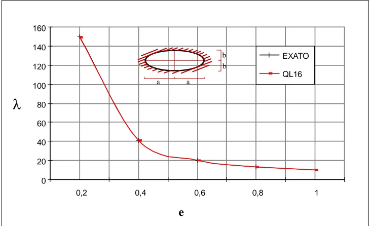
20 % 149. 07 150. 00 0. 620

It is noticeable that the results obtained with the element QL-16 provides excellent outcomes in relation to the “exact” (coincidental curbs). It is also shown that the increase in eccentricity decreases the value of the fundamental frequency, that is, the smaller the eccentricity the larger will the fundamental frequency be (Figure 3).

0 20 40 60 80 100 120 140 160

0,2 0,4 0,6 0,8 1

e

EXATO

QL16 b

a a

b

λ

Figure 3. Frequency parameter variation according to eccentricity.

4 CONCLUSIONS

Numerical simulation of free vibratons of circular and elliptical plates using the Lagrangean quadrilateral element of 16 nodes (QL-16) provides excellent values, when compared to analytical or experimental solutions.

The plate model with finite elements considering the Reissner-Mindlin’s theory allows the use of elements with C0 continuity instead of C1, that are necessary for models that consider kirchhoff’s theory.

The mesh discretization used for element QL-16 converges very fast to the exact solution of the problem. The good performance of this element can by in part explained because it fulfils all essential conditions and criteria for solution convergence.

(10)

ACKNOWLEDGEMENTS

The authors would like to thank CAPES, FIDESA Belém-Pará and CNPq (National Council of Research) for the material (equipment) e financial (scholarships) support offered to the present research programs.

REFERENCES

Timoshenko, S. and Woinowsky-Krieger, S.,( 1970), Teoria de Placas y Laminas, Ediciones Urmo, Spain.

Szilard, R., (1974), Theory and Analysis of Plates - Classical and Numerical Methods, Prentice-Hall, Englewood Cliffs, New Jersey.

Reissner, E., (1945), The effect of transverse shear deformation on the bending of elastic plates, J.Appl.Mech., Vol.12, pp.69-76.

Mindlin, R.D., (1951), Influence of rotatory inertia and shear in flexural motions of isotropic elastic plates, J.Appl.Mech., Vol.18, pp.31-38.

Dawe, D.J. and Roufaeil. O.L., (1980), Rayleigh-Ritz vibration analysis of Mindlin plates, J.Sound Vib., Vol.69, pp.345-359.

Pedroso, L. J., (1983), Maquette Diplodocus - I - Essais d’Interations Fluide Estructures sur le comportment Vibratoires de Plaques en eau. Rapport Interne. EMT/SMTS/VIBR - CEN/SACLAY.

Bathe, K.J. and Dvorkin, E.,( 1985), A four-node plate bending element based on Mindlin/Reissner plate theory and a mixed interpolation, Int.J.num.Meth.Engng., Vol.21, pp.367-383.

Pedroso, L. J., (1986), Qualification Expérimentale des Méthodes de Calculs des Interactions Fluide-Structures en Circuits Tubulaires de Reacteurs Nucleaires. Thése de Doctorat: INSTN/ Laboratoire de Vibrations et Seismes, DEMT/SMTS. Centre d'Etudes Nucléaires de Saclay, France.

Hinton, E. and Huang, H.C., (1986), A family of quadrilateral Mindlin plate elements with substitute shear strain fields, Computers & Strutures, Vol.23, pp.409-431.

Leissa, A.W., (1986), The free vibration of retangular plates," Comp.Meth.Appl.Mech.Engng., Vol. 55, pp.259-300.

Zienkiewicz, O.C. and Taylor, R.L., (1991), The Finite Element Method - Solid and Fluid Mechanics, Dynamics and Non-linearity, McGraw-Will, Vol.2, 4°ed., Singapore.

Oñate, E., (1995), Cálculo de estructuras por el método de elementos finitos - 2°Edición, análisis elástico lineal, Centro Int. Métodos Num. Ingeniería, Barcelona.

Silva, S.F., (1998), Comportamento dinâmico de placas de Reissner-Mindlin utilizando o elemento finito quadrilátero lagrangeano de 16 nós". Thesis of MSc, UnB-FT/EnC,, Brasil.

Nildo Viana, J. et.al., (1998), Análise experimental dinâmica de placas mediamente espessa totalmente livre," Relat. Interno de Ensaio n°30/97, UnB-FT/EnM-LTMD, Brasil.