E
limination-based
C
lassification of
A
dverse
S
patio-
T
emporal
E
xt
r
emes
Zhengzhang Chen1,2, Tatdow Pansombut1,2, William Hendrix3 Doel Gonzalez1,2, Frederick Semazzi1, Alok Choudhary3 Vipin Kumar4, Anatoli V. Melechko1, Nagiza F. Samatova1,2,∗
1North Carolina State University, Raleigh 2
Oak Ridge National Laboratory, Oak Ridge
3North Western University, Evanston 4
University of Minnesota, Minneapolis
∗
Corresponding author: [email protected]
Abstract. Accurate forecasting of extreme events in spatio-temporal systems is a highly underdetermined, yet very important problem. Physics-based models provide unreliable predictions for variables highly related to adverse extreme events, while statistical methods can often only pre-dict linear system responses. In this paper, we proposeForecaster, an algorithm that constructs a forecast-oriented feature elimination-based ensemble of classifiers for robust forecasting of extreme events. In con-trast to existing classification methods that predict the current system state,Forecasterpredicts thefuture phase of the system based on the preceding multivariate data, and it is able to handle underdetermined problems.Forecastersupports nonlinear system behavior as well. Ex-perimental results show thatForecasterincreases prediction accuracy of traditional methods by up to 13% on two seasonal tropical cyclone prediction systems.
Keywords: Forecast-oriented Classification; Feature Elimination-based Ensemble; Extreme Event Prediction; Spatio-temporal Data Mining;
1
Introduction
reduce the severity of the event. For instance, during anticipated low RH sea-sons in Western Africa, authorities must be able to coordinate vaccinations and relief efforts adequately to ensure potential problem areas are targeted, and thus prevent the misdistribution of such efforts.
Fortunately for society, while the adverse effects of extreme events are enor-mous, their occurrences are relatively rare. For example, Hurricane Katrina cost the United States of America over 80 billion dollars and over one thousand lives [17], yet only 92 hurricanes of great destructive magnitude have been reported to strike the United States from 1851-2004, of only 273 hurricanes reported overall during this same period [10].
While the rarity of occurrence of these extreme events is a blessing in the real sense, it is a curse from a statistical machine learning perspective, given the lack of an appropriate number of observational events to build models upon. This issue becomes worse if the characteristics of these events come into con-sideration, as these events can occur in different locations and different times of the year. Furthermore, these events can be influenced by multiple factors which may be nonlinearly correlated, bringing forth the challenges of multivari-ate, spatio-temporal, and inherently nonlinear problems. Thus, considering the
fact of having only a handful of available observational events (m ≈100’s) in
high-dimensional spaces (n≈10,000’s), the existing machine learning methods
easily become hardly suitable for dealing with suchunderdetermined, or
uncon-strained, problems (m << n).
Presently, physics-based models and simulations from first-principles have been making relatively reliable predictions at global spatial scale for ancillary variables, such as climatological factors including Sea Surface Temperature (SST), humidity profiles over land, or wind speed at different heights. However, they provide least reliable predictions for variables that are crucial for impact as-sessment for adverse extreme events including regional precipitation, hurricane intensity and frequency, droughts and floods. In fact, “The sad truth of climate science is that the most crucial information is the least reliable” [19].
As such, statistical methods have emerged to address this need. Unfortu-nately, because our quantitative knowledge about highly non-linear dynamic systems is very meager, modelers often resort to linear regression techniques, such as Least Absolute Deviation (LAD), Least Square Error (LSE), and Pois-son regression, among others, to learn the linear system’s response from various system predictands. For example, hurricane activity is modeled as an LAD re-gression model using observed or simulated system’s parameters, such as SST, Sea Level Pressure (SLP), Vertical Wind Sheer (VWS), and others [9].
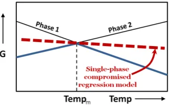
with possibly nonlinear behavior (see, for example, Landau’s theory of phase transitions [15]). Arguably, such a compromised representation (red dashed line in Fig. 1) in a form of a single-phase linear regression model would likely lead to a model with a poor predictive skill for the response variable. For example, hur-ricane activity is the climate system’s response initiated by a liquid-vapor phase transition associated with non-linearly coupled fluctuations in the ocean and the atmosphere. Therefore, linear regression models, while insightful, still offer limited predictability (e.g., 62% prediction accuracy for the observed hurricane activity in North Atlantic region).
Fig. 1.A single-phase “compromised” linear regression model (dashed red line) for a multi-phase physical system that minimizes its Gibbs free energy (solid blue lines) at different phases.
While both regression- and physics-based approaches deserve their own mer-its, in this paper, we draw readers’ attention to a slightly different, yet
comple-mentary,supervised machine learning problem. Namely, given a historic record
about rarely occurring spatio-temporal extreme events of interest, can an algo-rithm learn the complex non-linear relationships between system parameters and the event’s response variable, so that the algorithm can predict what phase the system will likely transition to in some future time and in some spatial region given the knowledge about the system’s parameters defined over global spatial scales before the event’s occurrence?
Slightly more formally, assume that themulti-phase system during the
ex-treme event e = (P, Tf, Le) can be characterized by one of its phases, P ∈
{P1, P2, . . . , Ps} at some future time period Tf and in some event’s spatial
lo-cation region Le. Can the algorithm A predict P given the system’s state(s)
S(T, F, L) described by some spatio-temporal multivariate feature set F over
space L ⊇ Le and time T = (Tf −∆T, Tf)? Note that the temporal
resolu-tion, ∆T, is domain-specific (e.g., 1–5 months for hurricanes). For the sake of
simplicity, we assume that the number s of distinct system’s phases/states is
finite. For example, the hurricane activity can be characterized as being in one
ofP ={above normal, normal, or below normal}phases during hurricane season
Tf ={July-November} in region Le={North America}. We call this problem
To address this problem, we propose an algorithm, calledForecaster, that constructs feature elimination-based ensemble of classifiers for accurate and ro-bust forecasting of adverse spatio-temporal extreme events. Unlike physical
mod-els, which often aim to track event development over afine-grainspatio-temporal
resolution,Forecastersimplifies the problem by utilizing acoarser-grain
spa-tial resolution, and takes an extended time frame into consideration, expanding to a larger scale, such as for seasonal forecasts, with aim to be able to work in lead-time. For example, for a climate-based problem of predicting hurricane activity, we would consider data from the effective hurricane season, spanning from June through November, and work to make such predictions a month(s) in advance.
Furthermore, unlike statistical models that infer linearity and aim to
pre-dict linear responses, Forecaster’s aim is to avoid such inference and treat
the system as behaving nonlinearly. Moreover, unlike models such as the afore-mentioned regression techniques, the intent of our model is not to predict an actual numerical magnitude of the response, instead to seek proper classification into unambiguous groupings, or system’s phases that provide enough informa-tion to make proper decisions, as many statistical models are ultimately being translated into such coarser scales [3] for impact assessment.
Finally,Forecasteris different from traditional classification machine learn-ing methods in a number of ways:
– Forecasterforecasts thefuture phase of the system given its characteris-ticsprior to the time-frame of interest unlike existing classification methods
that predict what state the systemcurrently belongs to, given its current
characteristics.
– Forecasternaturally supports multi-variatespatio-temporal data, which, to the best of our knowledge, no existing classification methodologies are particularly designed for.
– Forecasteris optimized for dealing with highly underdetermined, or un-constrained, classification problems, for which most existing machine learn-ing methods are hardly suitable.
We successfully apply Forecasterto predicting seasonal tropical cyclone
ac-tivity for two regions of interest: North Pacific and North Atlantic. Our
exper-imental results show that Forecaster is able to increase prediction accuracy
of traditional regression-based methods by up to 13% for this problem.
2
Method
We address the aforementioned technical challenges through some key innovative
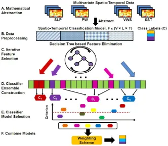
steps underlying theForecaster methodology, summarized with its overview
Fig. 2.Forecaster’s methodology overview.
2.1 Mathematical Abstraction
In traditional supervised classification, a model is learned from a matrix
rep-resentation of the original data with m rows corresponding to a set E of
ob-servations, or events, andn columns corresponding to a set F of features that
characterize each event. In addition, a column vector associates each event with its class from a finite setCof available classes. Once learned, the model predicts
what class the target event defined over the same features F belongs to.
Both the forecasting nature of our problem and the multivariate
spatio-temporal nature of the data necessitate amathematical abstraction that could
transform this data into a mathematical form suitable for a downstream machine learning task, in general, andforecast-driven classification, in particular.
More formally, letV be a set of variables (or factors) that characterize the
system over spatial locationsLand over time periodT. For example, the climate
In the context of the target extreme events, such as hurricanes or droughts, let us also assume that T = T1ST2S. . .STm is divided into m coarse-grain
time intervals during which an extreme event e can occur over some spatial
region Le ⊆ L with some probability. Let us further assume that each time
intervalTj∈T is partitioned into thefine-orcoarse-grain observable Tj,o time
period and the coarse-grain forecastable Tj,f time period (Tj =Tj,oSTj,f and
Tj,o=Ti,o, Tj,f =Ti,f,∀i, j= 1, m).
In the context of hurricane extreme events, for example, each time interval
Tj may correspond to a calendar year that is further divided into a hurricane
seasonTj,f ={July-November}, for which hurricane activity, say inLe={North
Atlantic}region, is being forecasted based on the observed or simulated
month-ly means for climatological factors defined over the entire globe L during the
hurricane pre-season,Tj,o={December-June}.
Furthermore, suppose that each extreme evente can be classified based on
some event-specific classification taxonomy,C. For example, seasonal hurricane
activity, from the impact assessment perspective, could be broadly categorized as “above normal” (say, more than six hurricanes during the hurricane season), “normal,” or “below normal” (say, less than three hurricanes in a season).
Based on the aforementioned notations, the mathematical form can then be
defined as follows (Step A, Fig. 2). Let each row of the matrix correspond to
each time interval Tj, j = 1, m, and let each column of the matrix correspond
to a 3-tuple defined over F = V ×L×T∗,o, where T∗,o is replaced with Tj,o
for the corresponding rowTj. Thus, each (row, col) cell of the matrix if filled in
with the value of the corresponding variable inV for column coldefined at the
corresponding spatial point inLand the corresponding timeTrow,o.
Furthermore, let us assume that a set of known extreme eventsE is defined
over some spatial regionLe, and the class label fromC is assigned to each time
intervalTj based on the accumulative statistics of the observed events overTj,f
time period in regionLe.
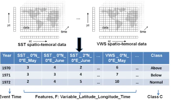
Fig. 3 illustrates this mathematical abstraction using SST and VWS as
vari-ables, or predictands, defined over T = (1970−1972) during the months of
T∗,o={May, June}over (latitude, longitude) spatial grid points for the sea-level
altitude. The class label is inferred based on the historical record of observed
hurricanes in North America duringT∗,f = (July-November) hurricane season.
2.2 Data Preprocessing
Given the aforementioned mathematical abstraction of the original multivariate
spatio-temporal data, the next step of the Forecasteralgorithm is data
pre-processing (StepB, Fig. 2) designed to improve the classifier performance. While the choice of which data preprocessing techniques to employ may be dependent on the type of data under consideration, for preprocessing multivariate,
spatio-temporal data, Forecaster utilizes the following three techniques: temporal
deseasoning,spatial denoising, anddescretization-based denoising.
Fig. 3.A mathematical form for forecast-driven classification of hurricane events.
first transformed into the anomaly time series with zero mean and unit variance per season. This avoids learning a strong seasonality signal and also enables mul-tiple variables with different scales of measurement to be combined into different columns of the same matrix.
Spatial denoising: Since the values of the variable at any location can vary across different time intervalsTjeven at the same observational time periodTj,o,
to lessen the affect of this variability, the anomaly time series at each location point is replaced with its mean anomaly time series taken over the points in the spatial “neighborhood” of this point. This transformation reduces the variance
across differentTj time intervals, thus making the model inference more robust.
Descretization-based denoising: We use a discretization method by Fayyad and Irani [6] to further denoise continuous variables by discretizing their values into categorical intervals based on the entropy minimization heuristics. This technique has been found to be effective in classifying microarray data [21].
2.3 Iterative Decision Tree based Feature Elimination
While the mathematical form proposed in Section 2.1 seems to be suitable for direct use by almost any existing classification technique in machine learning, its highly underdetermined nature prevents this utilization and necessitates
ad-vancements that would enable Forecaster to deal with such unconstrained
problems (i.e., when the size of the feature space|F|=n is significantly larger than the numbermof time intervals,Tj, j= 1, m) .
Forecaster tackles this problem by identifying multiple complementary
sets of discriminatory features from F in order to build a robust ensemble of
classifiers. The proposed methodology relies on the assumption that there are multiple disjoint sets of discriminatory features within the entire feature set, namelyF=F1SF2S. . .SFk, Fi∩Fj=∅. By identifying these discriminatory
Specifically, our methodology employs asupervised, multivariate feature se-lection method thatiteratively selects feature sets until somestopping criterion
is met (StepC, Fig. 2). Under this approach, each iteration produces a subset
of features out of the current feature set, then removes these features from the set so that they cannot be selected again.
We use the CART-decision tree algorithm [2] to select a set of discriminatory features from the available feature space. Basically, CART builds a decision tree by choosing the locally best discriminatory feature at each split step based on the Gini Index Impurity Function [25]. To avoid overfitting, CART employs backward pruning to build smaller, more general decision trees. CART chooses features in a multivariate fashion, which allows the feature selection process to find a set of discriminatory features instead of considering one feature at a time. Forecasteridentifies a candidate set of discriminatory features by building
a decision tree model M using CART, and extracting the features that belong
to the internal nodes ofM (Lines 3–4 in Algorithm 1). In subsequent iterations,
it removes the set of discriminatory features FM corresponding to the model
M from the full feature set F (Line 12) before applying CART-based feature
selection to the rest of the features (those that have not yet been identified as discriminatory features).
Stopping criterion: There are several different criteria that can be used to decide when to stop generating new sets of features (Line 2). Due to high dimen-sionality of our data, we set the threshold on the maximum number of iterations as the stopping criterion.
2.4 Ensemble of Classifiers
Given the set of discriminatory feature sets from Step C above, Forecaster
builds an ensemble of classifiers (StepD, Fig. 2) from the set of selected classifier
models (Step E, Fig. 2) whose predictions are then combined (Step F, Fig. 2)
to make the final prediction.
Building an ensemble of classifiers: For each of the feature sets identified,
we form a new data set DFM by restricting the original data to include only
the selected featuresFM. We then train a separate base classification algorithm
A (e.g., decision tree, SVM, Na¨ıve Bayes, etc.) on the restricted data set to
construct a candidate classifier modelMA. The candidate classifier model MA
will only be included into the ensemble of classifiers if it meets themodel selection criterion(Lines 5–11 in Algorithm 1). The resulting class prediction for the event with the unknown class label is based on the majority voting of the selected
classifiersMA’s. While there are many different voting methods, one can use to
combine predictions made by different classifiers in the ensemble (e.g., [24, 22]), we utilize a simple majority voting, since combining model predictions is outside the focus of the paper.
Algorithm 1: Feature elimination-based ensemble of classifiers
Input:
D: a training dataset over a set of featuresF, and given class labelsC D0: a test dataset over the same features asD, but without class labels A : a basic classification algorithm like decision tree, SVM, andetc.
Output:
C0: predicted class labels for the test setD0
1 InitializeY =∅;
2 whilethe stopping criterion is not met do
3 Run CART-decision tree algorithm onDto get a pruned decision treeM;
4 LetFM be a set of all features that belong to the internal nodes ofM;
5 LetDFM be the restriction ofDto the features inFM;
6 Construct a classifier modelMAby applyingAtoDFM;
7 if MA meets the model selection criterion then
8 LetD0FM be the restriction ofD
0
to the features inFM;
9 ApplyMA toDF0M to produce predicted class labelsC
0
MA;
10 AddCM0 A toY;
11 end
12 Remove features inFM fromF;
13 Remove the data over featureFM fromD;
14 end
15 Predict the class labelsC0 based on a majority vote of the results inY;
16 returnC0;
the base classifier on the particular feature set is below a given threshold. One challenge with this approach is how to select a threshold to distinguish between effective and ineffective classifiers.
In this study, we propose a method for estimating a threshold that reflects a statistically significant improvement over an arbitrary feature selection. To determine this threshold for a given feature set, we randomly sample a large number of feature subsets (e.g., 1000) of the same size and build classifiers for
each of these random feature sets. We then use Student’s t-test to estimate ap
-value for the difference in the training error between the classifier trained on the given feature set and the classifiers trained on the randomly selected feature sets. If this p-value meets a significance criterion (e.g., a significance level of 0.05), then the classifier trained on the given feature set is added to the ensemble.
3
Results
In this section, Forecaster will be tested on two spatio-temporal extreme
3.1 Data
We use the North Atlantic tropical cyclone (TC) count series from 1950 to 2009 from the seasonal (July through November) Atlantic hurricane database (HURDAT) at the National Climatic Data Center to form the class labels. This dataset includes the hurricanes, tropical storms, and tropical depressions that occurred in the entire Atlantic basin. We also utilize the North Pacific seasonal (June through October) TC count series from 1970 to 2006 provided by the Central Weather Bureau [3]. These series cover tropical storms and typhoons in
the area between 21–26◦N and 119–125◦E.
According to Chu et al. [3], the observed TC count series of North Pacific
region were classified into three classes: “below,” “normal,” and “above,” with a distribution of 40% as “normal” and 30% each as “below” and “above.” (Years with fewer than three TCs are classified as “below,” and years with at least five TCs are classified as “above.”) In the case of the North Atlantic region, years with TC counts fewer than five are classified as “below,” and TC counts larger than seven are classified as “above.”
We use monthly mean sea level pressure (SLP), precipitable water (PW), sea surface temperature (SST), and tropospheric vertical wind shear (VWS) data in order to predict the North Atlantic and North Pacific TC class. SLP and
PW are NCEP/NCAR reanalysis datasets. They are available at a 2.5◦×2.5◦
latitude and longitude resolution. SST is from the NOAA Climate Diagnostic
Center in Boulder, Colorado, at a resolution of 2◦×2◦ latitude and longitude.
VWS is calculated by computing the square root of the sum of the square of the difference in zonal wind component between 850 and 200 hPa levels and the square of the difference in meridional wind component between 850 and 200 hPa levels [4] from NCEP/NCAR reanalysis data.
The global SLP, PW, VWS, and SST datasets in preceding June are used for the North Atlantic TC class prediction. The four variables combined contribute
47,556 features toF as columns in the matrix form as described in Section 2.1.
For comparative purposes, only the data for the same type of four variables in
preceding May over the western North Pacific (0–30◦N and 100–180◦E) region
with 1,652 features is used for the North Pacific TC class prediction.
3.2 Performance Evaluation Method
Because of the small sample size of the spatio-temporal data, leave-one-out cross
validation (LOOCV) is employed to evaluate Forecaster’s robustness. We
utilize several metrics to evaluateForecaster’s performances: accuracy, Heidke
Skill Score (HSS) [11], Peirce Skill Score (PSS) [16, 11], and Gerrity Skill Score (GSS) [12]. Accuracy is defined as the ratio of the number of correctly classified data points to the total number of data points in the test set.
3.3 Forecaster Performance Comparison
Table 1 compares Forecaster’s performance to seasonal tropical cyclone
: SST : SLP : PW +: VWS
PDO
Nino 3 MDR
ESPI
(a) Model 1
: SST : SLP : PW +: VWS
AO
NAO
ENSO
(b) Model 2
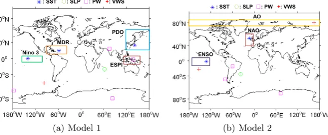
Fig. 4.Features selected by two models for North Atlantic tropical cyclone prediction
North Pacific region, there is a roughly 8% increase over the 65.5% reported
by Kim et al. [14]. For the North Atlantic Region, Forecaster achieves an
increase of nearly 13% in accuracy and GSS and nearly 20% in HSS and PSS.
Table 1.LOOCV performance for seasonal TC class prediction
Metric North Pacific North Atlantic
ForecasterChu [3] Kim [14] ForecasterWebster [13]
Accuracy 0.73 0.623 0.655 0.75 0.621
HSS 0.584 0.424 0.483 0.60 0.437
PSS 0.596 0.424 0.521 0.62 0.446
GSS 0.603 0.541 0.592 0.63 0.567
3.4 Climatological Relevance
Fig. 4 shows two discriminating feature subsets included into the two selected classifier models. In the case of Model 1 (Fig. 4(a)), among all three SST features
(star-shaped in Fig. 4(a)), one is located in the Ni˜no 3 region. Ni˜no 3 SST
has a strong correlation with Atlantic hurricane activity [8, 13]. Another SST feature belongs to the hurricane main development region (MDR). SST values in MDR have been shown to contribute to the hurricanes generated in the MDR region [18, 26]. The last SST feature is from Pacific Decadal Oscillation (PDO) region. Shifts in the PDO phase can have significant implications for Atlantic hurricane activity, and significant differences are shown in hurricane intensity
between El Ni˜no and La Ni˜no years when the PDO is in warm phase [23].
North Atlantic tropical cyclones [20]. Our models also find some unknown pat-terns like PW in ESPI region and VWS in AO regions, which might affect the North Atlantic tropical cyclone activities as well.
4
acknowledgements
This work was supported in part by the U.S. Department of Energy, Office of Science, the Office of Advanced Scientific Computing Research (ASCR) and the Office of Biological and Environmental Research (BER) and the U.S. National Science Foundation (Expeditions in Computing). Oak Ridge National Labora-tory is managed by UT-Battelle for the LLC U.S. D.O.E. under contract no. DEAC05-00OR22725.
5
Conclusion
In this paper, the spatio-temporal extreme event prediction problem has been
modeled as a supervised machine learning problem. We have presented
Fore-caster, a feature elimination-based ensemble of classifiers for spatio-temporal
extreme events prediction algorithm.Forecaster can iteratively select
smal-l subsets of discriminating features in a musmal-ltivariate and non-smal-linear fashion.
This property letsForecastereffectively and efficiently deal with the
forecast-oriented classification of spatio-temporal extreme events problem as well as oth-er highly undetoth-ermined classification problems. Our expoth-erimental results have
shown thatForecastercan improve prediction accuracy by up to 13% on two
seasonal tropocial cyclone datasets.
References
1. S.J. Connor A.P. Morse A.M. Molesworth, L.E. Cuevas and M.C. Thomson. En-vironmental risk and meningitis epidemics in Africa. EID, 9(10):1287–1293, 2003. 2. L. Breiman, J. Friedman, R. Olshen, and C. Stone. Classification and regression
trees. Wadsworth and Brooks, Monterey, CA, 1984.
3. P.S. Chu, X. Zhao, C.T. Lee, and M.M. Lu. Climate prediction of tropical cyclone activity in the vicinity of Taiwan using the multivariate least absolute deviation regression method. Terr. Atmos. Ocean. Sci., 18(4):805–825, October 2007. 4. J. D. Clark and P. S. Chu. Interannual variation of tropical cyclone activity over
the Central North Pacific. JMSJ, 80(3):403–418, 2002. 5. J.B. Elsner. Tracking hurricanes. AMS, 84:353–356, 2001.
6. U. M. Fayyad and K.B. Irani. Multi-interval discretization of continuous-valued attributes for classification learning. InIJCAI, pages 1022–1027, 1993.
7. J.W. Gibbs. On the equilibrium of heterogeneous substances. Transactions of the Connecticut Academy of Arts and Sciences, 3:108–248, 343–534, 1874-1878. 8. S.B. Goldenberg and L.J. Shapiro. Physical mechanisms for the association of El
9. W.M. Gray, C.W. Landsea, P.W. Mielke, Jr., and K. J. Berry. Predicting Atlantic seasonal hurricane activity 6-11 months in advance. Weather Forecast., 7:440–455, September 1992.
10. E.S. Blake E.N. Rappaport J.D. Jarrell, C.W. Landsea. The deadliest, costliest, and most intense united states hurricanes of this century (and other frequently requested hurricane facts). NOAA Technical Memorandum NWS TPC-4, 2005. 11. I. T. Jolliffe and D. B. Stephenson. Forecast Verification: A Practitioner’s Guide
in Atmospheric Science. Wiley and Sons, 2003.
12. P. Joseph and Jr. Gerrity. A note on Gandin and Murphy’s equitable skill score.
Monthly Weather Review, (120):2709–2712, 1992.
13. H. M. Kim and P. J. Webster. Extended-range seasonal hurricane forecasts for the North Atlantic with a hybrid dynamical-statistical model. Geophys. Res. Lett., 37(21):L21705, 2010.
14. H. S. Kim, C. H. Ho, P. S. Chu, and J. H. Kim. Seasonal prediction of summertime tropical cyclone activity over the East China Sea using the least absolute deviation regression and the Poisson regression. Int. J. Climato., 30(2):210–219, 2010. 15. L. Landau. The theory of phase transitions. Nature, 138(3498):840–841, 1936. 16. C. S. Peirce. The numerical measure of the success of predictions.Science, (4):453–
454, 1884.
17. C.W. Landsea D. Collins M.A. Saunders R.A. Pielke Jr., J. Gratz and R. Musulin. Normalized hurricane damage in the United States: 1900-2005.Nat. Hazards Rev., 9(1):29–42, 2008.
18. M.A. Saunders and A.R. Harris. Statistical evidence links exceptional 1995 Atlantic hurricane season to record sea warming. JGRL, 24:1255–1258, 1997.
19. Q. Schiermeier. The real holes in climate science. Nature, 463:284–287, 2010. 20. J.P. Kossin S.J. Camargo and M. Sitkowski. Climate modulation of North Atlantic
hurricane tracks. Journal of Climate, 23:3057–3076, 2010.
21. A.C. Tan and D. Gilbert. Ensemble machine learning on gene expression data for cancer classification. Applied bioinformatics, 2(3 Suppl), 2003.
22. D. Tao, X. Tang, and et.al. Asymmetric bagging and random subspace for support vector machines-based relevance feedback in image retrieval. IEEE T. Pattern Anal., 28(7):1088–1099, July 2006.
23. C.J. Melick A.R. Lupo T.K. Latham T.H. Magill, J.V. Christopher and P.S. Mar-ket. The interannual variability of hurricane activity in the art. National Weather Digest, 32:1–15, 2008.
24. A. Tsymbal, S. Puuronen, and D.W. Patterson. Ensemble feature selection with the simple Bayesian classification. Information Fusion, 4(2):87–100, 2003. 25. I. H. Witten and E. Frank. Data mining: practical machine learning tools and
techniques with Java implementations.ACM SIGMOD Record, 31(1):76–77, 2002. 26. L. Xie, T. Yan, and L. Pietrafesa. The effect of Atlantic sea surface temperature dipole mode on hurricanes: Implications for the 2004 Atlantic hurricane season.