Dynamic backtracking for general CSPs.

University of Windsor University of Windsor

Scholarship at UWindsor

Scholarship at UWindsor

Electronic Theses and Dissertations Theses, Dissertations, and Major Papers

1-1-2007

Dynamic backtracking for general CSPs.

Dynamic backtracking for general CSPs.

Kan Yu

University of Windsor

Follow this and additional works at: https://scholar.uwindsor.ca/etd

Recommended Citation Recommended Citation

Yu, Kan, "Dynamic backtracking for general CSPs." (2007). Electronic Theses and Dissertations. 7035.

https://scholar.uwindsor.ca/etd/7035

Dynamic Backtracking for General CSPs

by

Kan Yu

A Thesis

submitted to the Faculty o f Graduate Studies through the School o f Computer Science in Partial Fulfillment o f the Requirements for

the Degree o f Master o f Science at the University o f Windsor

Windsor, Ontario, Canada 2007

Library and Archives Canada

Bibliotheque et Archives Canada

Published Heritage Branch

395 Wellington Street Ottawa ON K1A 0N4 Canada

Your file Votre reference ISBN: 978-0-494-35062-1 Our file Notre reference ISBN: 978-0-494-35062-1 Direction du

Patrimoine de I'edition

395, rue Wellington Ottawa ON K1A 0N4 Canada

NOTICE:

The author has granted a non­

exclusive license allowing Library

and Archives Canada to reproduce,

publish, archive, preserve, conserve,

communicate to the public by

telecommunication or on the Internet,

loan, distribute and sell theses

worldwide, for commercial or non­

commercial purposes, in microform,

paper, electronic and/or any other

formats.

AVIS:

L'auteur a accorde une licence non exclusive

permettant a la Bibliotheque et Archives

Canada de reproduire, publier, archiver,

sauvegarder, conserver, transmettre au public

par telecommunication ou par I'lnternet, preter,

distribuer et vendre des theses partout dans

le monde, a des fins commerciales ou autres,

sur support microforme, papier, electronique

et/ou autres formats.

The author retains copyright

ownership and moral rights in

this thesis. Neither the thesis

nor substantial extracts from it

may be printed or otherwise

reproduced without the author's

permission.

L'auteur conserve la propriete du droit d'auteur

et des droits moraux qui protege cette these.

Ni la these ni des extraits substantiels de

celle-ci ne doivent etre imprimes ou autrement

reproduits sans son autorisation.

In compliance with the Canadian

Privacy Act some supporting

forms may have been removed

from this thesis.

While these forms may be included

in the document page count,

their removal does not represent

Conformement a la loi canadienne

sur la protection de la vie privee,

quelques formulaires secondaires

ont ete enleves de cette these.

Abstract

There are two categories o f CSPs: binary CSPs and general CSPs. A binary CSP has only unary and binary constraints. A unary constraint restricts the value of one variable while a binary constraint restricts the values of two variables. A general CSP may have constraints that restrict more than two variables. Many algorithms have been developed to solve CSPs. Dynamic Backtracking and Constraint-directed Backtracking algorithms (CDBT) are two o f them. This thesis introduces a new general CSP-solving algorithm - Constraint-directed Dynamic Backtracking (CDDBT) that combines the advantages o f Dynamic Backtracking and CDBT.

Dedication

To

Acknowledgements

I would like to thank my supervisor Dr. Scott Goodwin, for his guidance, for his academic advice, and for his support. I am also grateful for the scholarships provided by the University o f Windsor.

I also extend my appreciation to the members of my committee - Dr. Dan Wu and Dr. Myron Hlynka, for their feedback and academic advice. I would like to thank Dr. Richard Frost, the chair o f my committee, for his guidance and academic advice when I wrote my 510 survey.

I would like to thank Dr. Liwu Li, for his guidance. His sudden and unexpected death was a shock to everyone. He is sincerely missed.

I would like to thank Robert George Price, for his academic advice and help. I would also like to thank Robert Effinger, for his comments on Dynamic Backtracking.

I want to especially thank my parents for their love and full support.

Table of Contents

Abstract... iii

Dedication... iv

Acknowledgements... v

List o f Tables...viii

List o f Figures... ix

1 Introduction...1

1.1 Definition o f CSP... 1

1.2 Examples o f CSP...2

1.3 Motivation...3

2 Background...5

2.1 Basic Concepts... 5

2.1.1 Unary, Binary and General Constraints...5

2.1.2 Density and Tightness... 5

2.1.3 Constraint Graphs... 6

2.1.4 Satisfiability and Consistency... 7

2.1.5 Search Ordering... 7

2.2 CSP-solving Techniques... 9

2.2.1 General Discussion...9

2.2.2 Backtracking...10

2.2.3 AC-3 algorithm... 10

2.2.4 Systematic and Non-systematic Search... 12

2.2.5 Performance o f CSP Algorithms... 14

2.3 Dynamic Backtracking... 15

2.3.1 Problem Addressed... 15

2.3.2 Definitions... 15

2.3.3 The Algorithm...16

2.3.4 Example... 17

2.3.5 Related Work... 23

2.4 General C SPs... 25

2.4.1 Introduction...25

2.4.2 Early Research... 25

2.4.3 Later Research... 26

2.4.4 Current Research... 27

2.4.5 CDBT...28

3 CDDBT... 32

3.1 Methodology...32

3.2 The Algorithm... 33

3.3 Proof...38

4.1 Random General CSP Generator... 41

4.1.1 Methodology... ... 41

4.1.2 A random CSP example...43

4.2 Experiment Data...46

4.2.1 Target Property: number o f variables... 47

4.2.2 Target Property: domain size... 49

4.2.3 Target Property: number o f constraints... 51

4.2.4 Target Property: arity... 53

4.2.5 Target Property: tightness o f constraint... 54

5 Results and Analysis... 57

6 Conclusion and Future Work... 67

Appendix: testing environment... 69

References...70

Vita Auctoris... 76

List of Tables

Table 3-1 Notation o f CDDBT...34

Table 4-1 Three criteria for comparing the performance o f CDDBT and CDBT... 46

Table 4-2 Experiment #l(number o f variables vs. CPU runtime)... 47

Table 4-3 Experiment #1 (number o f variables vs. node checks)... 48

Table 4-4 Experiment #1 (number o f variables vs. consistency checks)... 48

Table 4-5 Experiment #2(domain size vs. CPU runtime)... 49

Table 4-6 Experiment #2(domain size vs. node checks)...50

Table 4-7 Experiment #2(domain size vs. consistency checks)...51

Table 4-8 Experiment #3(number o f constraints vs. CPU runtime)... 51

Table 4-9 Experiment #3 (number o f constraints vs. node checks)... 52

Table 4-10 Experiment #3(number o f constraints vs. consistency checks)... 53

Table 4-11 Experiment #4(arity vs. CPU runtime)... 53

Table 4-12 Experiment #4(arity vs. node checks)...54

Table 4-13 Experiment #4(arity vs. consistency checks)...54

Table 4-14 Experiment #5(tightness o f constraint vs. CPU runtime)... 55

Table 4-15 Experiment #5(tightness o f constraint vs. node checks)... 56

Table 4-16 Experiment #5(tightness o f constraint vs. consistency checks)... 56

List of Figures

Figure 1-1 8-queens problem... 3

Figure 2-1 Aconstraint graph (Russell & Norvig, 2003)...6

Figure 2-2 Backtracking search (Russell & Norvig, 2003)...10

Figure 2-3 AC-3 (Russell & Norvig, 2 0 0 3 )...11

Figure 2-4 Dynamic Backtracking (Ginsberg, 1993)... 16

Figure 5-1 Experiment #l(number o f variables vs. CPU runtime)... 58

Figure 5-2 Experiment #l(number o f variables vs. consistency checks)...59

Figure 5-3 Experiment #2(domain size vs. CPU runtime)... 60

Figure 5-4 Experiment #2(domain size vs. consistency checks)... 60

Figure 5-5 Experiment #3 (number o f constraints vs. CPU runtime)...61

Figure 5-6 Experiment #3 (number o f constraints vs. consistency checks)... 62

Figure 5-7 Experiment #4(arity vs. CPU runtime)... 62

Figure 5-8 Experiment #4(arity vs. consistency checks)... 63

Figure 5-9 Experiment #5 (tightness o f constraint vs. CPU runtime)... 64

Figure 5-10 Experiment #5(tightness o f constraint vs. consistency checks) ...64

1 Introduction

In Artificial Intelligence (AI), a lot of problems can be represented as Constraint Satisfaction Problems (CSPs). We can find them in many fields of AI such as machine vision, belief maintenance, scheduling problems, temporal reasoning, graph-coloring problems, bioinformatics, and so on.

1.1 Definition of CSP

One definition o f CSP from (Russell & Norvig, 2003) is:

“A constraint satisfaction problem (or CSP) is defined by a set o f variables, Xi, X2, . . . , Xn, and a set o f constraints, Ci, C2, . . . , Cm. Each variable X* has a nonempty domain D, o f possible values.”

Another definition from (Tsang, 1993) is:

“A constraint satisfaction problem is a triple: (Z, D, C) where Z = a finite set of variables { Xi, X2, . . . , Xn }.

D = a function which maps every variable in Z to a set o f objects o f arbitrary type.

C = a finite (possibly empty) set of constraints on an arbitrary subset of variables in Z.”

There are two categories o f CSPs: binary CSPs and general CSPs. A binary CSP has only unary and binary constraints. A unary constraint restricts the value of one variable while a binary constraint restricts the values o f two variables. A general CSP may have constraints that restrict more than two variables. Many algorithms have been developed to solve CSPs. Dynamic Backtracking (Ginsberg, 1993) and Constraint-directed Backtracking algorithms (CDBT) (Pang, 1998) are two of them.

1.2 Examples of CSP

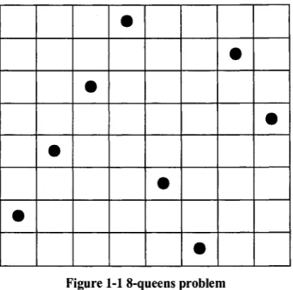
There are many CSPs in different areas. For example, one well-known CSP is the 8-queens problem. A chess player named Max Bezzel originally proposed this problem in 1848. Over the years, many mathematicians and Computer Scientists have worked on the problem. The problem is to put eight queens on an 8x8 chessboard such that no two queens can attack each other. The 8-queens problem has 92 distinct solutions ( 1 2 solutions if not counting symmetry operations).

Figure 1-1 8-queens problem

Another well-known but harder CSP problem is the car sequencing problem. The goal of the problem is to find an optimal arrangement o f cars along a production line, given production requirements, option requirements and capacity constraints. The detailed description can be found in (Tsang, 1993). Other famous examples are Crossword Puzzles, Map-Coloring problems, and so on.

1.3 Motivation

1. Dynamic Backtracking for binary constraints continues to be a focus of research (Effmger & Williams, 2006) and (Zivan, Shapen, Zazone, & Meisels, 2006). Its concept of "eliminating explanation" can be applied to both binary and non-binary CSPs. However, Dynamic Backtracking with non-binary cases has not been completely investigated.

Dynamic Backtracking in the binary case can be carried over to the non-binary case.

2 Background

2.1 Basic Concepts

2.1.1 Unary, Binary and General Constraints

There are two categories o f CSPs: binary CSPs and general CSPs. General CSPs are also called non-binary CSPs. A binary CSP has only unary and binary constraints. A unary constraint restricts the value of one variable while a binary constraint restricts the values of two variables. A general CSP may have constraints that restrict more than two variables. In (Rossi, Petrie, & Dhar, 1990), the authors claim that it is possible to convert any non-binary CSP to a binary CSP having the same solutions. However, the efficiency of converting and then applying a binary CSP-solving algorithm may not be as good as simply applying a non-binary CSP-solving algorithm directly.

2.1.2 Density and Tightness

_ . the _ number _ o f _constraints

D e n sity =

---the _ number _ o f _ all _ possible _ constraints

For example, if a CSP has three variables {Vi, V2, V3}, we have seven all possible constraints, which are {Vi}, {V2}, {V3}, {Vh V2}, {Vi, V3}, {V2, V3}, and (Vi, V2, V3}. The number o f all possible constraints is defined \)y 2 ,he- number- of-™ ,abks- 1 . If the CSP has only one constraint Ci= (V), V2}, the density o f the CSP is = 0.14.

, .. . the_number o f_ v a lid tuples_of a constraint I ightness_ oj _ a _ constrain £=----

---the_number_ o f _ all_ possible_ tuples_ o f _ a _ constraint

2, 3, 4}, all possible tuples o f Ci are (1, 1), (1, 2), (1, 3), (2, 1), (2, 2), and (2, 3). The number o f all possible tuples of Ci is defined b y |D ,|x |D 2| = 2 x 3 = 6 . If the CSP has

3 three valid tuples (2, 1), (2, 2), and (2, 3), the tightness of Ci is— = 0.5.

6

Some researchers use an opposite definition:

the_num ber_of _invalid_tuples_of _ a _constraint Tightness_oj _ a _constraint=---

—---the_num ber_of _all_possible_tuples_of _a_constraint

2.1.3 Constraint Graphs

A binary CSP can be represented as an undirected graph. In the graph, the nodes stand for variables and the edges stand for binary constraints. A General CSP can be represented as a hypergraph. Graph theory has a significant influence on CSP research. A CSP can be unconnected (Figure 2.1).

N T

Queensland

\

W estern Australia South Australia _New South W iles

i

/

(a)

0

viewed as a constraint satisfaction problem. Tire goal is to assign colors to each region so that no neighboring regions have the same color, (b) The map-coloring problem represented as a constraint graph.

Figure 2 -1 A constraint graph (Russell & Norvig, 2003)

2.1.4 Satisfiability and Consistency

Two fundamental concepts in CSP are satisfiability and consistency. In (Tsang, 1993), the author introduces the concept of compound label. A compound label is an assignment o f values to variables like (<Variablel, value 1>, <Variable2, value2>,. . . , cVariableX, ValueX>). A constraint can also be viewed as a set of legal compound labels. He also introduces a simple definition o f satisfiability, which is “a compound label X satisfies a constraint C if and only if X is an element o f C”. Based on this simple definition of satisfiability, related concepts are built such as satisfiable, k-satisfies, and k-satisfiable (Tsang, 1993).

Consistency is another essential concept in CSP. According to (Tsang, 1993), “a CSP is 1-consistent if and only if every value in every domain satisfies the unary constraints on the subject variable. A CSP is k-consistent, for k greater than 1, if and only if all ( k -1) compound labels which satisfy all relevant constraints can be extended to include any additional variable to form a k-compound label that satisfies all the relevant constraints”.

Satisfiability and consistency have a close relationship. They support many other important concepts and theorems in CSP research, for example, the concepts of node consistency (NC, same as 1-consistency), arc consistency (AC, same as 2-consistency), and path consistency (PC, same as 3-consistency in binary CSP).

2.1.5 Search Ordering

authors introduce three heuristics: the minimum remaining values (MRV) heuristic, the degree heuristic, and the least-constraining-value heuristic. The MRV heuristic picks a variable that has fewer remaining values. The degree heuristic picks a variable that is “involved in the largest number o f constraints on other unassigned variables”. The least-constraining-value heuristic picks a value that “rules out the fewest choices for the neighboring variables in the constraint graph.”

For example, we have a CSP, which has ten variables {Vi, V2, . . V10}. Each variable has the same domain {1, 2, ..., 100}. After we assign 1 to V], we are going to pick the next variable. V2 to V9 have more than one remaining value. V10 has one only value left, which is 5. Instead o f picking V2, the MRV heuristic will pick V10. If it cannot assign 5 to V10, we need backtrack. It may save time since we don’t need to assign values to variables between V2 and V9.

2.2 CSP-solving Techniques

2.2.1 General Discussion

Modeling or representing a problem as a CSP is one area in CSP research. Plow to solve a CSP is another important area. Over thirty years, CSP researchers have developed different kinds o f methods or algorithms that can solve CSPs.

(Tsang, 1993) classifies techniques in CSP-solving into three categories: problem reduction, search, and solution synthesis. Each category corresponds to one chapter in his book. In the problem-reduction chapter, the author mainly talks about NC, AC, and PC algorithms. In (Russell & Norvig, 2003) problem-reduction methods are classified as constraint propagation methods. In the search chapter, Tsang introduces three categories o f search strategies: general search strategies, lookahead strategies, and gather-information-while-searching strategies. Most o f the CSP-solving algorithms can be found in this chapter such as Backtracking, Forward Checking, Backjumping, Backchecking, Backmarking, and so on. In the solution-synthesis chapter, the author mainly talks about GENET. In the rest of the chapters, the author introduces other important techniques like stochastic search.

2.2.2 Backtracking

The Backtracking algorithm is a fundamental CSP-solving algorithm, which is the basis o f many other algorithms. It was first formally introduced by (Bitner & Reingold, 1975). However, the basic idea of Backtracking can be traced back to the 19th century. Furthermore, it is often compared with other algorithms to evaluate their performance. Backtracking, or backtracking search, is a depth-first search. It is shown in Figure 2.2.

function BACKTRACKING-SEARCH(esp) returns a solution, o r failure retu rn RECURSIVE-BACKTRACKING({ }, csp)

function RECTRSIVE-BACKTRACKING(cisA%rmi«?i, csp) returns a solution, or failure

i f assignment is co m p lete then return a s s ig n m e n t

v a r « - SELECT-UNA5SIGNED-VARIABLE(VARIABLES[csp], a s s i g m i e n t . c s p)

f o r e a c h v a lu e in QRDER-DOMAIN-VALUESf iw r, a s s ig n m e n t, c sp) do

if va lu e is c o n siste n t with iu>*itirimenta c c o rd in g to CONSTRAINTS[c#p] then add { ik it = v a lu e } to m erit

r e s u lt RECURSIVE-BACKTRACKING( assignment, c s p)

if ‘re su lt ^ f a i h m then return i<

rem o v e { v a r = >'oJne) fro m a ssn p in a »f

retu rn fa ilu r e

Figure 2-2 Backtracking search (Russell & Norvig, 2003)

Backtracking tries to assign a value to a variable. If it does not violate any constraints, it will assign a value to the next variable. If it fails to assign a value, it will backtrack to the previous variable.

2.2.3 AC-3 algorithm

One important class of CSP-solving algorithms is called “arc consistency” algorithms (Mackworth, 1977a). Achieving consistency is also called problem reduction (Tsang, 1993), problem relaxation, or constraint propagation. In (Montanari, 1974), the author introduces the concept o f constraint networks and propagation using path consistency. This approach was popularized by (Waltz, 1975). By achieving certain consistency (NC, AC, or PC), the problem is reduced by eliminating redundant information from

domains and constraints. In other words, “an arc consistency algorithm can be thought of as a simplification algorithm which transforms the original problem into a simpler version that has the same solutions” (Nadel, 1989). Consistency concepts are so defined to guarantee it. Another property o f arc consistency mentioned in (E. C. Freuder, 1982) is that in any binary CSP, if its constraint graph can be represented as a tree, a backtrack-free search can be obtained if node and arc consistency are obtained.

NC, AC, and PC are different levels of consistency. In (Nadel, 1989), the author classifies AC algorithms into two categories: partial arc consistency algorithms

( A C ^ , A C ^, AC ^3, and A C 3'3 ) and full arc consistency algorithms (AC1, AC2, and AC3). In (Tsang, 1993), the author lists another AC algorithm: AC4. AC-3 (Mackworth, 1977a) is a widely-used algorithm:

function AC-3( csp)m u n is the CSP, possibly with reduced domains inputs: cap, a binary CSP with variables {A'j, A<s, .... A* } local variables: queue,a queue o f arcs, initially all the arcs in csp is M r lim te is not empty do

A', Y j) — REMOVE-FIRS T (q u eu e)

if RE'fOVE-lNCONSISTENT-VALU1S(A',, A j ) then for each .¥ * in NEIGHBORS!A',]

add (A*. Xi) to queue

function REMOVE- INCONSISTENT-VALUES( A ',, A'*) returns true if f w e remove a value

tv moved — fa k e

for each, x in DOMAIN[.V>] do

if no value yin DGMAIX[A\] allows (x,y)to satisfy the constraint between A ; and X j

d m delete xfrom DOMAIN[XjJ; removed— true

return removed

Figure 2-3 AC-3 (Russell & Norvig, 2003)

2.2.4 Systematic and Non-systematic Search

Systematic search (global search) and non-systematic search (local search) are two categories of CSP-solving methods. In (F. Freuder, Dechter, Ginsberg, Selman, & Tsang, 1995), Dechter credits the work done in (Pearl, 1984): “Systematic algorithms have two properties (1) Do not leave any stone unturned (completeness), and (2) do not turn any stone more than once (efficiency).” Dechter claims that greedy non-systematic algorithms may “leave many stones unturned and may also turn the same stone multiple times”. Here, efficiency does not mean performance. She also claims that systematic search can beat non-systematic search sometimes, and vice versa. The following papers discuss systematic search and/or non-systematic search. Others can be found in later Sections.

In (Minton, Johnston, Philips, & Laird, 1990), the problem addressed by the authors is meaningful progress on how to solve large-scale constraint satisfaction and scheduling problems. Three previous papers referred to by the authors are (Stone & Stone, 1987), (Johnston & Adorf, 1989), and (Adorf & Johnston, 1990). The authors develop a new heuristic called the min-conflicts heuristic that captures the idea of Guarded Discrete Stochastic (GDS) Network. The main idea o f the min-conflicts heuristic is to minimize the number of conflicts by assigning a new value to the variable, which is in conflict. The authors do experiments by employing three search strategies (hill-climbing, informed backtracking, and best-first search) with the min-conflicts heuristic. They claim that min-conflicts hill-climbing and min-conflicts backtracking perform much better than basic backtracking on the n-queens problem. They also claim that the min-conflicts heuristic is less effective on problems like coloring sparsely-connected graphs. They state that these problems have a few highly-critical constraints and many less important constraints. This paper has been cited by many researchers such as (Minton, Johnston, Philips, & Laird, 1992) and (Ginsberg, 1993).

After two years, four authors presented another paper (Minton et al., 1992). They analyzed the min-conflicts heuristic. They state that (Johnston & Adorf, 1989) and (Adorf & Johnston, 1990) inspired their heuristic. Adorf and Johnston developed a neural network called GDS network. Minton et al. raise a question “why does the GDS network perform so well”. They state both a non-systematic search hypothesis and an informedness hypothesis. They claim that the informedness hypothesis is the reason. By capturing the idea o f GDS, the authors state the min-conflicts heuristic. The heuristic assigns a value o f a variable in conflict while the value minimizes the number of conflicts. The authors also claim that many search strategies can use the method of repairing an inconsistent assignment except the hill-climbing strategy. This paper has been cited by many researchers such as (Davenport, Tsang, Zhu, & Wang,

1994) and (F. Freuder et al., 1995).

2.2.5 Performance of CSP Algorithms

In (Nadel, 1988), the author evaluates some CSP-solving algorithms on n-queens and confused n-queens problems. He claims that Forward Checking (FC) performs best among these algorithms. In (Kumar, 1992), the author lists three schemes of CSP-solving techniques: backtracking, constraint propagation, and constraint propagation inside backtracking. The author claims that the drawbacks for backtracking are thrashing (Gaschnig, 1979) and redundant work. For example, algorithms using a backtracking mechanism may keep backtracking for the same reason. Kumar (1992) claims that there are two possible reasons for thrashing: node inconsistency and arc inconsistency (Mackworth, 1977a). On the other hand, he also states that constraint propagation is more expensive than simple backtracking in most cases. So the author raises a question - “how much constraint propagation is useful.” In (Mackworth & Freuder, 1993), the authors compare and analyze the complexity of many finite CSP (FCSP) algorithms such as AC-1, AC-2, AC-3, and AC-4. They state that it is important to identify tractable problem classes that are specific classes with tractable solution techniques.

2.3 Dynamic Backtracking

2.3.1 Problem Addressed

In (Ginsberg, 1993), the problem addressed by the author is that meaningful progress is sometimes removed in existing backtracking methods. For example, Backtracking suffers from thrashing. Two previous papers referred to by the author are Dependency-directed backtracking (Stallman & Sussman, 1977) and Backjumping (Gaschnig, 1979). They both suffer from this problem. In (Ginsberg, 1993), the author introduces a new algorithm called Dynamic Backtracking that can solve this problem.

2.3.2 Definitions

Ginsberg uses another definition o f the CSP. He defines a CSP as “a set I o f variables; for each i G /, there is a set of Vt o f possible values for the variable i. k is a set of constraints, each a pair (J, P) where J= ( / '/ , .. . ,jk) is an ordered subset of /a n d P is a subset of Vn x • • • x Vjk Because i is unique, the author uses it to indicate both a

variable and the index of a domain.

The most important concept the author introduced is the concept of an eliminating explanation. “Given a partial solution P l to a CSP, an eliminating explanation for a

variable i is a pair (v, S) where v G V f and 5 c P.” P is the corresponding set of variables for P. The underlying meaning of eliminating explanation is that i cannot be set to v because of the values that are already set by P to the variables in S. An eliminating mechanism e is a function. It takes two inputs: a partial solution P and a

2.3.3 The Algorithm

The author reconstructs the depth-first search algorithm and the Backjumping algorithm with his notations of CSP and the concept o f eliminating explanation. Then he gives the algorithm o f Dynamic Backtracking:

A l g o r i t h m 4 .3 ( D y n a m ic backtracking) Given m inputs a constrainl-satisfaction prob­ lem and an elim ination mechanism e:

1. Set P -i“ E i =! 0 for each i€ I .

I, I f I I return P . Otherwise, select a variable i € I — P . Set E i = JS» U e(F, f).

S. Set S ~ Vi - E i. I f S is nonem pty, choose an d e m e n t v £ S . Add ( t , «) to P and return to step S.

I I f S is em pty, we m u st ham E, i;.- let E be the set o f all variables appearing in the

explanations fo r each elim inated value.

5. I f E 0 , return failure. Otherwise, let (j, vj) be the last entry in P that binds a variable appearing in E . Remove ( j,ty} fro m P and, fo r each variable k assigned a value after j , remove from. Eu any eliminating explanation that involves j . Add ( v j , E P P ) to Ej and return to step $.

Figure 2-4 Dynamic Backtracking (Ginsberg, 1993)

2.3.4 Example

Given a simple CSP: Variables: V ,,V2,V3

Domains: Di=D2=D3= {1, 2} Constraints: V i^ V2, V2^ V3, V3^ Vi

Initially:

Eliminating Explanations Assigned Value

Vi V2 V3 p

p

E

Iteration 1:

Select the first variable Vi --> calculate Ej, the set of eliminating explanations for Vi.

Because partial solution P = 0 , Ei is 0 —> assign the first valid value to V/, which is 1 - > add (Vu 1) to P

Eliminating Explanations Assigned Value

V,

1

V3

p {(V,, 1)}

p {V,}

E

Iteration 2:

Select next variable V2 --> calculate £2, which is {(1, {£;})} - > assign the first valid value to V2, which is 2 —> add (V2, 2) to P

Eliminating Explanations Assigned Value

V,

1

v 2

(1, {V,})

2

V3

p

{(V,,1),(V2> 2)}

p

{Vi,V2}

E

Iteration 3: Stepl:

Select next variable V3 --> calculate £5, which is {(1, {£;}), (2, {£2})}

Eliminating Explanations Assigned Value

V, 1

V2 (1, { Vi}) 2

V3 (1, { Vi}), (2, { V2})

p {(V,, 1), (V2, 2)}

p {V ,,V 2}

E

Assign the first valid value to Vj, but no valid value can be found

Eliminating Explanations Assigned Value

V, 1

V2 (1, {V,}) 2

V3 (1, { V,}), (2, { V2}) cannot assign a value

p { (V u l), (V2, 2)}

p {V ,,V 2}

E

Step3:

E is the set o f all variables appearing in the explanations for each eliminated value. It needs to be calculated. Then {Vi, V2} is assigned to E.

Eliminating Explanations Assigned Value

1

V2 (1, {V,}) 2

V3 (1, { V i} ),(2, { V 2}) cannot assign a value

p {(V ,,1),(V2,2)}

p {Vi,V 2}

E

_{{Vi, v 2}}

Step 4:

Unlike Backtracking, which will backtrack directly to the previous variable, Dynamic Backtracking removes the last entry in P while the variable of this entry is in E.

However, in this example, the entry happens to be (V2, 2). Then, for every variable

after V2, we remove all eliminating explanations that involve U.

Eliminating Explanations Assigned Value

V, 1

V3

(1, {V,})

p

{(V,, 1)}

~p

{Vi}

E

{Vi}

Step 5:

Add (2, £ f) P ) to E2

Eliminating Explanations Assigned Value

V, 1

V2 (1, {V,}), (2, {VO )

V3 (1, {V,})

p {(Vi, 1)}

p {Vi}

E {V,}

Iteration 4: Stepl:

We select next variable. Here we select V2 again. ~> calculate E2, which is still {(1,

{V,}), (2, {V!})}

Eliminating Explanations Assigned Value

V,

1

v 2

(1,1V,}), (2, { Vi})

V3

_{(1, {VO)}

p

{(Vi, 1)}

p

{Vi}

E

_{Vi}

Step2:

Assign the first valid value to F2, but no valid value can be found

Eliminating Explanations Assigned Value

V, 1

V2 (1, { V ,}),(2, {V,}) cannot assign a value

V3 (1, {V!})

p {(Vi, 1)}

p {Vi}

E {Vj}

Step3:

E needs to be calculated. Then {V/} is assigned to E.

Eliminating Explanations Assigned Value

V! 1

V2 (1, {V,}), (2, { Vi}) cannot assign a value

V3 ( U V i } )

p {(V,, 1)}

p {V,}

E {Vi}

Step 4:

Dynamic Backtracking removes the last entry in P while the variable o f this entry is in E. The entry is (Vi, 1), which is the only one left. Then, for every variable after V/,

we remove all eliminating explanations that involve V/.

Eliminating Explanations Assigned Value

p

E

Step 5:

Add ( I ^ P I j P ) to Ei. Because E and P are both 0 , E f ] P is 0 . So we add ( 1 ,0 ) to Ei. Ej = {(1, 0)} means Vj cannot be assigned to 1 whatever assignments o f other variables are.

Eliminating Explanations Assigned Value

V, _{( 1 ,0 )}

V2 V3 p

p

E

Iteration 5 to the end:

We select Vi again, and we assign 2 to Vj. Following the similar steps, (2, 0 ) has been added to Ej. We backtrack to Vj again. At this time, no value is valid for V/. Then we have E = 0 . The algorithm terminates and returns failure, which means there is no solution for this CSP.

Eliminating Explanations Assigned Value

v ,

(2,

V2

v 3

p

p

E

In this specific CSP, the performance o f Dynamic Backtracking may not be as good as Backtracking because it just backtracks to the previous variable as Backtracking does. In other CSPs (Ginsberg, 1993), Dynamic Backtracking may backtrack to some variable other than the previous variable.

2.3.5 Related Work

Dynamic Backtracking is a systematic search technique. In (Jonsson & Ginsberg, 1993), the authors make a comparison between systematic and non-systematic search techniques. They compare the performance o f depth first search and three new search methods, which are Dynamic Backtracking (Ginsberg, 1993), Minimum Conflicts hill climbing (Minton et al., 1990) and GSAT (Selman, Levesque, & Mitchell, 1992). The authors do experiments mainly on the graph-coloring problem because they state that it is the best problem to evaluate these methods’ performance among graph-coloring problem, n-queens problem, and crossword puzzles. The authors claim some results. For example, they claim that Dynamic Backtracking performs better than the non-systematic methods in graph coloring problem. Future work suggested by the authors is that people can compare their work with similar work done at the AT&T Bell Laboratories.

problems need to be tested. Second, there are a few untouched questions about the flexibility o f PDB.

In (F. Freuder et al., 1995), the problem addressed by the authors is systematic and stochastic control in CSP. Two previous works referred to by the authors are (Minton et al., 1992) and (Ginsberg & McAllester, 1994). Freuder states a lot o f questions that relate to this problem. Dechter claims that, between systematic algorithms and stochastic greedy, the main job is how to exploit identified class-superior algorithms. Ginsberg states two observations about systematic and non-systematic search. Selman claims that it is better to formulate problems using model-finding rather than theorem proving. Tsang claims that stochastic search is more important in practical applications. This paper has been cited by many researchers such as (Gomes & Selman, 1997).

2.4 General CSPs

2.4.1 Introduction

More research has been done on binary CSPs than on general CSPs. One reason is that “new ideas/techniques are usually much simpler to present/elaborate by first restricting them to the binary case” (Bessiere, 1999). The other reason is that all CSP problems can be transformed into binary CSPs with some cost (Tsang, 1993). However, many researchers have done significant work on general CSPs.

2.4.2 Early Research

2.4.3 Later Research

In (Rossi et al., 1990), the problem addressed by the authors is that the old definition o f equivalence o f CSPs is limited. One previous work referred to by the authors is (Montanari, 1974). Two CSPs are equivalent based on the old definition o f equivalence if they share the same solutions. The authors develop a new and more general definition o f equivalence - extended equivalence. The authors introduce the concept of mutual reducibility as the base o f extended equivalence. They claim to prove binary and non-binary CSPs are equivalent using a new definition of equivalence. The authors also introduce two algorithms for transforming non-binary CSPs into equivalent binary CSPs. They claim that one algorithm of them can produce an equivalent binary CSP and the other one can successfully transform with some cost. Future work suggested by the authors is that it is possible to generalize the new definition to other types o f problems. This paper has been cited by many researchers such as (Bessiere et al., 1999) and (Bacchus et al., 2002).

In (Bacchus & van Beek, 1998), the problem addressed by the authors is that few theoretical and experimental works have been done on performance of non-binary CSPs and their binary representations. Two previous theoretical works referred to by the authors are (Mackworth, 1977b) and (Van Hentenryck, 1989). One previous experimental work referred to by the authors is (Ginsberg, 1993). The authors introduce a new algorithm called FC+ that is a modification of FC. In addition to pruning the domains of h-variables, FC+ also prunes the domains o f corresponding uninstantiated variables. The authors claim that FC+ sometimes performs better than FC on non-binary CSPs. They also claim that the number of satisfying tuples may be the most important factor when we decide to translate or not. Future work suggested by the authors is to investigate the relationship between binary translations. This paper has been cited by many researchers such as (Bessiere, 1999).

In (Bessiere et al., 1999), the problem addressed by the authors is the problem of

solving non-binary CSPs by extending binary search algorithms. One previous work referred to by the authors is (Rossi et al., 1990). In (Bessiere et al., 1999), the authors extend FC for non binary constraints. Depending on different alternatives of constraints involving past, current, and future variables, the authors introduce six algorithms (nFCO, nFC l, nFC2, nFC3, nFC4, and nFC5). The authors prove some results on the six algorithms. For example, they prove that these algorithms are all correct (soundness and completeness). To compare FC+, nFCO, nFC l, nFC2, nFC3, nFC4, and nFC5, they do three experiments on random problems, Schur’s lemma, and the car sequencing problem. The authors claim that their performance has very close relationship with the tightness and arity o f constraints. They also claim that their performance depends on the use of the semantics o f constraints. Future work suggested by the authors is how to find a criterion to choose an appropriate nFCx algorithm. This paper has been cited by many researchers such as (Stergiou, 2001).

2.4.4 Current Research

In (Bacchus et al., 2002), the authors compare binary constraints and non-binary constraints. Two major previous works are (Dechter & Pearl, 1989) and (Rossi et al., 1990). The authors compare the dual transformation and the hidden transformation. The forward checking and maintaining arc consistency algorithms are used in the comparison. The two algorithms are two variations of the chronological backtracking algorithm. At every node in the search tree, they maintain a local consistency property. The authors prove some results from the comparison. For example, they prove that enforcing arc consistency on the original CSP is the same as its hidden transformation. T h ey claim that their results can help users w h o w ant to apply the tw o transform ations

2.4.5 CDBT

In (Pang, 1998), Pang introduces an algorithm to solve non-binary CSPs. One previous work referred to by the author is (Pang & Goodwin, 1996). The algorithm is called constraint-directed backtracking algorithm (CBDT). He claims that a shortcoming o f traditional backtracking is that all given constraints are as criterion functions when we check consistency. The most significant feature of CBDT is that it assigns values to the variables from some constraint simultaneously. However, other CSP-solving algorithms usually assign one value to one variable. The author claims that CBDT has a more limited search space than Backtracking and other tree search algorithms.

Pang gives his own definition o f CSP: “A constraint satisfaction problem is a structure (X, D, V, S). X={Xi, X2, ..., Xn} is a set o f variables, D={ Di, D2,..., Dn} is a set of domains where each domain D, is a set of possible values for variable X*, and V={Vi, V2„ .., Vm} is a family o f ordered subsets o f X called constraint schemes. Each V; = {Xn, Xi2,..., Xiri} is associated with a set of tuplesSj c Da x Dn x ...x D n called a

constraint instance, and

S={ Si, S

,..., Sm}

Together, a pair

(Vj, S;)

Vi

Si.”

The CDBT algorithm (Pang, 1998) is described as the following three functions: forward(IP, Vi, tupi)

1. begin

2. if | Vi I = n then return tupi;

3. select Cj+i=(Vi+i, S;+i) from C s.t. Vi+i (Z Vg

4. cks’() - {Ch |C h €EC,Vh * V i+1,V h (ZVi,Vh c V „ };

5.

— {tup I tup GSw, tu p [v 1n v i+i]=tupi[v1n v i+i]};

6. while S*+1 ^ 0 do

7. tup — one tuple taken from S*+l;

8. tupi+i tupi fxt tup;

9. if test(tupi+i, cks’(Vi+0) then return forward(IP, Vi+i, tupi+i) 10. end while

11. return goback(IP, Vi, tupi) 12. end

goback(IP, Vi, tupi) 1. begin

2. if | Vi | = 0 then return unsatisfiable; 3. while S* ^ 0 do

4. tup one tuple taken from S*;

5. tupi tupn ixi tup;

6. if test(tupi, cks’(Vi)) then return forward(IP, Vi, tupi); 7. end while

8. return goback(IP, Vw, tupu); 9. end

test(tupi, cks’(Vi)). 1. begin

2. for each

Ch=(Vh, Sh)

Here, IP is a CSP. cks’(Vi) is a constraint check-set including the constraints which need checking for variable set Vi. Vi is all variables involved in constraints from all constraints that have been selected so far, whereas V; is just the variables involved in the ith selected constraint. More description can be found in (Pang, 1998).

The key point o f CDBT can be illustrated in the following example: Given a simple CSP:

Variables: Vj, V2,..., V20

Domains: Di= D 2= . . = D 20= { 1,2,..., 30} Constraints: C/, C2,...,Cg

Suppose we have already selected C/ and C2. So Vj, V2, V3,and V4 have been assigned

values. Next, we select C3 and only consistent tuples can be considered. In other words, the tuples must include (Vj, 2), (V3, 5), and (V4,8). Suppose we obtain 3 tuples (see Cj in Figure 8). We put them into S3. Then all the 3 tuples need to check

consistency using constraint check-set. If we find such a tuple, we pick this tuple to build a partial solution. Then, we select next constraint. If we cannot find such a tuple, we need to backtrack and consider other tuples in S *.

3 CDDBT

3.1 Methodology

Constraint-directed Dynamic Backtracking (CDDBT) is built on the basic structure of Dynamic Backtracking with some modifications. Three main modifications are:

1. Use the key mechanism of CDBT: constraint-directed. CDDBT chooses one constraint each time instead o f variable.

2. Use a different eliminating explanation {t, C)\ Given a partial solution P, f is a tuple for a constraint i. C is a set of constraints. We are going to select i, which has not been selected before. Vt is the set o f variables involved in i. (t, C)

means that V, cannot take the tuple t because o f the tuples already assigned to some constraints in C. Different from the definition in (Ginsberg, 1993), C

may have constraints that don’t appear in P. This definition is more general than Ginsberg’s. Ginsberg uses the first of his three assumptions to support his definition of eliminating explanation. Our definition has no restrictions.

3. Use a different eliminating mechanism e from the e of Dynamic Backtracking. In (Ginsberg, 1993), the author points out that his definition of elimination mechanism is “somewhat flexible with regard to the amount o f work done by the elimination mechanism - all values that violate completed constraints might be eliminated, or some amount o f lookahead might be done.” There are two main rules for CDDBT’s eliminating mechanism to guarantee the partial solution satisfies all related constraints. First, when a tuple needs to be eliminated, all reasons that cause elimination must be given. The eliminating explanation o f the same tuple and the same reason is eliminated only once. Second, if a tuple for a constraint is found consistent with the partial solution, no more consistency checks are needed for this constraint.

3.2 The Algorithm

Notation:

csp a CSP

vars variables o f csp, \ vars | is the size of vars

I constraints o f csp

i the new selected constraint

pse a partial solution element (c, t). c is a constraint and t is one o f valid tuples o f c

P a partial solution. It is a list o f partial solution elements. | P | is the size o f P

P constraints involved in P

(it , Q an eliminating explanation (t, C): Given a partial solution P, t is a tuple for a constraint c .C is a set o f constraints.

Et eliminating explanation set for i (because i is unique, it can be used as index also)

E t tuples that are eliminated in E,

e(P, i) elimination mechanism e(P, i) returns eliminating explanations for i

when the partial solution is P. The tuples o f i that are inconsistent with

P are going to be eliminated until one consistent tuple is found.

cks (pses, i) a constraint check set for pses and i. pses is a list o f partial solution elements andpsesczP. For example constraints C/, Q , ..., and Cj,are involved in pses, now we are going to choose constraint i.

cks = {Ch| C*e I, Ch * i, Vh cz VXj, Vh cZ VXj, Vh c VXJ+I}.

Here, Ch is a constraint; Vhis the variables involved in Cp, VXj is the variables involved in Ci, C2, and C,; VXj+iis the variables involved

in Ci, C2, C,, and /.

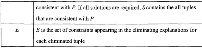
consistent with P. If all solutions are required, S contains the all tuples that are consistent with P.

E E is the set o f constraints appearing in the eliminating explanations for each eliminated tuple

Table 3-1 Notation of CDDBT

C onstraint-directed Dynamic B acktracking (CDDBT) Input: a CSP

Output: the first solution 1. P — 0

2. Ei •*- 0 for each i in I

3. W H ILE (P doesn’t covers vars AND (at least one constraint has not been chosen AND it contains a variable that is not assigned a value)) 4. Choose a constraint i from I where P doesn’t cover Vs involved variables 5. Ej — E i U s{P, i ) , S is obtained when calculating e(P, i)

6. IF (S <> 0 )

7. Choose a tuple t from S

8. Add (/, t) to P

9. ELSE

10. IF (E= 0 O R P = 0 )

11. RETURN No Solution

12. ELSE

13. Let (c, t) be the last entry in P that binds a constraint appearing in E if E <> 0 ; if not found, choose the last entry in P

14. Remove (c, t) from P

15. For each constraint k 'm P after c o r k not in P,

Remove from Ek any elimination explanation that involves c

16. Add (t, ~P) to Ec

17. END O F IF

18. END O F IF

Elim ination m echanism e (P ,i) :

1. tupleCanBeAdded false

2. W H ILE (tupleCanBeAdded = false AND at least one valid tuple cl in i has been chosen)

3. tupleAlreadylnEliminationExplanation false 4. tuplelsPermanentlyEliminated — false

5. IF (cl= t and (t, C) is an eliminating explanation of E,) 6. tupleAlreadylnEliminationExplanation *- tru e

7. IF (C = 0 )

8. tuplelsPermanentlyEliminated — tru e

9. END O F IF

10. END O F IF

11. tupleNeedsEliminating false

12. IF (tuplelsPermanentlyEliminated = false)

13. IF (P = 0 )

14. W H ILE (at least one cj in cks(P, i) has not been chosen)

15. IF (cl violates c/)

16. Add (cl, ci) to Et

17. tupleNeedsEliminating tru e

18. END O F IF

19. END O F W H ILE

20. ELSE

21. pseList — 0 , constraintList 0

22. W H ILE (at least on e (c, t) in P has not b een ch osen ) 23. Add (c, t) to pseList

24. Add c to constraintList

25. checkset cks(pses, i)

27. IF {cl violates t)

28. Add {cl, c) to Et

29. tupleNeedsEliminating *- tru e

30. ELSE

31. tup ■*- t U cl

32. W H ILE (at least one c/ in checkset has not been

chosen)

33. IF {tup violates c/)

34. Add {cl, c{) to Ei

35. tupleNeedsEliminating — tru e

36. END O F IF

37. END O F W H ILE

38. END O F IF

39. IF {{c, t) is not the first element in pseList)

40. IF {cl violates pscl)

41. Add {cl, constraintList) to E,

42. tupleNeedsEliminating ■*- tru e

43. ELSE

44. nppscl •*- pscl U cl

45. W H ILE (at least one c/ in checkset has not been

chosen)

46. IF {nppscl violates ci)

47. Add {cl, constraintList) to E,

48. tupleNeedsEliminating tru e

49. END O F IF

50. END OF W H ILE

51. END O F IF

52. END O F IF

56.

55. Add {cl, 0 ) to Ei

tupleNeedsEliminating tru e

57. END O F IF

58. END O F W H ILE

59. END O F W H ILE

60. END O F IF

61. END O F IF

62. IF (tupleAlreadylnEliminationExplanation = false AND

tupleNeedsEliminating = false)

63. Add cl to S

64. tupleCanBeAdded tru e

65. END O F IF

66. END O F W H ILE

3.3 Proof

Theorem 3.1: If a CSP is solvable, CDDBT can always retu rn a solution. Proof. Suppose we have a simple CSP:

Variables: V j,V2,...,V n

Domains: D /=D r=..-=D„= {di, d2,..., dh} Constraints: C/, C2,...,C m

We choose C/ first. We must find at least one tuple t/ from C/ that satisfies constraints

C2,...,C m because this CSP is solvable and elimination mechanism of CDDBT

eliminates any tuple before t2 that violates related constraints. If ti involves all

variables form V/ to V„, tj is a solution. If not, we choose the next constraint C* that involves at least one new variable. We look for a tuple t2 from Q that satisfies ti and related constraints. If we can not find it, we backtrack and look for another tj. We must find at least one tuple t2 from Q that satisfies tj and related constraints because this CSP is solvable and elimination mechanism of CDDBT eliminates any tuple

before tk that violates ti and related constraints. Then tj U 4 is a partial solution. If ti U

tk involves all variables form V/ to V„, tj U tk is a solution. If not, we choose the next constraint that involves at least one new variable. Following this procedure, we must find a solution.

3.4 An CDDBT Example

We use the same example as the example in CDBT: Given a simple CSP:

Variables: Vj, V2,..., V20

Domains: Di=D2-...= D2o- {1, 2, . . . , 30}

Constraints: C/, C2,...,Cg

Suppose we have already selected C/ and C2. So V/, V2, V3,and V4 have been assigned

4 Experiments

4.1 Random General CSP Generator

4.1.1 Methodology

At present, most random CSP generators are binary generators. Further more, they usually generate random CSPs with the same domain, the same arity, and the same tightness o f each constraint. They only generate random tuples o f each constraint. My random CSP generator is a general CSP generator and generates more random features. It generates a CSP with random variables, random domains, and random constraints.

In (Gent, MacIntyre, Prosser, Smith, & Walsh, 2001), the authors state that “many models o f random binary constraint satisfaction problems become trivially insoluble as problem size increases.” They claim that one reason for the problem is the appearance of “flawed variables” . Their definition of “flawed” is “A value for a variable is flawed if, when the value is assigned to the variable, there exists an adjacent variable in the constraint graph that cannot be assigned a value without violating the constraint between the two variables.” They also cite an early work by (Achlioptas et al., 1997), in which the authors prove that if tightness is larger than some value (related to domain size), as the problem size increases, the generated random binary CSP may have a flawed variable. My random general CSP generator may also suffer from this problem. Our concern in this thesis is CSP-solving algorithms, not random CSP models.

valid tuples of a constraint again and again. We call this the “unsuccessful hit” problem. We solve it using the following strategy. For example, if tightness ti is larger than 0.5, we first generate all possible tuples, then we generate invalid tuples with 1-

ti, finally we can easily obtain valid tuples.

My random general CSP generator has three modules:

generate random constraints generate random domains generate random variables

If we make this procedure more specific, that is:

generate random density

generate random domain o f each variable generate random number o f variables

generate random tightness of each constraint

generate random involved variables of each constraint

generate valid random tuples o f each constraint

remove constraints that violate the requirement o f arity and the requirement

4.1.2 A random CSP example

The output of my random general CSP generator is a CSP. The following is an example:

Arguments:

numberOfCSPsNeedsToBeGenerated=1

maximumNumberOfVariables=7

maximumDomainSize=4

maximumDensity=0.5

maximumArity=7

maximumTightnessOfConstraint=0.5

connected=true

randomLeve1=00000

******************^SP 0 has been Q^eneneted.*****************

numberOfVariables=5

Because argument maximumArity>numberOfVariables, maximumArity is

assigend to 5

VO's d o m a i n (1 elements): 0

Vi's d o m a i n (2 elements): 0 1

V 2 's d o m a i n (3 elements): 0 1 2

V 3 's d o m a i n (3 elements): 0 1 2

V 4 's d o m a i n (2 elements): 0 1

density=0.2242043106667143

numberOfAllPossibleConstraints=31

expected numberOfConstraints=6

cspIsConnected=true

C O 's involved v a r iables: V4

this constraint's tightness=0.4317 6073273825644

numberOfAllPossibleTuples=2

numberOfTAllowedTuples=l

< V 4 ,1>

C l 's involved v a riables: VI V3

this constraint's tightness=0.38900738448987093

numberOfAllPossibleTuples=6

numberO fTA11owedTup1e s=2

<V1,0> < V 3 ,0>

<V1,1> <V3,0>

C 2 's involved v a r iables: VO V2 V3 V4

this constraint's tightness=0.05772896162759178

numberOfAllPossibleTuples=l8

numberO f TAl1owedTup1e s=1

<V0,0> < V 2 ,1> <V3,1> <V4,1>

C3 ' s involved variables : VI V2 V4

this constraint's tightness=0.2511751603623239

numberOfAllPossibleTuples=12

numbe rO f TAl1owedTup1e s=3

<V1,0> < V 2 ,0> <V4,0>

<V1,1> <V2,2> <V4,1>

<V1,1> <V2,1> <V4,0>

C4 ' s involved variables: V0 VI V2 V4

numberOfAllPossibleTuples=12

numbe r0 f TAllowedTuples=3

<V0,0> <V1,1> < V 2 ,2> < V 4 ,1>

<V0,0> <V1,0> < V 2 ,1> < V 4 ,1>

<V0,0> <V1,1> <V2,0> < V 4 ,0>

C5's involved variables: VO V3 V4

this constraint's tightness=0.44465671147816943

numberOfAllPossibleTuples=6

numberOfTAl1owedTup1es=2

<V0,0> <V3,2> <V4,1>

4.2 Experiment Data

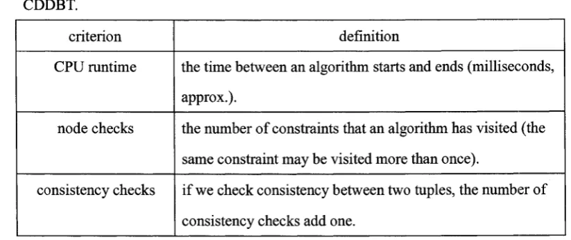
We are interested in how some CSP properties would influence the algorithms. These properties are number o f variables, size of each domain, density (or number of constraints), arity, and tightness o f each constraint. Three criteria (CPU runtime, node checks, and consistency checks) are used to evaluate the performance o f CDBT and CDDBT.

criterion definition

CPU runtime the time between an algorithm starts and ends (milliseconds, approx.).

node checks the number of constraints that an algorithm has visited (the same constraint may be visited more than once).

consistency checks if we check consistency between two tuples, the number of consistency checks add one.

Table 4-1 Three criteria for comparing the performance of CDDBT and CDBT

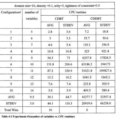
The generator can generate both connected and unconnected CSPs, but in this thesis only connected and solvable CSPs are used. Thirty CSPs are generated for each configuration (a configuration consists o f a given number of variables, a given domain size, density, arity, and tightness.) Then the average is put into the data tables. In the last three rows o f each table, AVG is average number. STDEV is sample

\ S ( X - X )

standard deviation, which is defined b y J —--- , where X is individual value, V n — 1

X is sample mean, and n is sample size (Bluman, 2001). Total Wins indicates the number that an algorithm has fewer CPU runtime, node checks, or consistency checks.

4.2.1 Target Property: number of variables

domain size=10, density =0.1, arity=3, tightness o f co n stra in ts.5

Configuration# number of

variables

CPU runtime

CDBT CDDBT

AVG STDEV AVG STDEV

1 5 2.8 3.6 7.2 18.8

2 6 3 3.3 35.7 50.6

3 7 4.6 5.4 110.1 196.9

4 8 10.8 10.8 523 921.8

5 9 34.3 73 6207.8 17824.5

6 10 131.8 206.6 63186.2 194173

7 11 87.2 320.9 31021.8 109827.6

8 12 13.2 10.2 1041.5 1665.2

9 13 7.6 7.4 233.8 305.9

10 14 5.9 5.9 409.5 589.4

AVG 9.5 30.1 64.7 10277.7 32557.4

STDEV 3.0 44.1 110.3 20919.6 66238.0

Total Wins 10 0

Table 4-2 Experiment #l(number of variables vs. CPU runtime)

domain size=10, density =0.1, arity=3, tightness of constraint=0.5

Configuration# number of

variables

node checks

CDBT CDDBT

AVG STDEV AVG STDEV

1 5 2.1 0.3 2.1 0.3

2 6 2.7 0.7 2.7 0.7

3 7 3.3 0.5 3.3 0.5

5 9 8.8 9.3 8.8 9.3

6 10 43 108.7 43 108.7

7 11 50.6 166.3 50.6 166.3

8 12 6.3 1.8 6.3 1.8

9 13 6.5 0.8 6.5 0.8

10 14 6.8 0.9 6.8 0.9

AVG 9.5 13.5 29.1 13.5 29.1

STDEV 3.0 17.8 58.8 17.8 58.8

Total Wins 0 0

Table 4-3 Experiment #l(number of variables vs. node checks)

domain size=10, density =0.1, arity=3, tightness o f constraint=0.5

Configuration# number of

variables

consistency checks

CDBT CDDBT

AVG STDEV AVG STDEV

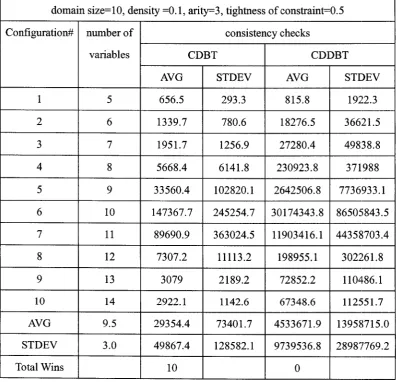
1 5 656.5 293.3 815.8 192.2.3

2 6 1339.7 780.6 18276.5 36621.5

3 7 1951.7 1256.9 27280.4 49838.8

4 8 5668.4 6141.8 230923.8 371988

5 9 33560.4 102820.1 2642506.8 7736933.1

6 10 147367.7 245254.7 30174343.8 86505843.5

7 11 89690.9 363024.5 11903416.1 44358703.4

8 12 7307.2 11113.2 198955.1 302261.8

9 13 3079 2189.2 72852.2 110486.1

10 14 2922.1 1142.6 67348.6 112551.7

AVG 9.5 29354.4 73401.7 4533671.9 13958715.0

STDEV 3.0 49867.4 128582.1 9739536.8 28987769.2

Total Wins 10 0

4.2.2 Target Property: domain size

number o f variables=10, density =0.1 , arity=3, tightness of constraint=0.5

Configuration# domain

size

CPU runtime

CDBT CDDBT

AVG STDEV AVG STDEV

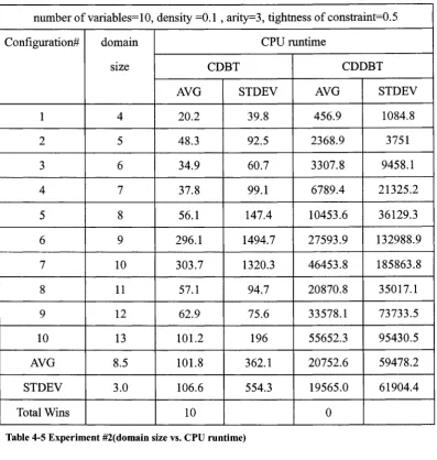
1 4 20.2 39.8 456.9 1084.8

2 5 48.3 92.5 2368.9 3751

3 6 34.9 60.7 3307.8 9458.1

4 7 37.8 99.1 6789.4 21325.2

5 8 56.1 147.4 10453.6 36129.3

6 9 296.1 1494.7 27593.9 132988.9

7 10 303.7 1320.3 46453.8 185863.8

8 11 57.1 94.7 20870.8 35017.1

9 12 62.9 75.6 33578.1 73733.5

10 13 101.2 196 55652.3 95430.5

AVG 8.5 101.8 362.1 20752.6 59478.2

STDEV 3.0 106.6 554.3 19565.0 61904.4

Total Wins 10 0

Table 4-5 Experiment #2(domain size vs. CPU runtime)

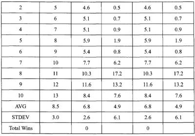
number o f variables=10, density =0.1, arity=3, tightness of co n strain ts. 5

Configuration# domain size node checks

CDBT CDDBT

AVG STDEV AVG STDEV

1 4 71.1 154.2 71.1 154.2