Junk, Veronika (2010): Hydrodynamical instabilities and the trace of dark energy within the CMB. Dissertation, LMU München: Fakultät für Physik

(1)

HYDRODYNAMICAL

I

NSTABILITIES AND

THE

TRACE OF

DARK

E

NERGY

WITHIN THE

CMB

(2)

(3)

HYDRODYNAMICAL

I

NSTABILITIES AND

THE

TRACE OF

DARK

E

NERGY

WITHIN THE

CMB

Dissertation

an der Fakult¨at f¨ur Physik der

Ludwig–Maximilians–Universit¨at (LMU) M¨unchen

Ph.D. Thesis

at the Faculty of Physics of the

Ludwig–Maximilians University (LMU) Munich

submitted by

Veronika Junk

from M¨unchen-Gr¨afelfing

(4)

(5)

1stEvaluator: Prof. Dr. Andreas Burkert 2nd Evaluator: Prof. Dr. Jochen Weller

(6)

(7)

Vorwort

Die Astrophysik beinhaltet und verknüpft verschiedene Bereiche der Physik, wobei interessante Prob-lemstellungen und fundamentale Sachverhalte (wie z.B. die Dunkle Energie) bis heute nicht eindeutig geklärt sind. Durch numerische Methoden gelingt es jedoch viele Prozesse, wie die kosmische Struk-turbildung, detailliert zu studieren. Da es in diesen Bereichen sehr viele interssante Fragestellungen gibt, habe ich mich in der vorliegenden Arbeit mit zwei Themen eingehend beschäftigt.

Die numerische Beschreibung von Strömungen und den dabei auftretenden Instabilitäten bildet die Grundlage für verschiedene hydrodynamische Prozesse in der Astrophysik. Um eine m öglichst genaue Darstellung der Entwicklung dieser Systeme zu erreichen, ist es wichtig an einem Testbeispiel die Genauigkeit der numerischen Algorithmen zu untersuchen. Der erste Teil meiner Dissertation be-fasst sich daher eingehend mit der Kelvin-Helmholtz Instabilität und deren numerische Umsetzung. Ein weiterer wichtiger Bereich der Astrophysik behandelt die Dunkle Energie, deren Eigenschaften und Ursprung. Da mich dieses Thema schon seit Beginn meines Studiums fasziniert, widme ich mich im zweiten Teil meiner Arbeit der Quantifizierung der Dunklen Energie mit Hilfe der kosmischen Hintergrundstrahlung.

(8)

(9)

List of Figures

1.1 KHI in nature . . . 2

1.2 Cosmological timeline part 1 . . . 3

1.3 WMAP sky map . . . 5

2.1 Basics scheme of Grid codes . . . 12

3.1 Shear flow initial configuration . . . 17

3.2 Time evolution of the linear analytical KHI growth . . . 21

3.3 Cloud in Cell: superimposed grid on SPH particles . . . 23

3.4 Time evolution of the KHI amplitudes with different resolution and different initial perturbation velocity . . . 25

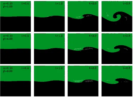
3.5 Evolution and growth of KHI for different AV-valuesα . . . 26

3.6 Evolution and growth of KHI for different AV-valuesβ . . . 27

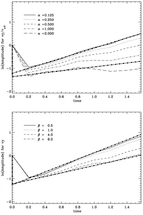
3.7 Time evolution of the KHI amplitudes with different values ofα andβ . . . 28

3.8 Time evolution of the KHI amplitudes with the Balsara-viscosity . . . 29

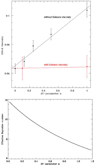
3.9 AV-parameterα versus the fitted viscosityνSPH . . . 30

3.10 Evolution and growth of the KHI for DC=10 . . . 31

3.11 Evolution and growth of the KHI for different DC . . . . 32

3.12 Time evolution of the KHI amplitudes for different DC . . . . 32

3.13 Time evolution of the KHI amplitudes for DC=10 using P08 . . . 33

3.14 Non-viscous time evolution of KHI amplitudes for equal density layers using FLASH and PLUTO in comparison to VINE, and viscous evolution using FLASH . . . 36

3.15 Non- and viscous time evolution of the KHI amplitudes for equal density layers using PROTEUS . . . 37

3.16 Analytical Slopes compared to the fitted slopes from FLASH and PROTEUS . . . . 39

3.17 Fitted viscosity (νnum) against physical viscosity (ν) using PROTEUS . . . 40

3.18 Evolution and growth of the KHI using FLASH and PLUTO for DC=10 . . . 42

3.19 Non-viscous time evolution of KHI amplitudes for DC=10 using FLASH, PLUTO and RAMSES . . . 43

3.20 Viscous time evolution of KHI amplitudes using FLASH for DC=10 . . . 44

3.21 FLASH, initial conditions using the ramp function to smooth the density contrast . . 45

(14)

4.1 Energy density contributions of the universe today . . . 50

4.2 Recipe of general relativity . . . 52

4.3 Evolution ofΩM,DEand D(z)for constant equation of states wDE=const. . . 64

4.4 Evolution of wDE,ΩM,DEfollowing the parameterization of LIND03 . . . 68

4.5 Evolution of D(z)following the parameterization of LIND03 . . . 69

4.6 Evolution of wDE,ΩM,DEfollowing the parameterization of KOMAT09 . . . 70

4.7 Evolution of D(z)following the parameterization of KOMAT09 . . . 71

4.8 Evolution of the wDE,ΩM,DEfollowing the parameterization of WETT04 . . . 73

4.9 Evolution of D(z)following the parameterization of WETT04 . . . 74

4.10 Components of power spectrum following PT at z=0 . . . 76

4.11 Power spectra using PT, MA99 and HALOFIT at the redshifts z=0, z=5 and 10 . . 82

4.12 Ratios of nonlinear to linear power spectrum using PT, MA99 and HALOFIT at the redshifts z=0 and 10 . . . 83

4.13 WMAP sky map . . . 84

4.14 Evolution of the primordial CMB temperature (CT T(l)), and polarization (CT E(l), CEE(l)) power spectrum with multipole-moment l . . . . 91

4.15 Evolution of ∂PΦ(k,z)/∂z with redshift for PT, MA99 and HALOFIT at constant wave numbers . . . 92

4.16 Evolution of ∂P_Φ(k,z)/∂z with redshift for PT, MA99 and HALOFIT at constant wave numbers . . . 93

4.17 Bispectrum amplitude|Q(l)_|with multipole-moment l for PT, MA99 and HALOFIT using wDE=−1. . . 94

4.18 Evolution of∂PΦ/∂z with redshift for k=0.04 MPC−1 . . . 95

4.19 Evolution of∂PΦ/∂z with redshift for k=0.4 MPC−1 . . . 96

4.20 Evolution of∂PΦ/∂z with redshift for l=100 . . . 97

4.21 Evolution of∂PΦ/∂z with redshift for l=1000 . . . 98

4.22 Evolution of∂PΦ/partialz with redshift for l=10000 . . . 99

4.23 Evolution of_|Q(l)_|with l for the DE models . . . . 100

4.24 Evolution of the bispectrum amplitude_|Q(l)_|and the bispectrum with the multipole-moment l for const. wDE, WETT04, LIND03 and KOMAT09 . . . 101

4.25 Evolution of S/N with lmaxusing constant equation of states wDE, WETT04, LIND03 and KOMAT09 . . . 102

4.26 Comparison of S/N with lmax . . . 103

5.1 KHI in nature . . . 107

A.1 FFT-Transformation of grid points . . . 128

A.2 Variation of KHI-amplitude for different values ofσ0 . . . 129

B.1 Test cases for the numerical integration method . . . 132

B.2 Comparison of D(z)using different DE-parameterizations . . . 133

B.3 Evolution of the comoving distance for different DE models . . . 134

B.4 Result for the ratio of nonlinear to linear power spectra following Giovi et al. (2003) 136 B.5 Evolution of dP_Φ/dz with redshift for k=4 MPC−1 . . . 138

(15)

LIST OF FIGURES xv

B.7 Evolution of S/N with lmaxusing constant equation of states wDE, WETT04, LIND03

(16)

(17)

List of Tables

3.1 Conversion of code units to physical units . . . 21

(18)

(19)

Zusammenfassung

Der erste Teil dieser Arbeit behandelt die numerische Beschreibung von Scherströmungen (grundlegend für astrophysikalische Prozesse auf verschiedensten Grössenskalen) und der dabei auftretenden Kelvin-Helmholtz Instabilität (KHI). Bezugnehmend auf die theoretische Herleitung von Chandrasekhar (1961), welche das lineare Wachstum der KHI erfasst, wird diese unter Mit-berücksichtigung der physikalischen Viskosität neu berechnet und bildet die Grundlage für spätere Anwendungen und Vergleiche mit numerischen Simulationen. Der numerische Teil stützt sich auf zwei weitverbreitete Methoden in der Astrophysik, ”Smooth-particle hydrodynamics” (SPH) und Gitter-Verfahren. SPH beschreibt eine Flüssigkeit durch Betrachtung von Teilchen, dessen Eigenschaften aus Nachbarteilchen innerhalb eines fest vorgegebenen Radiuses (der sogenannten Glättungs oder Smoothing Länge) bestimmt werden. Die in dieser Arbeit benutzten numerischen SPH-Algorithmen sind der VINE code (Wetzstein et al., 2009; Nelson et al., 2009) und der von Price (2008) (P08) beschriebene Code. Die intrinsische Viskosität in VINE wird mit Hilfe der analytischen Anwachsrate bestimmt, wobei der Effekt der sogenannten künstlichen Viskosität (wichtig in allen SPH-Anwendungen um Schock-Phänomene zu simulieren) analysiert wird. F ür die üblich angesetzen Parameter ist die Entwicklung der KHI in VINE erheblich gedämpft, was aber durch Verwendung der sogannten Balsara-Viskosität korrigiert werden kann. Im Fall unterschiedlicher Dichte der Strömungsschichten wird die KHI komplett unterdrückt. Dieses Problem, von numerischer Natur und daher in vielen SPH-methoden gegenwärtig, ist Mittelpunkt aktueller Forschung. Der von P08 entwickelte Code besitzt eine L ösung implementiert in Form einer künstlichen thermischen Konduktivität. Diese sorgt dafür, dass die thermische Energie, dessen Erhaltung ein Mischen der Teilchen verhindert, beim Übergang vom dichten ins dünne Medium ausgeschmiert wird und eine Mischung erm öglicht. Das gute Übereinstimmen des Vergleichs mit der analytischen Erwartung unterstützt diese Methode.

Die Gitterverfahren unterteilen eine Fl¨ussigkeit in Zellen, wobei die entsprechenden Gitterpunkte die gwichteten physikalischen Gr¨ossen beinhalten. Basierend auf den Gitter-codes FLASH (Fryxell

et al., 2000), PROTEUS (e.g. Heitsch et al., 2006), PLUTO (Mignone et al., 2007) und RAMSES

(20)

Der zweite Teil befasst sich mit der Thematik der Dunklen Energie (DE) und die Unterschei-dung verschiedener Modelle mit Hilfe der kosmischen Hingergrundstrahlung (CMB = ”cosmic microwave background”). Basierend auf den zwei weitverbreitesten Konzepten zur Charakter-isierung der DE, die kosmologische Konstante (wDE=−1) und die Quintessence (ein sich langsam

ver¨anderliches skalares Feld mit wDE 6= konst.) wird das theroretische CMB L-RS Bispektrum

berechnet. Es stellt eine Kreuz-Korrelation aus dem Rees-Sciama (RS) und dem Weak-lensing (L) Effekt dar. Die gravitative Ablenkung der CMB Photonen wird beschrieben durch den L-Effekt. Der RS-Effekt umfasst die späte Abnahme der Potential-Fluktuationen (Sachs & Wolfe, 1967) und das nichtlineare Wachstum kosmischer Strukturen (Rees & Sciama, 1968). Da das Wachstum beeinflusst wird von der DE geht hier direkt die Abhängigkeit vom entsprechenden DE-Modell ein. Besonderes von Interesse ist ein m öglicher Beitrag zu frühen Zeiten, beschrieben durch die sogenannte ”Early Dark Energy” (EDE). Um Vergleiche zu ziehen, werden zusätzlich zu EDE noch zwei weitere Quintessence-Modelle herangezogen, die Parameterisierung von Linder (2003a,b) (LIND03) und Komatsu et al. (2009) (KOMAT09), sowie Beispiele mit wDE=konst..

Weiterhin beinhaltet der RS-Effekt das lineare- wie das nichtlineare Wachstum von Dichtefluktu-ationen der sich bildenden Strukturen. Daher wird ein entsprechendes Modell zur Beschreibung des nichtlinearen Regimes benötigt. Auf Grundlage der kosmologischen Störungstheorie dritter Ordnung (PT) wird das von Bernardeau et al. (2002) vorgestellte Konstrukt benutzt. Um eine m ögliche Abhängigkeit der Resultate von diesen Modell zu quantifizieren werden (im Falle der kosmologischen Konstanten) die Beschreibungen von Ma et al. (1999) (MA99) und Smith et al. (2003) (HALOFIT) untersucht. PT und HALOFIT führen zu einer ähnlichen Entwicklung der L-RS Bispectrum-Amplitude. Der Übergang vom linearen in das nichtlineare Regime, deutlich durch den Vorzeichenwechsel der Amplitude, erreignet sich für MA99 auf grösseren Skalen im Gegensatz zu PT und HALOFIT. Dies lässt sich zurückführen auf den stärkeren nichtlinearen Beitrag von MA99 bei höhren Rotverschiebungen. Die Berechnung der Bispektrum-Amplitude für die verschiedenen Quintessence-Modelle beruht auf PT. Hierbei wird eine Abhängigkeit des Vorzeichenwechsels von dem Beitrag der DE deutlich. Je grösser die Dichte der DE, desto stärker wird das lineare Wachstum der Fluktuationen gedämpft, was ein späteres Erreichen der nichtlinearen Entwicklung zur Folge hat. Daher verschiebt sich der Übergang vom linearen in das nichtlinear Regime zu kleineren Skalen. Es ergeben sich deutliche Unterschiede der einzelnen Modellen, was sich auch in der Entwicklung des Signal-to-Noise Verhältnisses (S/N) wiederspiegelt. Das stärkste Signal folgt dem EDE-Modell mit

dem gr¨ossten DE-Beitrag. Durch Vergleich der S/N Entwicklung folgt, dass PLANCK die n¨otige

(21)

Summary

Given the importance of shear flows for astrophysical gas dynamics, we study the evolution of the Kelvin-Helmholtz instability (KHI) analytically and numerically. We derive the dispersion relation for the two-dimensional KHI including viscous dissipation. The resulting expression for the growth rate is then used to estimate the intrinsic viscosity of four numerical schemes depending on code-specific as well as on physical parameters. Our set of numerical schemes includes the Tree-SPH code VINE, an alternative SPH formulation developed by Price (2008), and the finite-volume grid codes FLASH, PROTEUS, PLUTO and RAMSES. In the first part, we explicitly demonstrate the effect of dissipation-inhibiting mechanisms such as the Balsara viscosity on the evolution of the KHI. With VINE, increasing density contrasts lead to a continuously increasing suppression of the KHI (with complete suppression from a contrast of 6:1 or higher). The alternative SPH formulation including an artificial thermal conductivity reproduces the analytically expected growth rates up to a density contrast of 10:1. The second part addresses the shear flow evolution with FLASH, PLUTO and RAMSES. All codes result in a consistent non-viscous evolution (in the equal as well as in the different density case) in agreement with the analytical prediction. The viscous evolution studied with FLASH shows minor deviations from the analytical prediction.

(22)

(23)

Chapter 1

Motivation

In this thesis, we study the implications of structure formation in an astrophysical context from two different perspectives. We start in the first part with the hydrodynamical evolution, where we play special attention to the occurring instabilities, in particular, the Kelvin-Helmholtz instability (KHI) and its implementation within numerical algorithms. In the second part, we analyze the effects of dark energy on forming cosmological structures (like galaxies), which leave a trace within the cosmic microwave background. 1.1 and 1.2, shortly motivate and introduce our further proceedings.

1.1 Part I : Modelling Shear Flows with SPH and Grid Based Methods

The physics of hydrodynamics are a central part in order to understand the evolution of astrophysical systems which involve any forms of gas. Therefore, structure formation at different scales can only be described sufficiently if the corresponding gas components are treated correctly. Very important in this context is the interstellar medium (ISM), which connects hydrodynamical processes on stellar-(small) and galactic-(large) scales. The ISM consists of_∼99% gas (mostly hydrogen and helium), and_∼1% dust made out of heavier elements (such as metals). On stellar scales, its dynamical evo-lution includes the turbulence of molecular clouds, which can be identified with the densest spots of the ISM. They provide the birthplaces for stars, which in turn fuel their surrounding with jets and outflows. On galactic scales, galaxy formation, where small subhalos (known as satellite galaxies) fall within the hot gaseous halo of its parent galaxy leads to an interaction between the satellites cold gas component and the ISM. Gas is stripped from the subhalo via ram pressure stripping1 and driven towards the center of the host galaxy, where the galactic disc formation takes place.

All these scenarious display a system known as shear flows, where two gas-layers move in the oppo-site direction. They play a crucial part in structure formation (see Fig. 1.2) and are fundamental to understand how the universe evolved into its form today. The various complex procedures are mod-eled by numerical methods, where smooth particle hydrodynamics (SPH) and grid based schemes are the most commonly used. Given the importance of shear flows and the corresponding instabilities for the evolution of cosmic structures, it is essential to verify how accurate numerical algorithms describe those systems, and to determine their limitations with a test example.

The KHI (see Fig. 1.1), arising from an oscillation of the interface between two fluid layers as a result of their velocity difference is important for several astrophysical processes where shear flows emerge.

(24)

Figure 1.1: KHI in nature: KHI forming in clouds (upper left panel), in earth’s atmosphere (upper right panel), and in Jupiters atmosphere (bottom panel).

It has given rise to serious discussion in the literature when numerically modeled. For example, its evolution is completely suppressed in presence of density contrasts when simulated with SPH (e.g. Agertz et al., 2007; Price, 2008). In contrast to this, grid codes seem to do not suffer from such a problem. But yet, it is not clear how exact they describe the evolution of this instability. We therefore focus on the incompressible KHI applying SPH and grid based codes in order to verify their depen-dency on numerical parameters and to test limitations and applications.

The outline is as follows:

• Chapter 2 introduces the theoretical framework necessary for chapter 3. The basic principles of hydrodynamics are discussed in section 2.1. A short introduction concerning the main features of SPH and grid codes is given in section 2.2.

(25)

1.2. PART II : THE TRACE OF DARK ENERGY CAPTURED WITHIN THE CMB 3

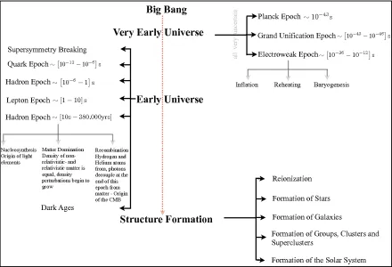
Figure 1.2: Cosmological timeline starting from the big bang until the formation of our solar sys-tem, see also Mukhanov (2005), Schneider (2006) or www.en.wikipedia.org/wiki/Timeline-of-the-Big-Bang).

growth is compared to the analytical expectation, where FLASH, PLUTO and RAMSES are in very good agreement. The summary of the results is presented in section 3.6.

1.2 Part II : The Trace of Dark Energy captured within the CMB

The surprising realization that our universe undergoes an accelerated expansion as accounted for by Supernova observations type Ia (SNIa) (Krauss & Turner, 1995; Ostriker & Steinhardt, 1995; Riess

et al., 1998; Perlmutter et al., 1999; Netterfield et al., 2002) is currently thought to originate from an

unknown energy density that fills up almost our complete universe today (∼70%). The origin and nature of this dark energy (DE) is one of the most challenging questions of astrophysics. Combined observations of SNIa, large scale structure (LSS) (Colless, 1999; Abazajian et al., 2003) and the cosmic microwave background (CMB) (Spergel et al., 2003; Komatsu et al., 2009) point toward an equation of state2for DE which is close to wDE≈ −1. The standard picture invokes a cosmological

constant (Λ) with the energy density of the vacuum. Yet, there exist also other possibilities like

2 _{The ratio of pressure to density w}

(26)

models with a time varying wDE. A very common branch of these approaches is based on particle

physics, which describe DE via a slowly changing scalar field called the quintessence. Its behavior at late times adapts that ofΛ with wDE=−1, but differs from this in the past. Several attempts have been

discussed, where certain parameterizations of wDEencompass a range of models. The only possibility

to distinguish between different approaches and to constrain further parameters of DE is provided by observations, where among SNIa- and LSS measurements the CMB plays an important role.

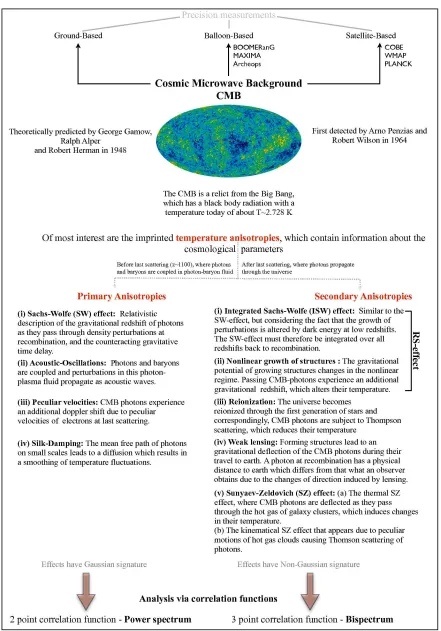
The CMB, a relict from the big bang results from the decoupling of matter and radiation at the epoch of recombination (see Fig. 1.2). It presents the most accurate measured black body radiation (Penzias & Wilson, 1965) with a temperature today about T_∼2.728 K. In particular, the imprinted anisotropies (see Fig. 1.3), induced through interactions of CMB photons with their surrounding environment allow to gain insight into the physics at early times and to constrain cosmological parameters. The primary anisotropies arise before the CMB photons have decoupled and leave a Gaussian signature within their temperature distribution. However, for our study the secondary anisotropies are of more interest. These are caused as the photons travel through the universe after decoupling and interact with the forming structures. Since DE influences the growth of density fluctuations, the CMB photons carry information about DE and its equation of state wDE. This is described by the Rees-Sciama (RS) effect

(see also Fig. 1.3). It leaves, along with gravitational deflection (weak lensing) a non-Gaussian signal within the CMB.

The CMB bispectrum, a tool to analyze non-Gaussianity is therefore useful to constrain properties of DE. The focus of the second part of this work is thus on the cross correlation bispectrum between the weak lensing- and RS-effect (L-RS bispectrum). We calculate the theoretical L-RS bispectrum and the corresponding signal to noise ratio using different models of DE. They aim is to obtain the limits of future CMB-observations to distinguish betweenΛ and quintessence. The outline is as follows:

• In Chapter 4 we concentrate on the calculation of the L-RS bispectrum and the signal-to-noise ratio(S/N). We start with an introduction followed by a short recap of cosmological basics in section 4.2, fundamental for this work. In section 4.3 we motivate the DE-models with constant

wDE and the quintessence models following Wetterich (2004) (WETT04), Linder (2003a,b)

(LIND03) and Komatsu et al. (2009) (KOMAT09), respectively. Section 4.4 introduces the description of the nonlinear power spectrum using Bernardeau et al. (2002) (PT), the model of Ma et al. (1999) (MA99) and Smith et al. (2003) (HALOFIT), respectively. The basics of CMB correlation-functions are given in section 4.5. The L-RS bispectrum is discussed in detail in section 4.6, using PT, MA99 and HALOFIT, as well as the DE-models with constant wDE,

WETT04, LIND03 and KOMAT09. The S/N evolution follows in section 4.7. We conclude

with section 4.8

(27)

1.2. PART II : THE TRACE OF DARK ENERGY CAPTURED WITHIN THE CMB 5

(28)

Theoretical Basics

In this chapter we present the theoretical background required in chapter 3. First, the hydrodynamical principles and the linear perturbation theory are introduced. This provides the framework to derive the analytical growth rate of the Kelvin-Helmholtz instability carried out in section 3.2. Afterwards, the characteristic properties of our numerical algorithms - Smooth Particle Hydrodynamics (SPH) and grid based codes - are briefly discussed.

2.1 Basics of Hydrodynamics and Instabilities

This short overview mostly uses the convention given in Landau & Lifschitz (1991), where a complete introduction to hydrodynamics can be found.

2.1.1 Equation of Motion for the Fluid

The state of a fluid is determined by five quantities: the three velocity components (v), the density (ρ) and the pressure (p). It experiences additional transfer of momentum due to internal friction forces, resulting in a relative motion between the different fluid-layers. This is expressed by the momentum flux density tensor (Π), written in its components,

Πik=ρvivk−σik, (2.1)

whereρ is the density of the fluid and vi, vkthe corresponding velocity components. The quantityσik

represents the stress tensor,

σik=−pδik+σik′, (2.2)

with p being the pressure, δikthe kronecker-symbol (that equals 1 if i=k, and 0 otherwise), and σik′

the viscous stress tensor, which is a linear function of the first spatial velocity derivatives (Landau & Lifschitz, 1991).

The motion for this kind of fluid is fully described by the Navier-Stokes equation,

ρ· ∂

v

∂t + (v·∇)v

=₋∇p₋ρ∇φ+η_△v+ξ+η

3

(29)

2.1. BASICS OF HYDRODYNAMICS AND INSTABILITIES 7

with the gravitational potentialφ, and the constant viscous coefficients η andξ. For an incompress-ible fluid, which implies no sources (∇_·v=0), the last term in eq. (2.3) vanishes and the equation simplifies to,

ρ· ∂

v

∂t + (v·∇)v

=₋∇p₋ρ∇φ+ρν_△v. (2.4)

Here we introduced the kinematical viscosityν, ν=η

ρ. (2.5)

The mass conservation is expressed by the continuity equation, ∂

∂tρ+∇(ρ·v) =0. (2.6)

If the fluid does not have inherent viscosity (ν=0), we obtain the familiar Euler-Jeans-equation, ρ·

∂ v

∂t + (v·∇)v

=₋∇p₋ρ∇φ. (2.7)

To fully determine the fluid properties, we also need the equation of state,

p=p(ρ,S), (2.8)

where S expresses the entropy. The equation of state is the link between thermodynamics and hydro-dynamics. For example, the equation of state for a isothermal ideal gas is given by,

p= nRT

V , (2.9)

where R denotes the gas constant1, n=N/ρ the particle density and T the temperature.

2.1.2 Hydrodynamical Instabilities in the Linear Regime

To mathematically describe the perturbations leading to instability effects we apply the first order perturbation theory. The perturbed values of the fluid are given by,

v _→ v+δv, (2.10)

ρ → ρ+δρ, (2.11)

p _→ p+δp. (2.12)

δv expresses the perturbation in the velocity,δρ andδp in the density and pressure, respectively. For

the linearized Navier-Stokes- and continuity equation follows, ρ(∂tδv+ (v·∇)δv+ (δv·∇)v) +δρ(∂tv+ (v·∇)v) =

−∇(δp) +ρν_△δv+δρν_△v+ρ∇(δφ) +δρ∇φ, (2.13)

∂tδρ+ (v·∇)δρ+ (δv·∇)ρ=0, (2.14)

where we use the abbreviation ∂/∂t :=∂t. Eq. (2.13), and eq. (2.14) are crucial to derive the growth

rate of the Kelvin-Helmholtz instability, which is discussed in detail in Chapter 3, section 3.2. They also provide the fundament of treating linear cosmological perturbations in the Newtonian limit dis-cussed in Chapter 4, section 4.2.6.

(30)

2.2 Numerical Methods

Numerical algorithms are an important tool in modern astrophysics. Their ability to follow linear as well as nonlinear dynamics provides a detailed insight into complex physical processes. To treat hydrodynamical systems, two basic approaches are widely used: SPH and Grid-based codes.

The equations of fluid dynamics (eq. (2.4), and eq. (2.7)) have the form

dv dt =

∂

∂t+ (v·∇)

v= f(v,∇_·v,r), (2.15)

where the convectional derivative is defined by

d dt :=

∂

∂t+ (v·∇)

. (2.16)

Eq. (2.15) can be interpreted as

dA

dt = f(A,∇A,r), (2.17)

where A characterizes any physical quantity. To determine the rates of change of physical quantities requires their spatial derivatives. In numerical simulations, any algorithm approximates these deriva-tives using information from a finite number of points. In Grid-codes, the points are identified with the vertices of a mesh (see 2.2.2). For SPH, the interpolating points are the particles moving with the flow, and the interpolation of any quantity is based on a kernel estimation (see 2.2.1). In the following both approaches are introduced.

2.2.1 Basic Principles of SPH-codes

We outline shortly the basic assumptions and equations of SPH. A detailed introduction to SPH can be found in Monaghan (1992, 2005), Benz (1990) and references therein. The original idea dates back to Gingold & Monaghan (1977) and Lucy (1977).

• Interpolation and SPH equations:

SPH follows the equations of fluid dynamics using a set of particles. It presents a ker-nel estimation technique, where the value of a general function A(r) at some specific point (particle) is estimated by ’smoothing’ over the values of this function at neighboring particles. The integral interpolation (Aint) of any function A(r)is defined as

Aint(r) =

Z

A(r′)W(r₋r′,h)dr′, (2.18)

where h is the smoothing length that determines the region for contributing neighbors and dr′ a differential volume element. W characterizes an interpolation kernel, which must satisfy two properties:

Z

W(r₋r′,h)dr′:=1, (2.19)

lim

h→0W(r−r

(31)

2.2. NUMERICAL METHODS 9

The function A is reproduced exactly if the kernel is a delta function, while the normalization to 1 guarantees that also constants are interpolated exactly. In most numerical applications the kernel has a Gaussian form, W(r₋rb,h)∼exp[−(r−rb)2/h2]. This produces a symmetric

central force between pairs of particles, thereby conserving linear and angular momenta. A more convenient choice to ensure a finite range kernel (fixed number of neighbors) is based on a cubic spline (Monaghan & Lattanzio, 1985),

W(r,h) = τ

hκ·f

r h =   

1₋3₂q2+₄3q2 0_≤q<1,

1 4(2−q)

2 ₁_≤_q_<₂_,

0 q_≥2,

(2.21)

with q=r/h, andτ= [2/3; 10/(7π); 1/π]for theκ=1,2,3 spatial dimensions. For numerical studies, eq. (2.18) can be approximated by a summation interpolant,

Asum(r) =

∑

b

mb

Ab

ρb

W(r−rb,h), (2.22)

where the sum goes over all particles (indicated by summation index b), with the physical quantities beingρb, mb, vb, rb, Ab. For example, the density is defined as,

ρ(r) =

∑

b

mbW(r−rb,h). (2.23)

Provided that the kernel is differentiable it follows,

∇Asum(r) =

∑

b

mb

Ab

ρb

∇W(r₋rb,h). (2.24)

However, the derivative does not vanish if A is constant. To ensure this, we have to write (Monaghan, 2005),

∇A= 1

Φ(∇(ΦA)−A∇Φ), (2.25)

whereΦ is a differentiable function. This results in, ∇Asum=

1 Φa

∑

mb

Φb

ρb

(Ab−Aa)∇aWab, (2.26)

where∇aWabis the gradient of W(ra−rb,h)with respect to particle a. Eq. (2.26) vanishes if A

is constant.

Various forms of Φ exist, resulting in different versions of derivatives. For example, using Φ =ρ we can write the continuity equation (eq (2.6)2) either as

dρa

dt =ρa

∑

_b mb

ρb

vab·∇aWab, (2.27)

or

dρa

dt =

∑

_b mbvab·∇aWab, (2.28)

(32)

where vab=va−vb, respectively. Comparing eq. (2.27) with eq. (2.28), we see that the former

involves ρ explicitly, while the latter does not. This can be crucial if systems with different (fluid) densities are involved. If this is the case, then eq. (2.27) is more accurate. Near an inter-face the summation for, e.g.∇_·v involves contributions of both fluids. Using the summation of eq. (2.27), the ratio of mass to density will be constant and∇_·v remains unchanged (Colagrossi, 2004). However, using that of eq. (2.28) the mass elements change and the estimate of∇_·v will be different, even if the fluids have the same velocity and particle positions and differ only in the density. Monaghan (2005) states that for density contrasts_≤2 both descriptions are valid, but for larger contrasts eq. (2.27) is preferred. We return to this important point in chapter 3 under section 3.4.

For the pressure gradient follows,

∇p ρ =∇ p ρ + p

ρ2∇ρ, (2.29)

and the momentum equation3becomes,

dva

dt =−

∑

_b mb

Pb

ρ2

b

+Pa

ρ2

a

∇aWab. (2.30)

Eq. (2.30) can be derived from a discrete form of the action principle of an adiabatic fluid, it is symmetric and conserves linear and angular momentum, see Monaghan (1992).

The thermal energy per unit mass (u) is determined by the first law of thermodynamics

du=T dS₋pdV =T dS+ p

ρ2dρ, (2.31)

with S being the entropy. For the derivative of u follows

du dt =

p

ρ2

dρ dt =−

p

ρ∇·v, (2.32)

where we use the continuity equation of the form dρ/dt=₋ρ(∇_·v). Applying the different SPH descriptions (eq. (2.27), and eq. (2.28)), this expression transforms either into,

du dt =

Pa

ρ2

a

∑

b

mbvab·∇aWab, (2.33)

or

du dt =

Pa

ρa

∑

_b

mb

ρb

vab·∇aWab, (2.34)

respectively. It can be useful to treat the energy in SPH in terms of the thermokinetic energy per unit mass,

e=1

2v

2₊_u_, _(2.35)

(33)

which evolves according to,

de dt =−

1

ρ∇(p·v) =−

∑

_b mb

pavb

ρ2

a

+pbva

ρ2

b

∇aWab, (2.36)

and is symmetric like eq. (2.30). The description of the thermokinetic energy is often used in shock phenomena modeled with grid schemes, since it guarantees the conservation of energy.

• Artificial viscosity in SPH:

Artificial viscosity (AV) is not a real physical viscosity. It is implemented in order to permit the treatment of shock phenomena. Eq. (2.30) does not allow for dissipation of kinetic energy into heat, and therefore cannot describe shock features. In nature, the always present intrinsic viscosity of the fluid regulates this dissipation. In SPH this is done by adding an completely artificial viscosity term and modifying the equations of momentum and energy conservation correspondingly. Monaghan & Gingold (1983) present an example for AV based on simple arguments referring to its form and relation to gas viscosity. A viscous term,Πab4is

added to the SPH-evolution equation for the velocity (eq. (2.30)),

dva

dt =−

∑

_b mb

pb

ρ2

b

+ pa

ρ2

a

+Πab

∇aWab, (2.37)

where,

Πab=−ν

vab·rab

r2

ab+ε¯h2ab

. (2.38)

The quantityε_∼0.01 prevents a singularity if rab→0, while forνfollows,

ν=α¯habc¯ab

¯ ρab

, (2.39)

¯hab= (ha+hb)/2 and ¯cab= (ca+cb)/2, c denotes the sound speed. Πabis Galilean invariant

and leads to a repulsive force when two particles approach each other, where it acts as an attractive force if they are receding. An improved form which prevents the so called particle streaming (i.e. particles belonging to different areas streaming between each other) leads to (Monaghan, 1992),

ν= ¯hab

¯ ρab

αc¯ab−β

¯habvab·rab

r2_ab+ε¯h2

ab

, (2.40)

cab=ca−cb is the difference of the sound speeds. The first term ∼¯hab/ρ¯abαc¯ab can be

in-terpreted as a kind of shear and bulk viscosity, whereα controls its strength. The second term ∼¯hab/ρ¯abβ

¯habvab·rab/ r2ab+ε¯h2ab

resembles the von Neumann-Richtmyer viscosity, con-trolled byβ. It becomes important if compression arises. The form of eq. (2.40) has evolved further, see Lattanzio et al. (1985). Best results are achieved with the AV-parametersα=1 and β =2, but see for a more detailed study of their effects chapter 3, section 3.4.

(34)

x(j+1) x t t(n−1) t(n) t(n+1) x(j−1) x(j)

Figure 2.1: The grid discretizes the fluid in time and space (shown here by the x-direction).

Due to the AV term, energy is transformed from kinetic to thermal energy. Therefore, its con-tribution must also be added to the thermal energy equation (eq. (2.33)) correspondingly. The final result is given by (Monaghan & Gingold, 1983; Monaghan, 1997)

du dt =

pa

Ωaρa2

∑

b

mbvab·∇aWab+

1

2

∑

_a ma

∑

_b mbΠabvab·∇aWab. (2.41)

For the thermokinetic energy (eq. (2.36)) an dissipative term of the form

ϒab=−

Kvsig(a,b) e∗a−e∗b

ˆr ¯

ρab

, (2.42)

has to be added, where

e∗_a=1

2(va·ˆr)

2

+ua, (2.43)

and ˆr=rab/|rab|. vsigis the signal velocity and K is a constant. Eq. (2.36) generalizes to,

dea

dt =−

1

ρ∇(p·v) =−

∑

_b mb

pavb

ρ2

a

+pbva

ρ2

b

+ϒab

∇aWab. (2.44)

2.2.2 Basic Principles of GRID-codes

Another very promising and widely used approach to solve the hydrodynamical equations is presented by the Grid-codes. In this framework, various methods to solve the differential equations in terms of grid points have been proposed.

All grid-methods divide the fluid into separate cells called the mesh. An example is shown in Fig. 2.1. A common scenario to solve partial differential equations, in particular the fluid equations (eq. 2.15) is known as discretization, while a further improvement is provided by the Riemann-Solvers. We motivate both approaches below:

• DISCRETIZATION METHODS: A very simple method is to transform the regarded equations

into an discretized form. For example, consider the one-dimensional scalar equation ∂A

∂t +b

∂A

(35)

where b is a positive constant. We seek the solution A(x,t), with the following initial conditions,

A(x,0) =Ψ(x). (2.46)

Assuming that the mesh spacing ∆x, and the time step∆t are constant, the solution A(x,t)can be expressed by the analogous discretized solution at the mesh cell j and time level n as An_j, which is located at the center of the cell in physical space (see also Fig. 2.1). By replacing the derivatives of eq. (2.45) with one-sided finite difference approximations the equation becomes,

An_j+1₋An_j

∆t +O(∆t) +b

An_j₋An_j₋₁

∆x +O(∆x) = 0 for b>0 (2.47)

An_j+1₋An_j

∆t +O(∆t) +b

An_j₊₁₋An_j

∆x +O(∆x) = 0 for b<0. (2.48)

This scenario applies the one-sided forward differencing in time. Depending on whether b is positive or negative, the left side of the grid point j is called upwind side for b>0 (downwind side for b<0), while the right is called downwind side for b>0, (upwind side for b<0). If the error terms are dropped, the discrete evolution equation for An

j follows as,

An_j+1 = An_j+b∆t

∆x A

n j−1−Anj

for b>0, (2.49)

An_j+1 = An_j+b∆t

∆x A

n j−Anj+1

for b<0, (2.50)

where the term b_∆∆_xt determines the stability of the scheme, and is called CFL (Courant, Friedrichs, and Lewy) number. The scheme is stable, if

b∆t

∆x

≤

1. (2.51)

There exist various simple finite difference schemes, e.g. downwind differencing or centered differencing.

• RIEMANN SOLVERS: These schemes are used to solve Riemann problems (RP), such as the

hydrodynamical fluid equations. The RP’s are fundamental to study the interaction between waves, and allow to analyze the micro-wave structure of the flows. Properties like shocks and rare-fraction waves appear as characteristics in the solution. RP’s consist of conservation laws together with piecewise constant data including a single discontinuity. Thus, they appear naturally in grid codes, which solve conservation laws on discrete grids.

For example, a simple, one dimensional RP has the initial state of,

A(x,0) =

AL for x≤0,

AR for x>0,

(2.52)

(36)

system begins to evolve5_.

For the Euler equations (eq. (2.7)), the RP is defined as:

ρ,v,P=

ρL,vL,PL for x≤0,

ρR,vR,PR for x>0, (2.53)

It is much more complex due to the nonlinear nature of eq. (2.7). Analytical solutions can be obtained only for special cases. The majority of RP’s are solved numerically.

The first exact numerical solver was introduced by Godunov (1959). It is an extension to the discretization method (as discussed above) for solving nonlinear-systems of hyperbolic conser-vation laws. Consider Fig. 2.1 with the numerical solution at tn given by Anj, which is located

at the cell-center xj. The interface between two cells resides at xj+1/2. At each time step the

state within each cell is constant (piecewise constant). Yet, at the interfaces the state variables describe a jump. This construct resembles the definition of a RP, here within two adjacent cells. The solution at each interface characterizes the subgrid analytic evolution of the hydrodynamic system.

Based on Godunovs-Theorem (Godunov, 1954), which states that linear numerical schemes that are used to solve partial differential equations are first-order accurate, various methods of ap-proximate solvers have been proposed, e.g. Roe solver (Roe, 1981), HLLC solver (Harten et al., 1983), HLLE solver (Harten et al., 1983; Einfeld, 1988), and Rotated-hybrid Riemann solvers (Nishikawa & Kitamura, 2008).

5 _{These so called shock tube tests are very common to test the accuracy of numerical hydrodynamical schemes (e.g. Sod,}

(37)

Chapter 3

Modelling Shear Flows with SPH and

Grid Based Methods

3.1 Introduction

3.1.1 Definitions:

In general, shear flows express two fluid- or gas-layers, which are moving in the opposite direction. They are an integral part of many astrophysical processes, from jets, the formation of cold streams, to outflows of protostars (Dekel et al., 2009; Agertz et al., 2009; Diemand et al., 2008; Walch et al., 2010), and cold gas clouds falling through the diffuse hot gas in dark matter halos (Bland-Hawthorn

et al., 2007; Burkert et al., 2008). Jets and outflows of young stars can entrain ambient material,

leading to mixing and possibly the generation of turbulence in e.g. molecular clouds (Burkert, 2006; Banerjee et al., 2007; Gritschneder et al., 2009b; Carroll et al., 2009), while the dynamical interaction of cold gas clouds with the background galactic halo medium can lead to gas stripping of e.g. dwarf spheroidals (e.g. Grcevich et al., 2010), and the disruption of high-velocity clouds (Quilis & Moore, 2001; Heitsch & Putman, 2009). The KHI, arising from an oscillation of the interface between two fluid layers as a result of their velocity difference is believed to significantly influence the gas dynam-ics in all of these different scenarios.

Moreover, viscous flows play a crucial role in e.g. gas accretion onto galactic discs (Das & Chattopad-hyay, 2008; Park, 2009; Heinzeller et al., 2009), as well as in dissipative processes like the turbulent cascade. Typically, the gas viscosity seems to be rather low in the interstellar medium, with typical flow Reynolds numbers of 105.

(38)

contact discontinuities, or velocity gradients occurring in e.g. shear flows (see Agertz et al., 2007), thus suppressing shear instabilities such as the KHI.

3.1.2 Earlier Studies:

An interesting problem to test the limitations of SPH as well as grid codes is the passage of a cold dense gas cloud moving through a hot and less dense ambient medium (Murray et al., 1993; Vietri

et al., 1997; Agertz et al., 2007). Such a configuration would be typical for gas clouds raining onto

galactic protodisks, for High-Velocity Clouds in the Milky Way and for cold HI clouds in the Galactic disk. Murray et al. (1993) demonstrated using a grid code that in the absence of thermal instabilities and/or gravity clouds moving through a diffuse gas should be disrupted by hydrodynamical shear flow instabilities within the time they need to travel through their own mass. Agertz et al. (2007) have shown that the KHI, and therefore the disintegration of such clouds is suppressed in SPH simulations. This problem, in particular the suppression of the KHI, has been subject to recent discussion in the literature. Several solutions have been proposed, e.g. Price (2008) discusses a mechanism, which involves a special diffusion term (see also Wadsley et al., 2008).

Furthermore, Read et al. (2010) identify two effects occurring in the SPH formalism, each one sepa-rately contributing to the instability suppression. The first problem is related to the leading order error in the momentum equation, which should decrease with increasing neighbor number. However, nu-merical instabilities prevent its decline. By introducing appropriate kernels, Read et al. (2010) showed that this problem can be cured. The second problem arises due to the entropy conservation. Entropy conservation inhibits particle mixing and leads to a pressure discontinuity. This can be avoided by using a temperature weighted density following Ritchie & Thomas (2001). Recently, Abel (2010) has shown to reduce the leading error problem by using a novel discretization of the pressure equation, which smoothes the force on the kernel scale and improves the stability.

Another characteristic of SPH is the implementation of an artificial viscosity (AV) term (Monaghan & Gingold, 1983), which is necessary in order to treat shock phenomena and to prevent particle in-terpenetration. AV can produce an artificial viscous dissipation in a flow corresponding to a decrease of the Reynolds-number and therefore a suppression of the KHI (Monaghan, 2005). To confine this effect, a reduction of viscous dissipation was proposed by Balsara (1995) and improved by Colagrossi (2004). Thacker et al. (2000) studied different AV-implementations in SPH and pointed out that the actual choice of the AV-implementation is the primary factor in determining code performance. An extension of SPH which includes physical fluid viscosities was discussed by e.g. Takeda et al. (1994), Flebbe et al. (1994), Espa˜nol & Revenga (2003), Sijacki & Springel (2006) and Lanzafame et al. (2006).

An alternative to conventional numerical schemes may arise from a new class of hybrid schemes based on unstructured grids and combining the strengths of SPH and grid codes (Springel, 2010). Some of the problems listed above might be solved with this type of implementation.

3.1.3 Outline:

(39)

3.2. KHI – ANALYTICAL DESCRIPTION 17 s 0000000000000000000000 0000000000000000000000 0000000000000000000000 0000000000000000000000 0000000000000000000000 0000000000000000000000 0000000000000000000000 0000000000000000000000 0000000000000000000000 0000000000000000000000 1111111111111111111111 1111111111111111111111 1111111111111111111111 1111111111111111111111 1111111111111111111111 1111111111111111111111 1111111111111111111111 1111111111111111111111 1111111111111111111111 1111111111111111111111 0000000000000000000000 0000000000000000000000 0000000000000000000000 0000000000000000000000 0000000000000000000000 0000000000000000000000 0000000000000000000000 0000000000000000000000 0000000000000000000000 1111111111111111111111 1111111111111111111111 1111111111111111111111 1111111111111111111111 1111111111111111111111 1111111111111111111111 1111111111111111111111 1111111111111111111111 1111111111111111111111 ρ U

U1 ρ1

2 2 x z Fluid−layers Interface layer at z=z

Figure 3.1: Sketch of the initial conditions considered: Two fluid layers with constant densitiesρ1and

ρ2flowing in opposite directions with uniform velocities U1and U2.

on the standard SPH implementation, which does not contain a physical viscosity but instead uses AV. However, as mentioned above, AV does influence the evolution of the flow. In section 3.4, we discuss the ability of two numerical SPH-schemes to model the incompressible KHI, namely the Tree-SPH method VINE (Wetzstein et al., 2009; Nelson et al., 2009), and the SPH code of Price (2008). By comparing to the derived analytical solution, we asses the effects of AV in VINE and estimate the intrinsic physical viscosity caused by AV (3.4.1). We then study the development of the KHI for different density contrasts (3.4.2). We show that the instability is suppressed for density contrasts equal to or larger than 6 : 1. We also discuss the remedy suggested by Price (2008), hereafter P08. In section 3.5 we then study the same problem with the grid codes, FLASH (Fryxell et al., 2000), PROTEUS (e.g. Heitsch et al., 2006), PLUTO (Mignone et al., 2007) and RAMSES (Teyssier, 2002). We study the non-viscous as well as the viscous evolution of the KHI for equal (3.5.1) as well as non-equal (3.5.2) density layers. We summarize our findings in section 3.6.

3.2 KHI – analytical description

The Kelvin Helmholtz instability is a very common phenomena. It might be found either for fluid-layers with a sufficient difference in the velocity across their interfaces, or in a continuous fluid, if a form of velocity shear is present. Considering two incompressible fluid layers (Fig. 3.1) with constant densities (ρ1,ρ2), and flow velocities (U1, U2) an external perturbation results in an oscillation of the

interface, where the amplitude grows due to a pressure difference between concavities and convexities of the oscillation. This leads to a rolling up of the boundary layer. An example is the flow of air over water, responsible for the buildup of waves.

To derive the growth rate of the KHI including viscosity, we follow the analysis of Chandrasekhar (1961) (see also Funada & Joseph (2001) and Kaiser et al. (2005)). The fluid system is assumed to be viscous and incompressible. We use Cartesian coordinates in x, y, and z with two fluids at densities ρ1,ρ2, and velocities U1, U2 moving antiparallel along the x-axis, separated by an interface layer at

z=zs, see Fig. 3.1. We neglect the effect of self-gravity. The hydrodynamical equations for such a

(40)

3.2.1 Linear Perturbations

This analysis is an extension of the work done by Chandrasekhar (1961), where we rederive the linear KHI growth including a constant viscosity. The linearized Navier-Stokes- (eq. (2.3)) and continuity-equation (eq. (2.6)) are determined by eq. (2.13) and eq. (2.14). The perturbed quantities are given by,

v _→ v+δv, (3.1)

ρ → ρ+δρ, (3.2)

p → p+δp, (3.3)

where v= (U(z) +u,v,w) with u,v,w expressing the perturbation in the velocity and δρ, δp in

the density and pressure, respectively. The goal of this calculation is the dispersion-relation, which contains the time evolution of the modes and allows to constrain the linear KHI growth rate.

Inserting these perturbed values into eq. (2.13) and eq. (2.14) yields the system of linearized equations as

ρ∂tu+ρU∂xu+ρw∂zU = −∂xδp+ν(ρ+δρ)∂z2U+ρν(∂x2+∂y2+∂z2)u, (3.4)

ρ∂tv+ρU∂xv = −∂yδp+ρν(∂x2+∂y2+∂z2)v, (3.5)

ρ∂tw+ρU∂xw = −∂zδp+ρν(∂x2+∂y2+∂z2)w+

∑

s

Ts

(∂_x2+∂_y2)δzs

·δ(z₋zs), (3.6)

∂tδρ+U∂xδρ = −w∂zρ, (3.7)

∂tδzs+Us∂xδzs = −w(zs), (3.8)

∂xu+∂yv+∂zw = 0. (3.9)

Eqs. (3.4), (3.5) and (3.6) represent the linearized Navier-Stokes equation, where in eq. (3.6) the effect of surface tension has been incorporated, and the density may change discontinuously at the interface positions denoted by zs. The derivatives ∂/∂t,x,y,z are abbreviated by ∂t,x,y,z. Tsis introduced as an

advanced parameter who describes the surface tension at the shear layer. It does not play a role for our analysis, yet to be complete we include it in the calculation. Eq. (3.7) is the linearized continuity equation. In eq. (3.8) the subscript s distinguishes the value of the quantity at z=zs (the interface

layer). The last equation, eq. (3.9) expresses the incompressibility of the fluid. With perturbations of the form

u,v,w,δρ,δp,δzs∼exp[i(kxx+kyy+nt)], (3.10)

where D_≡d/dz and k2=k_x2+k2_y, we arrive at

iρ(n+kxU)u+ρ(DU)w = −ikxδp−ρνk2u+ν(ρ+δρ)(D2U) +ρν(D2u), (3.11)

iρ(n+kxU)v = −ikyδp−ρνk2v+ρν(D2v), (3.12)

iρ(n+kxU)w = −(Dδp)−k2

∑

s

Tsδzs·δ(z−zs)−ρνk2w+ρν(D2w), (3.13)

i(n+kxU)δρ = −w(Dρ), (3.14)

i(n+kxU)δzs = w(zs), (3.15)

(41)

3.2. KHI – ANALYTICAL DESCRIPTION 19

Note that the linear growth of the KHI with time is determined by n, which is the quantity we are solving for. To do so, we need first the dispersion relation, which quantifies the time evolution of the different modes. Combining these equations and assuming that the flow is aligned with the perturba-tion vector, i.e. k=kx, we obtain the dispersion-relation as,

D_{ρ(n+kU)(Dw)₋kρ(DU)w_}−ρk2(n+kU)w=iDρνk2(Dw) ₋

iDρν(D3w) ₋Dkν(ρ+δρ)(D2U) +iρνk2(D2w)₋iρνk4w₋

k4

∑

s

T s_·δ(z₋zs)

w

n+kU

s

. (3.17)

The term, iρνk2(D2w)in eq. (3.17) can be replaced with

iρνk2(D2w) =ik2D(ρν(Dw))₋ik2(Dw)(D(ρν)). (3.18)

Eq. (3.17) describes the interrelation of the modes. Most important for the KHI is their evolution at the interface z=zs. Let us consider the boundary condition at zs, which is determined by an integration

over an infinitesimal element (zs−ε to zs+ε), for the limitε→0. Please note, that with eq. (3.14) it

follows forδρ, δρ=i w

(n+kxU)

(Dρ). (3.19)

After integration the boundary condition becomes,

∆s{ρ(n+kU)(Dw)−ρk(DU)w}=−k4Ts

w

n+kU

s

+

ik2∆s{νρ(Dw)} −i∆s

νρ(D3w) ₋k∆s

νρ(D2U) +ik2∆s{νρ(Dw)} −

ik∆s

ν w

(n+kU)(Dρ)(D

2_U₎

−ik2lim ε→0

Z zs+ε

zs−ε

(Dw)D(νρ)dz (3.20)

where∆sis specifying the jump of any continuous quantity f at z=zs,

∆s(f) = f(z=zs+0)−f(z=zs−0). (3.21)

(For ν ≡0 we retrieve the corresponding expression as given by Chandrasekhar (1961).) Using eq. (3.20) we seek the solution for n, which characterizes the linear KHI evolution with time. This is the main issue in the following subsection.

3.2.2 Special case: constant velocities and densities

To simplify the derivation of the growth rate n further, we consider the case of two fluid layers with constant densitiesρ1 and ρ2, respectively, and constant flow velocities U1 and U2=−U1. In each

region of constant ρ1,2and U1,2, eq. (3.17) reduces to,

(n+kU1,2)ρ1,2−2iνk2

(D2w) +iν(D4w)₋k2(n+kU1,2)−iνk2

w=0 (3.22)

The layers are separated at z=zs=0, and w/(n+kU)must be continuous at the interface. Also, w

must be finite for z_→∞, so that the solution of eq. (3.22) has the following form,

w = A(n+kU1)e+kz(z<0) (3.23)

(42)

Inserting this in the eq. (3.20) the characteristic equation yields,

n2+2

k(α2U2+α1U1)−

ik2

2 (α2ν2+α1ν1)

n+k2(α2U22+α1U12)−k3

TS

ρ1+ρ2−

ik3(α2ν2U2+α1ν1U1) =0. (3.25)

The parametersα1,α2are defined by,

α1=_ρ ρ1 1+ρ2

,α2=_ρ ρ2 1+ρ2

. (3.26)

Solving for n, we get the expression for the mode of the linear KHI:

n=₋

k(α2U2+α1U1)−

ik2

2 (α2ν2+α1ν1)

±

k2α1α2(ik[ν1−ν2]−(U1−U2))·(U1−U2) +

k3Ts

(ρ1+ρ2)−

k4

4(α2ν2+α1ν1)

2

1/2

.

(3.27)

We assume that ν1=ν2 =ν (which is the case if we consider a medium consisting of the same

material), and U2=−U1=U . This leads to

n=

k2U2(α2−α1) +

iνk2

2

± s

−4k2α

1α2U2+

k3_T

s

(ρ1+ρ2)−

k4ν2

4 . (3.28)

The mode is exponentially growing/decaying with time, if the square root of n becomes imaginary,

n=

k2U2(α2−α1)

+i

" νk2

2 ±

s

4k2_U2α 1α2−

k3_T

s

ρ1+ρ2

+ν

2_k4

4 #

. (3.29)

The first term describes oscillations (which is not of interest for the growth), the second term the growth/decay, with a damping due to the viscosity. Dropping the first term, eq. (3.29) results in

n=i

" νk2

2 ±

s

4k2_U2α 1α2−

k3_T

s

ρ1+ρ2

+ν

2_k4

4 #

. (3.30)

We use eq. (3.30) for the comparison with our numerical studies in the case of different density shearing layers. The surface tension term k3Ts/(ρ1+ρ2)is counteracting the instability. As mentioned

before, we do not consider Tsand skip it from now on. For equal density shearing layersρ1=ρ2=ρ,

eq. (3.30) leads to

n=i

" νk2

2 ±

r

k2_U2₊ν2k4

4 #

. (3.31)

In section 3.4 and section 3.5 we use the velocity in direction of the perturbation, which in the above analysis refers to the z-direction and therefore, to the vz-velocity component (w). Our simulation setup

(see section 3.3) only uses two dimensions (x and y), where the perturbation will be in the y-direction. Hence, we have to identify the vy-velocity component with w. The exponential term in eq. (3.10)

∼exp(i nt) describes the time evolution of the KHI. In the following, we therefore compare ln(vy)

with the analytical expectation ln(w)_∼i nt.

3.2.2 presents a short discussion on the dependence of [i_·n]with viscosity (ν) and density contrast

(43)

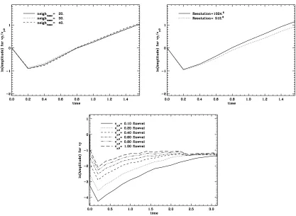
3.3. KHI - NUMERICAL DESCRIPTION 21

Figure 3.2: Left side: Evolution of the linear analytical KHI growth (eq. (3.31)) withν, for equal density layers. Right side: The same, but with DC (eq. (3.30)) assumingν=0.

physical parameters dimensionless in cgs units

Box size 2 2 cm

Mass 4 2780.81 g

velocity 0.387 0.40 km/s

time 1 9.8_·10−6s

Table 3.1: Initial conditions in dimensionless units (first column) and in cgs units (second column). In the text we always refer to dimensionless units.

Analytical growth of the KHI

We briefly analyze the dependence of the linear KHI-growth on the various parameters such as the viscosity (ν) and the density contrast (DC). The parameters are in code units, for conversion to phys-ical units refer to table 3.1.

Fig. 3.2 shows the behavior of[i_·n]withν(left panel) and DC (right panel), important for the com-parison with simulations. The flow-velocity has been set to U =0.387, k=2π (see also 3.3.3). The left panel of Fig. 3.2 assumes equal density layers with the KHI growth determined by eq. (3.31). The right panel shows the variation with DC, where the growth is described through eq. (3.30). In this case we useρ1=1,ν=0, the other parameters are as before. As can be seen in Fig. 3.2, increasing

νand DC suppresses the linear growth and dampens the KHI evolution. We return to this issue in the sections 3.4 and 3.5, when simulating the KHI using different values of DC andν.

Junk, Veronika (2010): Hydrodynamical instabilities and the trace of dark energy within the CMB. Dissertation, LMU München: Fakultät für Physik

HYDRODYNAMICAL

I

NSTABILITIES AND

THE

TRACE OF

DARK

E

NERGY

WITHIN THE

CMB

HYDRODYNAMICAL

I

NSTABILITIES AND

THE

TRACE OF

DARK

E

NERGY

WITHIN THE

CMB

Dissertation

Ph.D. Thesis

Veronika Junk

Vorwort

Contents

List of Figures

List of Tables

Zusammenfassung

Summary

Chapter 1

Motivation

1.1

Part I : Modelling Shear Flows with SPH and Grid Based Methods

1.2

Part II : The Trace of Dark Energy captured within the CMB

Theoretical Basics

2.1

Basics of Hydrodynamics and Instabilities

2.2

Numerical Methods

∑

∑

∑

∑

∑

∑

∑

∑

∑

∑

∑

∑

∑

∑

∑

Chapter 3

Modelling Shear Flows with SPH and

Grid Based Methods

3.1

Introduction

3.2

KHI – analytical description

∑

∑

∑

3.3

KHI - numerical description