1 Modeling the strategies for improved efficacy and crosslink depth of photo-initiated polymerization and phototherapy
Jui-Teng Lin 1, Hsia-Wei Liu 2, Kuo-Ti Chen 3, and Da-Chuan Cheng 4,*
1New Vision Inc., 10F, No. 55, Sect.3, Xinbei Blvd, Xinzhuang, New Taipei City, Taiwan; E-Mail: [email protected]
2Department of Life Science, Fu Jen Catholic University, No. 510, Zhongzheng Rd., Xinzhuang, New Taipei City, Taiwan 24205, E-Mail: [email protected]
3Graduate Institute of Applied Science and Engineering, Fu Jen Catholic
University, Xinzhuang, New Taipei City, Taiwan.
E-mail: [email protected]
4 Department of Biomedical Imaging and Radiological Science, China Medical University, Taichung 404, Taiwan
E-mail: [email protected]
* Author to whom correspondence should be addressed; E-Mail: [email protected] Tel.: +886-4-2205-3366 (ext. 7803); Fax: +886-4-2208-4179.
ABSTRACT: Optimal conditions for maximum efficacy of photoinitiated polymerization are theoretically presented. Analytic formulas are shown for the crosslink time, crosslink depth and efficacy function. The roles of photoinitiator (PI) concentration, diffusion depth and light intensity on the polymerization spatial and temporal profiles, for both uniform and non-uniform cases, are presented. For optimal efficacy, a strategy via controlled PI concentration is proposed, where re-supply of PI in high light intensity may achieve a combined-efficacy similar to low light intensity, but has a much faster procedure. A new criterion of efficacy based on the polymerization (crosslink) [strength] and [depth] is introduced. Experimental data are analyzed for the role of PI concentration and light intensity on the gelation time and efficacy.
Keywords: polymerization modeling; kinetic; photoinitiator; optimal efficacy; crosslinking.
1. Introduction
collagen in aqueous solutions ex vivo, including physical interactions, chemical reactions or photochemical polymerization [2-5]. The advantages and limitations of chemical cross-linking, or so-called “click” chemistry, have been discussed by many researchers [6-12], specially for the thiol-click reactions which include Michael-addition [12] and the thiol-ene reaction [8-11,13,14], where light sources both in UV [6,8] and visible spectra [7,9-12] have been used to initiate polymerization and crosslinking.
The kinetics of photoinitiated polymerization systems (PPS) have been studied by many researchers for uniform photoinitiator distribution or for the over simplified cases that the photolysis product becomes completely transparent after polymerization or constant light intensity [14-17]. Previous models of PPS [18-21] assumed either a constant light intensity [20] (for thin polymers), or a conventional Beer-Lambert law [18, 19, 21] for the light intensity. For more realistic systems, the distribution of the photoinitiator is non-uniform and the UV light may still be absorbed by the photolysis product besides the absorption of the monomer. To improve the efficiency and spatial uniformity (in the depth direction) particularly in a thick system (>1.0 cm), we have presented the numerical results using a focused light [21] and two-beam approach [22] for the case of uniform PI distribution; and analytic and computer modeling for the non-uniform case [23].
Photopolymerization offers two major categories of biomedical applications: (a) photodynamic therapy (PDT) using light-initiated oxygen free radical; and (b) crosslinking (or gelation) of biomaterials using radical-substrate coupling for tissue engineering [1,2]. In general, both type-I and type-II reactions can occur simultaneously, and the ratio between these processes depends on the types and the concentrations of PI, substrate and oxygen, and kinetic rates in the process [24-26]. The kinetics and macroscopic modeling of PPS for anti-cancer have been reported by Zhu et al [24] and Kim et al [25], which, however, are limited to the type-I oxygen-mediated process. Lin reported the kinetic modeling for both type-I and type-II mechanism for the application in corneal collagen crosslinking (CXL) [26,27], where the temporal and spatial profiles of PI concentration and the CXL efficacy were also reported [28]. The treated corneas in CXL has a much smaller thickness (approximately 500 um, or 0.05 cm) than the thick polymer system (approximately 1.0 cm). Therefore, the PPS depth-profile and optimal features in thick polymers require further studies. Accelerated CXL has been clinically used for faster procedure (within 3 to 10 minutes) using higher light intensity of 9 to 45 mW/cm2, in replacing the conventional 3 mW/cm2 which took 30 minutes [27]. However, to our knowledge, no efforts have been done for fast PPS in thick polymers using a high light intensity.
parameters are competing factors, and therefore optimal condition is required for best outcomes. Furthermore, environment conditions such as the internal and external amount of oxygen and PI concentration control are critical in determining the efficacy.
In this study, we will investigate the roles of PI initial concentration and light intensity and fluence (dose) on type-I and type-II efficacy, for both uniform and non-uniform cases. For optimal efficacy, strategy via controlled PI concentration will be presented, for the first time, where re-supply of PI concentration during the PPS is defined by a polymerization (crosslink) time which is inverse proportional to the light intensity [27]. Furthermore, we will define, for the first time, a new concept based on a “volume efficacy” defined by the polymerization (crosslink) strength and depth. Finally, the reported measurements of the role of light intensity [9], the gelation kinetic profiles [13] and the PI concentration [29], will be analyzed by our formulas.
2. Methods and Modeling systems
2.1 Photochemical kinetics
As previously reviewed by Lin [26,27] for CXL, the photochemical kinetics has three pathways which are revised for a more general polymer system and briefly summarized as follows. We will limit the kinetic to the simple case of radical-mediated mechanism, although more complex, two-step thiol–Michael mechanism, involving anionic centers reactive
intermediates may also occur [19,20].
In type-I pathway, the excited PI triple-state (T3) can interact directly with the substrate (A); or with the ground state oxygen (O2) to generate a superoxide anion (O-), which further reacts with oxygen to produce reactive oxygen species (ROS). In comparison, in type-II pathway, T3 interacts with (O2) to form a reactive singlet oxygen (O*). In general, both type-I and type-II reactions can occur simultaneously, and the ratio between these processes depends on the types and the concentrations of PI, substrate and oxygen, the kinetic rates involved in the process [26].
Referring to the kinetic pathways shown by our previous study, Fig. 1 and 5 of Ref. [26], a set of quasi steady-state macroscopic kinetic equations for the time (t) and spatial (z)
profiles of PI ground-state, C(z, t), oxygen molecule [O2], and light intensity, I(z,t), are constructed [26]
dC(z,t)
dt = −b[g + g′]C (1.a)
d[O2]
dt = −sbCG + P(z, t) (1.b)
(1.
dI(z,t)
dz = −A′(z, t)I(z, t) (1.c)
A′(z, t) = 2.3[(a′− b′)C(z, t) + b′C
0(z)] + Q (1.d)
where b=aqI(z,t); a=83.6wa’; w is the light wavelength (in cm); a’ and b’ are the molar
extinction coefficient (in 1/mM/%) of the initiator and the photolysis product, respectively; Q is the absorption coefficient of the monomer and the polymer repeat unit. I(z,t) has a unit of mW/cm2. In Eq. (1.d), we have included the light intensity in the polymer given by a time-dependent, generalized Beer-Lambert law [27]. We have also included in Eq. (1.b) the oxygen source term P (z, t) = p(1-[O2]/[O0]), with a rate constant p to count for the situation when there is an external continuing supply, or nature replenishment (at a rate of p), besides the initial oxygen in the polymer.
Eq. (1.a) defines the type-I process given by, g=k8[A]G0/k3, G0=1/([O2] +k+K’); and type-II
process given by, g’’=K’(C+d) G(z), with G(z)= [O2]G0, k=(k5+k8[A])/k3; K’= k12/ (k6+ k12(C+d) + k72[A]); d is a low concentration correction related to the diffusion of singlet oxygen [14]. [A] is the substrate concentration; q is the triplet state quantum yield given by q=k2/(k1+k2); s=s1+s2, with s1 and s2 are the fraction of [O2] converted to the singlet oxygen and other ROS, respectively, in type-I and type-II [16]. All other rate constants, kj, kij are defined by the reaction paths shown in Fig. 1. Greater details of Eq. (1) can be found in Ref. [14] and [16].
We note that Eq. (1) was also presented by Kim et al [14] for the anti-cancer kinetics.
However, they have assumed a constant light intensity, i.e., A’ (z, t) is a constant in Eq. (1.d).
They also ignored the contribution from the type-I term, g or k8[A], since type-II is dominant in their anti-cancer process. Most of the previous models [18-21] have also ignored the dynamic absorption factor, A (z, t) shown by Eq. (1.d), due to the strong depletion of PI concentration [25]. Greater detail of the kinetics shown by Fig.1 and the complex coupled equations prior to the use of quasi steady-state condition have been discussed in a corneal crosslink model for both type-I and type-II [16], and in thick polymer systems for type-I [25-28]. This article will focus on various strategies for optimal efficacy.
The solution of the light intensity is given by the integration of A’(z,t) of Eq. (c), which, in
general, is time and z dependent due to the depletion of C(z,t). The first-order solution of Eq. (1.a) is given by C(z, t) = C0F(z)exp(-Bt), with B=bg=a’wgI(z), assuming b and g are time -independent. One may also use an averaged A’ (z, t) in Eq. (1.d), which has an initial value A1, (with b’=0) and a steady state value A2 (with C=0), given by: A1=2.3a’C0F’+Q, and
A2=2.3b’C0F’+Q, with F’(z)=1-0.25z/D; the mean value is given by A=0.5(A1+A2). Depletion of C (z, t) will also affect the time-dependent profiles of the intensity, I (z, t), which in general will not follow the conventional Beer-Lambert law (BLL), and should be governed by a generalized, time-dependent BLL, the Lin-law, first presented by Lin [27,28]. Greater detail of
Lin’s law is derived as follows. Using the approximated I(z,t)=I0 (1-Az) in the B-term of exp(-Bt), integration of C(z,t) over z becomes (for the case of F=1), C0 G(z) exp(-aE0), with
G(z)=[exp(B’z) -1]/B’, B’=0.5aE0A, A=0.5(A1+A2). Therefore, the z-integral of A’(z,t) of Eq. (1.d) leads to the light intensity governed by the Lin-law as: I(z,t)=I0 exp[-(A0 + A3(z,t))z], with A0=2.3b’C0 + Q, and the time-dependent component, A3(z,t)= 2.3(a’-b’)C0(1+B’z)exp(-B2t), where we have approximated G(z)= 1+B’z, and B2 = a’wgI0 = B(z=0). Comparing Lin-law and BLL, there are two modifications: the time dependent term A3, and the nonlinear z-dependent term, G(z). Therefore, BLL is the special case of Lin-law when B’= B2 = 0. The Lin-law provide a more accurate analytic formula (comparing to the exact numerical solution) than the
time-average law of A’(z,t), which is independent, where as G(z) of Lin-law includes the z-dependent of C(z,t). Accuracy of Lin-law may be justified by the numerical solutions (to be presented elsewhere).
2.3. Crosslink Time (T*) and Depth (z*)
For a PI initial distribution function given by C0(z)=C0F(z), with F(z)=1-0.5z/D, and D be the distribution depth, the solution of Eq. (1.c) gives I0(z,0)=I0(1-0.25z/D). When D>>1.0 cm, F=1 represents a flat (or uniform) PI distribution. Analytic solution of Eq. (1) is needed to derive the formulas of crosslink time (T*) and depth (z*). For g>>g’, we obtain a first-order solution, C(z, t) = C0F(z)exp(-Bt), with B=bg=a’wgI(z). Using a time-averaged A (z)=0.5(A1+A2). A crosslink (or gelation) time T* may be defined by when the PI concentration C(z, t=T*) = C0 exp(-M), with M = 4, or C(z, t) is depleted to e-4 = 0.018 of its initial value. We obtain an analytic formula T*(z)=T0 exp(Az), where T0 is the surface crosslink time given by T0=M/(B’I0), B’=aqg, which is inversely proportional to the light initial intensity, since b=aqI(z). T* may be also defined by the level of photopolymerization efficacy, or the saturation time (Tc), to be discussed later. Another important parameter is called crosslink (or gelation) depth (z*) defined by a depth having PI concentration C(z,t) reduced to 1/e4 (or 1.8%) of its initial value (at t=T*). Therefore, it is given by (for the case of flat distribution or F=1) z*=(1/A) ln(B’E0/M), with B’=aqg, M=4, which is an increasing function of the light fluence (or dose), E0. In general, for F<1 (with D< 1.0 cm), A is also z-dependent and z* needs numerical calculation.
2.4 Efficacy Profiles
Photopolymerization efficacy is defined by the amount of monomers [M] converted to
polymers initiated by light, Ceff =1-[M]/[M]0 = 1-exp(-S), with S-function for type-I (S1) and
type-II (S2), and the overall efficacy is given by Ceff=1-exp[-(S1+S2)]. Replacing g=k8[A]G0/k3,
by an overall rate constant (K) including all polymerization chain reactions, and using the
first-order solution of C(z,t) and I(z,t) with the time average A(z), the analytic S-function (for
𝑆1= √4𝐾𝐶𝑜𝐹exp (𝐴𝑧)/(𝑎𝑞𝑔𝐼𝑜) 𝐸′ (2.a)
𝐸′ = [1 − exp(−0.5𝐵𝑡)] (2.b)
which is a nonlinear function of the light dose (E0) given by the Taylor expansion of its transient
term E’= 0.5aqgE0(1- 0.5aqgE0+…), S1= [KC0F]0.5(1- 0.5aqgE0+…)t, which does not follow the Bunsen–Roscoe reciprocal law (BRL). In contrast, type-II efficacy, given by the time integral of [IC] follows the BRL [26]. A saturation time (Tc) may be defined by Eq. (3.b) when E1=0.87, or 0.5BTc=2, which gives us Tc=4/B=4/(bg)= [4/(aqgI0)] exp(Az) = T0 exp(Az), with the surface saturation time given by T0=4/(aqgI0) =1000/I0, for aqg=0.004. We note that the saturation time (Tc) equals the crosslink time (T*), when M=4, and it also defines the gelation time, or crossover
time. At t=T*, the transient term of Eq. (3), E’=0.87 and the PI concentration is depleted to 1.8%
of its initial vale.
The S-function for type-II is much more complex than type-I and requires numerical solutions to be shown later. For analytic results for type-II dominant case (with g’>>g), we assume an approximated oxygen concentration given by [O2] = [O0] –m’btC0, with m’ being a fit parameter. Using the first-order solutions of C(z, t) and I(z, t) as type-I, the time integral of Eq. (2.b) leads to (for k<< [O0] and p=0),
S2= (𝑓𝑠𝑎𝑔)Co[(1 − k/[O0])(E′ + 𝑑t) − HO (3)
where HO is a high-order term. Eq. (4) shows that the type-II efficacy is an increasing function of C0 [O0]; and S2has a transient state, E’, proportional to the light dose, E0= I0t; and steady-state is only dose-dependent (for the case of p=0) to be justified numerically later.
2.4 Optimal Efficacy
S1 has maximum value at a crosslink depth (z=z*) given by taking dS1/dz =0. For the case of F=1.0 (or uniform PI concentration, with D>>1.0 cm), it is given by the condition of Bt=1.25, which gives an analytic formula z*=(1/A)ln(E’/1.25), with E’=aqgE0. And the corresponding PI concentration is given by C0*=[ln(E’/1.25)]/z -2.3Q]/[1.13(a’+b’)F]; the maximum S1 is given by
when E’=0.714. For the case of non-uniform PI concentration (with D is 0.5 to 1.0 cm), these optimal conditions require numerical calculations to find the peaks of S1.
2.5 Maximum intensity
2.6 Nonlinear scaling law
As predicted by our S1 formula, the efficacy at transient state (for small dose) is proportional to tI00.5, however, at steady-state, it is a nonlinear increasing function of [C0/I0] 0.5 or [t/E0]0.5. This nonlinear scaling law predicts the clinical data more accurate than the linear theory of Bunsen Roscoe law (BRL) [26]. Accelerated PPS based on BRL, therefore, has undervalued the exposure time (t) for higher intensity using the linear scaling of t = [ E0 /I0], rather than t = [ E0 /I0]0.5, based on our nonlinear law. To achieve the same efficacy, higher PI concentration requires higher light intensity; and for the same dose, higher light intensity requires a longer exposure time.
The BRL is based on the conventional Beer-Lambert law for light intensity without PI depletion, such that I(z) is time-independent, and C(z,t)=constant=C0F, therefore, 𝑆1= √4𝐾𝐶𝑜𝐹𝐸𝑜 exp (𝐴𝑧) which is a linear function of the dose E0 = (tI).
Our nonlinear law, as shown by Eq. (2) predicts that, for the same dose, higher intensity depletes the PI concentration faster and reach a lower steady-state efficacy. Further
discussion will be shown later. As shown by our S-formula, diffusion depth (D) also pays important role. Larger D will achieve higher efficacy as shown by the PI distribution function, F(z)=1-0.5z/D, which is an increasing function of D, and F=1.0 for the flat (uniform)
distribution case. The above features have been clinically shown in corneal crosslinking [26], but not yet for other PPS.
2.7 Volume efficacy
The new concept of a volume efficacy (Ve), first introduced by Lin [30], is defined by the product of the crosslink (or gelation) depth (CD) and local [S-function], or Ve=[1-exp(-S’)], with S’=zS/z0, where z0 is the polymer thickness, and z is the CD defined earlier and given by z=(1/A)ln(B’/E0), with B’=b/M, and E0 is the light dose. We note that the effective S requires a threshold condition, or S>S*, with S*>1.5, such that the local efficacy Eff=1-exp(-S*)>0.87.
Based on our z*-formula, S-formula, Eq. (4), and S profiles shown by Figs. 5 to 9, we
propose a new criterion of PPS efficacy based on the product of [strength] (or S1) and [depth]
(or z*), i.e., the [volume] of polymer being cross-linked. Furthermore, a threshold dose is
required and this threshold limits the maximum light intensity (and a minimum crosslink time)
as discussed earlier. For a given C0, deeper crosslink may be achieved by larger fluence (E0).
However, to achieve uniform and sufficient efficacy by a minimal E0, one requires an optimal
range of D, I0 and C0. An optimal goal is to gain maximum crosslink “volume”, or
[strength]x[depth], as well as polymerization uniformity, specially for thick polymer of 1.0 to
1.5 cm. Greater details are discussed as follows.
Given a threshold S function (S*), the condition for a minimum C0 (C*) is give by S>S*. We
𝐶∗= 𝐼
0G′ exp(−Az) (4.a)
Where S0=[4K/(aqg)]0.5, G’=[S*/(E’S0)]2, which is an increasing function of light intensity, I(z,t),
and S*. This condition is governed by the ratio C*/I0, rather than C* alone, and it is almost
independent to the light dose. A second condition defining the maximum C0 (C’) is given by
the formula with z*> z’, with z’ being the minimum crosslink depth. We found, from the
z*-formula and the average A(z),
𝐶′ = [(Q′/z′) − Q]/[1.15(𝑎′+ 𝑏′)] (4.b)
where Q’=ln[B’E0/M], with B’=aqg. Eq. (4.b) predicts that to achieve a minimum depth (z’),
larger dose is needed for a higher PI concentration. In contrast to C* (which is proportional to
the light intensity), C’ is mainly governed by the light dose. Eq. (4) provides the combined
condition for the range of PI concentration, C*< C0 < C’. Applications of these conditions for
specific polymers will be presented elsewhere.
For type-II mechanism in anti-cancer, the cell viability is given by CV=1-Ve. We should note that both CD and S are increasing functions of the light dose, however, they are competing functions with respect to the PI concentration. Higher C0 offers higher S (or local efficacy) but it has a smaller depth (due to the larger absorption, or larger A-value). The general feature of Ve may be stated as follows: increasing light dose (for a fixed C0) offers both higher [local efficacy] and [depth], and Ve; however, increasing C0 (for a fixed light dose) suffers a shallow depth, although the [local efficacy] increases. Therefore, there is an optimal C0 for maximum Ve. Numerical results and application for cell viability in anti-cancer will be presented elsewhere.
3. Results and Discussions
The Abbreviations, key parameters and formulas of this study are summarized in Table 1.
3.1 Concentration profiles
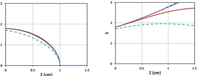
Numerical results of Eq. (1) are shown in Fig. 1 for the PI concentration dynamic profiles.
One may see that depletion of PI starts from the polymer surface, and gradually into the
volume (z>0). We note that the PI concentration profile is an increasing function of z for the
Fig.1 The normalized photoinitiator concentration profiles for uniform (left figure) and non-uniform (right figure, with D=1.0 cm) PI initial distribution, for t=0 (curves 1) and t=50, 100,
150, 200, 300, 350 seconds (curves 2 to 7) with quantum yield q=1.0, a’=0.2(mM·cm)–1, b’=0.15
(mM·cm)–1, and Q=0.1 (1/cm) [23, 27].
3.2 Efficacy profiles
We choose typical values of: a’=0.2(1/mM/cm), b’=0.1(1/mM/cm), Q=0.1 (1/cm), q=0.5,
aqg=0.012 cm2/mW; the mean A(z)=0.35C0F(z)+0.23, B=(0.006I0)exp(-Az)., with C0 in mM, I0 in
mW/cm2. Eq. (2.a) gives a normalized S-function defined by S=S1/S0, where S0=[4K/(aqg)]0.5 is a
proportional constant, such that
𝑆 = 𝐸′√(𝐶𝑜𝐹/𝐼𝑜 )exp (𝐴𝑧) (5)
Based on Eq. (5), we will investigate the roles of C0, I0 and D on the spatial (z) and
temporal (t) profiles of S1, for both uniform and non-uniform cases. In the follow figures, we
show the normalized S-function based on Eq. (5) for S0=4, or K/(aqg)=4. In addition, the
transient factor E’ is based on aqg=0.012, or B=(aqg)I(z)=0.012I(z), and K=4(aqg)=0.048, fit
empirically from the PI concentration profile. [ ].
Fig. 2 shows the time profiles of S versus time (left figure) and versus dose (right figure)
for various light intensity I0= (10,15,20,30) mW/cm2, for D= 1.0 cm, C0=3 mM, at z=0.5 cm. Fig. 3
shows the spatial profiles of S for various exposure time, t= (100,200,300,400) s. Fig. 4 compares
profiles for low and high light intensity at I0= 10 (left figure) and 20 (right figure) mW/cm2, for
the non-uniform case with D=1.0 cm.
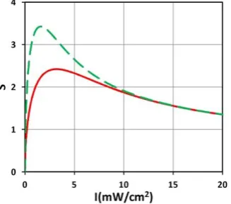
Fig. 5 shows S versus PI concentration (C0), for z=0 and 0.5 cm, for D=1.0 cm, I0=10
mW/cm2. Fig. 6 shows the temporal file of S versus light intensity (I0), for for z=0 and 0.5 cm,
for D=1.0 cm, C0=2 mM, for t=100 s (red curve) and 200 s (green curve).
We note that the transient factor E’ is scaled by (aqg) and the S1 function is scaled by
S0=[4K/(aqg)]0.5. Therefore, the above profiles maybe easily re-produced for a given values of K
(q) or effective kinetic rate constant (K). Therefore, our S-formula, Eq. (5), is a general analytic
equation for NOM type-I photopolymerization including corneal crosslinking and polymer
gelation.
Fig. 2. Time profiles of S versus t (left figure) and versus dose E0 (right figure) for various light
intensity I0= (10,15,20,30) mW/cm2, for D= 1.0 cm, C0=3 mM, at z=0.5 cm, where red-curve is for
the lowest intensity at 10 mW/cm2.
Fig. 3. Spatial profiles of S for various exposure time t = (100,200,300,400) (for curves low to
top), for light intensity I0= 10 (left figure) and 20 (right figure) mW/cm2, and D= 1.0 cm, C0=2
mM.
Fig. 4. Same as Fig. 3, but for D= 0.5 cm (left figure) and D=20 cm (right figure), for light intensity
Fig. 5 Steady-state S versus PI concentration (C0), for z=0 (left figure) and z=0.5 cm (right figure),
for D=1.0 cm, I0=10 mW/cm2.
Fig. 6 Temporal profiles of S versus light intensity (I0), for t=100 s (red curve) and 200 s (green
curve), and z=0.5 cm, D=1.0 cm, C0=2 mM,
3.3 Summary
From the above figures, and Eq. (2), we are able to summarize the important “common”
features for NOM type-I PPS, These common features should cover both thin and thick
polymers, including corneal crosslinking and polymer gelation. Unlike the assumption of a
constant light intensity, which is valid only for very thin polymer, our formulas (including the
PI depletion and dynamic of light intensity) is valid for all polymer thickness.
(i) Fig. 2 (left figure) demonstrates that higher light intensity has a faster rising efficacy, but a
lower steady-state value due to its faster depletion of PI concentration. As also shown by our
formula, Eq. (5), that the efficacy at transient state (for small dose) is proportional to tI00.5.
However, at steady-state (with E1=1), it is a nonlinear function of [C0/I0] 0.5 or [t/E0]0.5. This
nonlinear scaling law predicts the clinical data more accurate than the linear theory of Bunsen
(ii) Fig. 2 (right figure) demonstrates that for the same dose (E0), all light intensity has the same
crosslink time, as shown by Eq. (4.b), E1=1-exp(-Bt), with Bt=bg=aqg (E0) which depends only
on E0, independent to I0.
(iii) As shown by Fig. 3 that higher light intensity has smaller efficacy, reduced by a factor of
1.43 when the intensity is doubled (for the same dose).
(iv) As shown by Fig. 4, small diffusion depth (with D=1.0 cm) has a more uniform but lower S
profile; whereas for large D (or flat, uniform PI concentration) has higher efficacy, but
non-uniform profile.
(vi) As shown by Fig. 5, optimal PI concentration (for maximum S) exits for z>0, but not for z=0.
This optimal feature only exists in thick polymers (with z>0.5 cm), and very high PI
concentration, C0>30 mM. Under normal situation (with C0<10 mM), this optimal value does
not exist.
(vii) Similarly, as shown by Fig. 6, there is an optimal light intensity (for a given time), but not
for light dose (shown by Fig. 2). Moreover, as predicted by Eq. (2), higher intensity has smaller
efficacy (at steady-state, E’=1). To overcome this drawback of high light intensity, a novel
method will be discussed later.
3.4 Analysis of experimental results
The reported measurements of Fairbank et al [9], Lin et al [13], ad O’Brart et al. [29] for
the crossover time, gelation kinetic profile and role of PI concentration are analyzed by our
formulas as follow.
Fig. 3.b of Fairbank et al [8] indicated that the crossover time is a decreasing function of light intensity and the absorption constant (a‘). Our crosslink time formula, on surface (z=0), T0 (in seconds) = 4/(aqgI0)=1000/I0, for aqg=0.004. Therefore, T0=100 s. For I0=10 mW/cm2, and A=0.46 (1/cm), at z=1.0 cm, T*=100 exp(Az) = 158 s, which is comparable to Fig. 3.b of Fairbank for L=0.5 mW/cm3 (for LAP curve). The measured crossover time shows the same trend as our theory that crosslink time is a decreasing function of light intensity. Moreover, Fairbank et al [9] also showed the time required to reach the gel point during the solution polymerization of PEGDA is lower for LAP than for I2959 (at 365 nm) at comparable intensities and initiator concentrations. This may be realized by our formula that Tc is predicted to be inverse proportional to (a’), the molar extinction coefficient, which is 0.218 (1/mM/cm), and 0.04 (1/mM/cm), for LAP and I2959, respectively [9]. Therefore, our formula predicts the S-function of LAP is approximately 5 times of I2959.
Eff=1-exp(-S), is also an increasing function of C0. This feature has been clinically reported by
O’Brart et alin corneal crosslinking [29], where the PI is riboflavin solution initiated by a UVA light at 365 nm. The role of PI concentration on the gelation time, as shown by Fig. 3. of Fairbank et al [8], may be analyzed as follows. Higher PI concentration offers higher crosslink efficacy, therefore less gelation time, although it takes longer time to reach the steady-state.
Above examples demonstrate that our formulas predict very well the measured results,
at last the overall trends. However, the accuracy of our formulas will require accurate
measurement of the parameters involved, such as the rate constant (K), the quantum yield (q),
the molar extinction coefficient of the initiator (a’), the photolysis product (b’), and the
monomer and the polymer repeat unit (Q) et al. In addition, further experimental
measurements should also include the roles of PI concentration and light intensity.
4. Optimal design
The goal of an optimized photo-click hydrogel system is to identify key influencing factors to enable fast gelation (< 2 minutes), minimal photoinitiator-induced toxic response, maximum crosslink depth and uniformity, maximum efficacy, and tunable hydrogel elasticity. This study will focus on these issues which may be well analyzed by our analytic formulas and the numerical-produced figures: (i) crosslink depth and uniformity, (ii) optimized ratio of PI concentration (C0) and light intensity (I0), (iii) improved efficacy.
4.1 crosslink depth and uniformity
Crosslink depth (CD) given by [23, 28] z*=(1/A) ln(B’E0/M), with B’=aqg. For example, when C0 is doubled (from 0.1 mM to 0.2 mM), A increases and z* is reduced by 1.48 times. The z*-formula shows that higher Rf concentration results in an increased (or larger S1) but more superficial (or small z*) cross-linking effect, as also clinically indicated by O’Brart et al
[29]. For a given C0, deeper CD may be achieved by larger light dose (or fluence), E0. However, to achieve clinically acceptable crosslink efficacy by a minimal E0, one requires an optimal range of C0. such that [depth], z*=0.8 to 1.2 cm, and [strength], S1=1.5 to 2.0, or efficacy Eff=1-exp(-S1)=0.78 to 0.86.
As shown by Fig. 4, small diffusion depth (with D=1.0 cm) has a more uniform but lower
S profile; whereas for large D (or flat, uniform PI concentration) has higher efficacy, but
non-uniform profile. Moreover, as shown by Fig. 5, higher PI concentration (with C0=3.0 mM) has
higher by more non-uniform profile, comparing to Fig. 3 (with C0=2.0 mM). Therefore, the
optimal design is to have D=0.4 to 0.6 cm; and C0= 1.5 to 2.5 mM.
As shown by our type-I S-formula, Eq. (2) or (4), higher PI concentration (C0) and lower light intensity (I0) and provides higher efficacy. Higher PI concentration provides higher efficacy, but also suffers more toxicity to the cells. Higher light intensity (I0) may accelerate the crosslink, but has lower efficacy (for the same dose). Therefore, optimal ratio of C0/I0 is required for accelerated and safe crosslink. Furthermore, there is an optimal range for C0 such that the S function larger than a threshed value (S*) for a specified crosslink depth, as defined by Eq. (4) earlier: C* < C0< C’.
4.2 Accelerated Photopolymerization
Another design for optimized photo-click hydrogel system is to identify fast gelation, or an accelerated photopolymerization (APP), based on the Bunsen Roscoe law (BRL) of
reciprocity [27]. This reciprocity-law states that the effect of a photo-biological reaction is proportional only to the total irradiation dose, or fluence, (E=It), or the product of light intensity (I) and exposure time (t). To achieve the same efficacy, the required exposure time based on BRL is given by t=E/I, which gives the protocol for APP. For example, t= (30, 10, 5, 3, 2) minutes for I= (3,9,18,30,45) mW/cm2. The concept of APP has been clinically proven and commercialized in CXL devices for many years [26]. However, there is no reported articles in
more general PPS. Validation of BRL has also been challenged by Lin’s non-linear law and the S-formulas for CXL efficacy [27]. As described earlier that the steady-state efficacy of AP by higher light intensity has the drawback of lower efficacy than lower intensity. To overcome the drawback in AP, a PI concentration-controlled method (CCM) was proposed recently by Lin in corneal crosslinking (CXL) [27], which may be extended for more general PSS as follows.
4.3 Strategy for improved efficacy.
We will discuss two classes of PPS: (a) synthetic polymer sample which is prepared in a
hydrogel form, with PI pre-mixed in the gel uniformly; (b) nature polymer tissue (such as
human cornea or other hydrogels), where the PI solution/drops may be administrated and
diffused from its surface into the volume, having a controllable diffusion depth D.
Class (a) is related to our system with a fixed F(z)=1, and the initial PI concentration
distribution (PICD) can not be controlled by diffusion depth (D), for example, in photoinitiated
polymerization of PEG-diacrylate hydrogel [4]. As shown by Fig. 2 (right figure), the gelation
spatial profile (GSP), for the case of initially uniform PICD (with D>>1.0 cm, or F=1.0), is an
increasing function of the depth (z), i.e., the anterior portion always has less efficacy (gelation).
Strategy using focused light [21] and two-beam illumination [22] were proposed by Lin et al to
For class (b), the PICD profile is controlled by the diffusion time (or the value of D). As
shown by Fig. 4 (left figure) with a non-uniform PICD (with D=0.5 cm), or Fig. 3 (with D=1.0
cm) has a much more uniform crosslinked profile than that of uniform PICD, except that the
center portion (about 0.5 to 1.2 cm) having slightly high efficacy than both ends (near the
surface and the bottom). Comparing Fig. 3 (with C0=2.0 mM) and Fig. 5 (with C0=3.0 mM), we
found that higher C0 has a worse crosslinked profile uniformity. However, low C0 having more
uniformed PSCD, also results a low efficacy (comparing Fig. 3 and 5). Therefore, an optimal C0
should range between 1.5 and 3.0 mM.
Our Formula, Eq. (2) and (5), predict that faster type-I photoinitiated polymerization (gelation or crosslinking) maybe achieved by using a high intensity, which however, also results a low efficacy as shown in Fig. 3. To overcome the drawback of low efficacy in accelerated process using a high intensity, as predicted by our S-formula, a PI concentration-controlled method (CCM) was proposed recently by Lin in corneal crosslinking (CXL) [27]. Greater details based on the crosslink time (T*) and the S-formula, Eq. (4), for a more general PSS, are discussed as follows.
As shown in Fig. 4 that higher light intensity has a faster rising efficacy, but a lower steady-state value due to its faster depletion of PI concentration. Therefore, re-supply of PI drops, (with a supplying frequency defined as Fdrop), during the crosslink would improve the overall efficacy by a combined efficacy given by c-Eff= 1- exp [-(S1 + S2 + S3+.)], where Sj is the individual efficacy for each of the supply of PI. The time to re-supply PI is given by the the crosslink time defined earlier as T*=T0 exp(Az), with the surface crosslink time given by T0= 4/(aqgI0), which is inverse proportional to the light intensity, absorption coefficient (a), quantum yield (q), and the effective kinetic rate constant (g) for type-I pathway.
We note that the Fdrop is proposed by the combined consideration of the crosslink time (T*), which defines when PI is highly depleted (or time needed to reach the steady-state of efficacy); and the surface S-value, which defines the [strength] of crosslink, or the number of re-applying PI drops needed to achieve the same S-value for all intensity ranges (5 to 100 mW/cm2). In Lin’s proposed CCM [27], it predicts the comparable
Fig. 7 Special profile of steady-state combined efficacy with Fdrop=2, for light intensity I0= 30 mW/cm2, C0=2 mM and D= (1.0, 0.5, 0.3) cm, respectively for (S1,S2,S3).
Our S-formula shows that the steady-state S for I0=20 mW/cm2 is 1.43 (or square-root of 2) lower than that of I0=10 mW/cm2, when no re-supply of PI is administered (or Fdrop=0, N=1). Under CCM, for example, in an APP having an intensity 100 mW/cm2, and C0=0.2 mM, we find N=3, and Fdrop= N-1=2, to achieve the same efficacy as the referenced intensity.
When the CCM is used in corneal disease treatment, resupply of riboflavin eye drops was
administrated during the UV light exposure, at every time interval of T*, such that the PI
depletion is continuously supplied by extra drops. For PPS with thick polymer, after the light
exposure for T* period, one needs to turn-off the light and administrated extra PI drops to the
surface of the partially-crosslinked hydrogel, waiting for enough diffusion, then turn-on the
light to finish the crosslinked hydrogel.
Lin proposed CCM for corneal crosslinking (CXL), having a very thin thickness of 0.05 cm (or 500 um) [27]. However, it requires further measurements for general PPS, specially for thick polymers (1.0 to 1.5 cm). While our theoretical predictions provide quantitative guidance or strategy for optimal PPS, their accuracy depends on accurately measured parameters of absorption coefficient, quantum yield, and the effective kinetic rate constant for type-I pathway. Greater detail of CCM for specific polymer systems will be published elsewhere.
5. Conclusion
The overall PPS efficacy is proportional to the light dose (or fluence), the PI initial concentration and their diffusion depths. An optimal goal is to gain fast and maximum
accelerated PPS, which is less efficient than the low intensity (with the same dose) under the normal, non-controlled method.
Acknowledgments
This work was supported by the internal grant of New Vision Inc. KT Chen is partially supported by the Ph.D program of Graduate Institute of Applied Science and Engineering, Fu Jen Catholic University, Taiwan.
Conflicts of Interest
Jui-Teng Lin is the CEO of New Vision Inc.
REFERENCES
1. Fouassier J-P. Photoinitiation, Photo-polymerization, and Photocuring: Fundamentals and Applications. 1995, Hanser Gardner Publications Munich.
2. Chen FM, Shi S. Principles of Tissue Engineering, 4th ed.; 2014, Elsevier: New York, NY, USA.
3. Drury JL, Mooney DJ. Hydrogels for tissue engineering: scaffold design variables and applications. Biomaterials 2003, 24, 4337–4351.
4. Pereira R, Bartolo P. Photopolymerizable hydrogels in regerative medicine and drug delivery. Top. Biomater. 2014, 6–28.
5. Tian Z, Liu W, Li G. The microstructure and stability of collagen hydrogel cross-linked by glutaraldehyde. Polym. Degrad. Stab. 2016, 130, 264–270.
6. Anseth KS, Klok HA. Click chemistry in biomaterials, nanomedicine, and drug delivery. Biomacromolecules, 2016; 17:1–3.
7. Chen MC, Garber L, Smoak M et al. In vitro and in vivo vharacterization of
pentaerythritol triacrylate-co-trimethylolpropane nanocomposite scaffolds as potential bone augments and crafts. Tissu Eng. Part A 2015, 21, 320–331.
8. Chatani S, Gong T, Earle BA, Podgórski M, Bowman CN. Visible-light initiated thiol-Michael addition photopolymerization reactions. ACS Macro Lett. 2014; 3(4):315–318.
9. Fairbanks BD, Schwartz MP, Bowman CN, Anseth KS. Photoinitiated polymerization of PEG-diacrylate with lithium phenyl-2,4,6-trimethylbenzoylphosphinate: Polymerization rate and cytocompatibility. Biomaterials. 2009, 30:6702–6707.
11. Zhang X, Xi W, Wang C, Podgórski M, Bowman CN. Visible-light-initiated thiol-Michael addition polymerizations with Coumarin-based photobase generators: another photoclick reaction strategy. ACS Macro Lett. 2016; 5:229–233.
12. Xi W, Peng H, Aguirre-Soto A, Kloxin CJ, Stansbury JW, Bowman CN. Spatial and temporal control of thiol-Michael addition via photocaged superbase in photopatterning and two-stage polymer network formation. Macromolecules. 2014; 47(18):6159–6165. 13. Shih H, Liu, HY, Lin CC. Improving gelation efficiency and cytocompatibility of visible
light polymerized thiol-norbornene hydrogels via addition of soluble tyrosine. Biomater. Sci. 2017, 5:589–599.
14. Jee E, Bánsági T, Taylor AF, Pojman JA. Temporal control of gelation and
polymerization fronts driven by an autocatalytic enzyme reaction. Angew. Chem., Int. Ed. 2016; 55:2127–2131.
15. Terrones G, Pearlstein AJ. Effects of optical attenuation and consumption of a photobleaching initiator on local initiation rates in photopolymerizations. Macromolecules. 2001, 34: 3195–3204.
16. Kenning NS, Kriks D, El-Maazawi M, Scranton A. Spatial and temporal evolution of the photo initiation rate for thick polymer systems illuminated on both sides. Polym Int. 2005, 54: 1429–1439.
17. Miller GA, Gou L, Narayanan V, Scranton AB. Modeling of photobleaching for the photoinitiation of thick polymerization systems. J Polym Sci Part A Polym Chem 2002;40(6):793–808.
18. Okay O, Bowman CN. Kinetic modeling of thiol-ene reactions with both step and chain growth aspects. Macromol. Theory Simul. 2005; 14:267–277.
19. Reddy SK, Cramer NB, Kalvaitas M, Lee TY, Bowman CN. Mechanistic modelling and network properties of ternary thiol-vinyl photopolymerizations. Aust. J. Chem. 2006; 59(8):586–593.
20. Claudino M, Zhang X, Alim MD et al. Mechanistic kinetic modeling of Thiol–Michael
addition photopolymerizations via photocaged “superbase” generators: An analytical
approach. Macromolecules. 2016; 49(21): 8061–8074. doi:10.1021/acs.macromol.6b01605. 21. Lin JT, Liu HW. Cheng DC. Optimal focusing and scaling law for uniform
photo-polymerization in a thick medium using a focused UV Laser. Polymers. 2014, 6:552-564. doi:10.3390/polym6020552.
22. Lin JT, Liu HW. Cheng DC. Modeling the kinetics of enhanced photo-polymerization under a collimated and a reflecting focused UV laser. Polymers. 2014, 6: 1489-1501. 23. Lin JT, KC Wang. Analytic formulas and numerical simulations for the dynamics of thick
24. Zhu TC, Finlay JC, Zhou X, et al. Macroscopic modeling of the singlet oxygen production during PDT. Proc SPIE. 2007; 6427:6427O81–6427O812.
25. Kim MM, Ghogare AA, Greer A, Zhu TC et al. On the in vivo photochemical rate parameters for PDT reactive oxygen species modeling. Phys. Med. Biol. 2017, 62, R1–
R48.
26. Lin JT. Efficacy S-formula and kinetics of oxygen-mediated (type-II) and non-oxygen-mediated (type-I) corneal cross-linking. Ophthalmology Research. 2018; 8(1): 1-11. 27. Lin JT. A Critical Review on the Kinetics, Efficacy, Safety, Nonlinear Law and Optimal
Protocols of Corneal Cross-linking. J Ophthalmology & Visual Neuroscience, 2018; 3:017. 28. Lin JT, Cheng DC. Modeling the efficacy profiles of UV-light activated corneal collagen
crosslinking. PloS One. 2017;12:e0175002. DOI:10.1371/journal.pone.0175002.
29. O’Brart NAL, O’Brart DPS, Aldahlawi et al, An Investigation of the effects of riboflavin
concentration on the efficacy of corneal cross-Linking using an enzymatic resistance model in porcine corneas. Invest. Ophthalmol Vis Sci. 2018; 59: 1058-1065.
doi:10.1167/iovs.17-22994.
Table 1. Abbreviations and formulas
____________________________________________ PPS: photoinitiated polymerization system BRL: Bunsen–Roscoe reciprocal law BLL: Beer-Lambert law
PI: photoinitiator
Crosslink time (T*) and depth (z*) T*= T0 exp(Az)
T0 (at z=0)= M/(B’I0) z*=(1/A) ln(B’E0/M) Type-I efficacy S-functions:
𝑆1= √4𝐾𝐶𝑜𝐹exp (𝐴𝑧)/(𝑏𝑔𝐼𝑜) 𝐸′ 𝐸′ = [1 − exp(−0.5𝐵𝑡)]
B=B’I(z),B’=aqg.
C0: initial PI concentration (at z=0),
I0 is initial surface (z=0) light intensity; t is exposure time, q : quantum yield of PI triplet state; K is a rate constant; A : average absorption factor, A=0.5(A1+ A2).
________________________________________________
Figure Captions
Fig.1 The normalized photoinitiator concentration profiles for uniform (left figure) and non-uniform (right figure, with D=1.0 cm) PI initial distribution, for t=0 (curves 1) and t=50, 100,
150, 200, 300, 350 seconds (curves 2 to 7) with quantum yield q=1.0, a’=0.2(mM·cm)–1, b’=0.15
(mM·cm)–1, and Q=0.1 (1/cm) [23, 27].
Fig. 2. Time profiles of S versus t (left figure) and versus dose E0 (right figure) for various light
intensity I0= (10,15,20,30) mW/cm2, for D= 1.0 cm, C0=3 mM , at z=0.5 cm, where red-curve is for
lowest intensity at 10 mW/cm2.
Fig. 3. Spatial profiles of S for various exposure time t = (100,200,300,400) (for curves low to
top), for light intensity I0= 10 (left figure) and 20 (right figure) mW/cm2, and D= 1.0 cm, C0=2
mM.
Fig. 4. Same as Fig. 3, but for D= 0.5 cm (left figure) and D=20 cm (right figure), for light intensity
I0= 10 mW/cm2.
Fig. 5 Steady-state S versus PI concentration (C0), for z=0 (left figure) and z=0.5 cm (right figure),
for D=1.0 cm, I0=10 mW/cm2.
Fig. 6 Temporal profiles of S versus light intensity (I0), for t=100 s (red curve) and 200 s (green
curve), and z=0.5 cm, D=1.0 cm, C0=2 mM.