Design And Data Structure of Aco Based Routing Model

(1)

IJEDR1603155

International Journal of Engineering Development and Research (www.ijedr.org)

966

Design And Data Structure of Aco Based Routing

Model

Dr. B. Chandra Mohan Associate Professor VIT University, Vellore

________________________________________________________________________________________________________ Abstract - In the network routing, Ant-Net Routing using Ant Colony Optimization (ACO) technique provides a better result than others due to its real time computation and less control overhead. Comparing to other routing algorithms with ACO it is found that ants are relatively small and can be piggybacked with the data packets. More frequent transmission of ants will not affect the network performance in order to provide updates of routing information for solving link failures. Hence, using ACO for routing in dynamic network seems to be appropriate. Routing in ACO is achieved by transmitting ants rather than routing tables or by flooding LSPs. Even though it is noted that the size of an ant may vary in different systems/implementations, depending on their functions and applications, in general, the size of ants is relatively small, in the order of 6 bytes. This paper explains the design and data structure for effective routing using ACO.

Keywords - Network, Routing, ACO, Swarm Intelligence

________________________________________________________________________________________________________ I. INTRODUCTION

The innovation of ACO techniques starts from the French Entomologist, named Pierre-Paul Grasse. He observed that some species of termites react, which termed as ‘‘significant stimuli’’. The term stigmergy is used to describe the particular type of communication in which the ‘‘workers are stimulated by the performance they have achieved’’. Now the term, stigmergy is used for indirect, non-symbolic form of communication mediated by the environment (Babaei et al, 2015).

This stigmergy is achieved in the ACO using a chemical substance called pheromone, this chemical substance is deposited on the ground when ants walking to and from a food source. Other ants perceive the presence of this pheromone and tend to follow the routes where pheromone concentration is higher (Altiok et al, 2015). Through this mechanism, ants are able to identify and transport food to their nest in a remarkably effective and easy way (Dai et al, 2016).

The real ant and artificial ants are differed in few assumptions, in the real ant behavior the pheromone intensity is reduced over time as the pheromone is the chemical substance and so it evaporates over time (Mulani et al, 2016). However, in the ACO, this can be set to a constant rate, this pheromone evaporation reduces the influence of the pheromones deposited in the early stages of the search (Alshibli et al, 2016), and this property is very useful for adaptive route search in such a situation that frequent path failures.

Comparison of network performance on OSPF and ACO is available in Dorigo et al (2004), Chen et al (2015), and ACO Based Redundant Link Avoidance Algorithm (2011). Detailed study on ACO in various engineering domain is available in Chandramohan et al (2012, 2015).

II.DATA STRUCTURE OF IMPROVED ACO

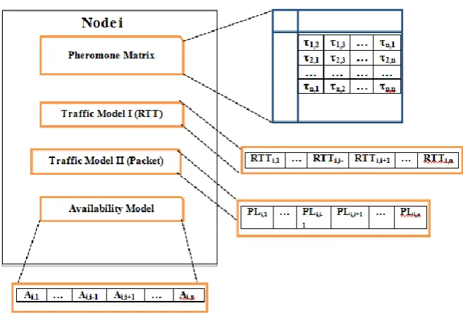
The existing ACO has two data structures, namely, pheromone matrix and traffic model I. The proposed RACO restructures the ACO by introducing two more data structures called traffic model II and availability model. These two data structures are used for identifying congestion free and stable routes. In addition to the extended data structures, the routing decision of proposed RACO is based on a compound probability rule which is the mean probability of existing random probability rule and the two additional probability rule proposed in this work, which is namely probability based on response complexity and probability based on packet loss complexity. In addition to this compound probability rule, the priority model based on availability model is defined for single path routing in the wireless routing.

The data structures of proposed RACO are shown in Figure 1. There are four data structures used in the proposed RACO, namely 1.Pheromone Matrix Model,

2.Traffic Model I, which is used as Round Trip Time (RTT) traffic model, 3.Traffic Model II, which is used as Packet Loss traffic model and 4.Availability Model.

(2)

IJEDR1603155

967

Figure 1. Proposed System Design of RACO

Pheromone matrix of node i is a ‘N x n’ two dimensional matrix, which contains pheromone values of all possible links of the particular node. The rows of the matrix are destination nodes and the columns of the matrix are out-links. And N represents the number of neighbours and n represents the ‘number of nodes -1’. The syntax of the PM is given in the Table 1.

Each value of the pheromone matrix is described as:

τ

i_j_,_d, where,  represents the pheromone deposited on each link from node i to node d through the intermediate node j.

Table 1 Pheromone Matrix of Node i

Out-Link

Destination Link 1

,1

 1,2

… 1,n

2 ,1

 2,2

… 2,n

… … … …

 N,1

 N,2

… N,n

Table 2 Pheromone Matrix of Node 1 of Figure 2 2

,1

 2,3

2,4 2,5 2,6 2,7 2,8

3 ,1

 3,2

3,4 3,5 3,6 3,7 3,8

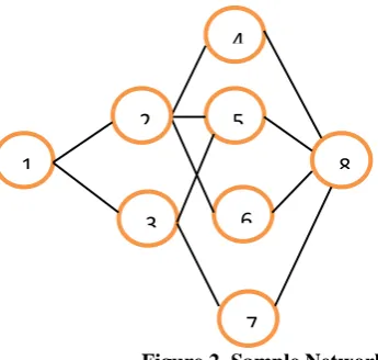
The PMM of node 1 of Figure 2 is shown in the Table 2. In this table, the first column of the PMM is the direct link and the other columns are indirect links. Here number of neighbour nodes of node 1 is two (i.e... node 2 and 3, which is directly connected with node 1). The value of pheromone of unavailable links is assigned as 0, for ex: 3,2 = 0. Initially the pheromone value of each available link is assigned as 1.

(3)

IJEDR1603155

968

Figure 2. Sample Network

The traffic model I is used as Round Trip Time (RTT) Traffic Model. The RTT Traffic model of node i is a one dimensional matrix, in the size of (n-1). The structure of RTTi is given by

RTTi = |RTTi,d|, (1)

where d=1,2,…,n; and d ≠ i.

The traffic model I of each node contains the Round Trip Time (RTT) on all possible links. The syntax of RTT traffic model of each node i is shown in the Table 3 and the RTT traffic model of node 1 shown in the Figure 2 is given in the Table 4.

Table 3 RTT Traffic Model of Node i RT

Ti,1

RT Ti,2

… RT

Ti,i-1

RT Ti,i+1

… RT

Ti,n Table 4 RTT Traffic Model of Node 1 of Figure 2

RT T1,2

RT T1,3

RT T1,4

RT T1,5

RT T1,6

RT T1,7

RT T1,8

The Traffic model II is used as Pocket Loss (PL) Traffic Model. The PL traffic model of node i is a one dimensional matrix, in the size of (n-1). The structure of PL is defined similar to RTT traffic model, PLi is given by equation (2)

PLi = |PLi,d|, (2)

The traffic model II of each node contains the packet loss of all possible links. The syntax of PL traffic model of each node i is shown in Table 5 and the PL traffic model of node 1 shown in the Figure 2 is given in Table 6.

Table 5 PL Traffic Model of Node i

PLi,1 PLi,2 … PLi,i

-1

PLi,i +1

… PLi,n

Table 6 PL Traffic Model of Node 1 of Figure 2 PL1,

2

PL1, 3

PL1, 4

PL1, 5

PL1, 6

PL1, 7

PL1, 8

The Availability model of node i is a one dimensional matrix, in the size of (n-1). The structure of AM is defined similar to RTT and PL traffic model, Ai is given by

Ai = |Ai,d|, (3)

The AM model of each node contains the availability of each node on all possible links. The syntax of AM model of each node i is shown in Table 7 and the AM model of node 1 shown in the Figure 4 is given in Table 8.

Table 7 AM Model of Node i

Ai,1 Ai,2 … Ai,i-1 Ai,i+

1

… Ai,n

Table 8 AM Model of Node 1 of Figure 2

A1,2 A1,3 A1,4 A1,5 A1,6 A1,7 A1,8

III.ROUTE DISCOVERY AND ROUTE MAINTENANCE IN RACO

At regular intervals, ∆t, from every network node S, forward ant, ‘Fs→d’ is launched toward a destination node d to discover a feasible, low-cost path to that node and to investigate the load status of the network along the path. The FA shares the same queues as data packets, so that they experience the same traffic load. Destinations are locally selected according to the data traffic patterns generated by the local workload.

If fsd is a measure in bits or in the number of packets of the data flow from the source S to the destination d (s → d), then the probability of creating a FA is

4

5

6

7

8

1

2

(4)

IJEDR1603155

969 



_n 1 i si sd

f

p

(4)

Ants adapt their exploration activity in this way to the varying data traffic distribution. While travelling towards their destination nodes, the FA keep memory of their paths and of the traffic conditions found. The identifier of every visited node i and the time elapsed since the launching time to arrive at this ith_{node are stored in a memory stack S}

s→d(i). Further the ant builds a path by performing the following steps:

Step 1 (Distribution of Forward Ant)

At each source node i, each FA headed toward the destination node d by selecting the intermediate node j, choosing among its neighbour which is not visited already. The neighbours j is selected with a probability Pijd computed as the normalised sum of the pheromone ijd with a heuristic value ij taking into account the state (the length) of the jth link queue of the current node I is

)

1 N

(

α

1 η

α

τ

p

i ij ijd

ijd

_

_







(5)

The heuristic value ij is a normalised value function (0, 1) of the length of the queue ‘qij’ between the node i and its neighbour j is

il N

1 l

ij ij

q

1 η









(6)

The value of α determines the importance of the heuristic value with respect to the pheromone values stored in the pheromone matrix (). The value ij reflects the instantaneous state of the node’s queues and assuming that the queue’s consuming process is almost stationary or slowly varying, ij gives a quantitative measure associated with the queue waiting time. The pheromone values, on the other hand, are the outcome of a continual learning process. This learning process will register both the current and the past status of the whole network. The two components of the ant decision system,  and , used for the decision system will act both the combination of long-term learning process and an instantaneous heuristic prediction.

Step 2 (Avoid Cyclic Routing)

If an ant returns to an already visited node, the cycle’s nodes are remove and all the memory about them are deleted. This process helps the system to avoid the count-to-infinity problems.

Step 3 (Generate Backward Ant) Condition 1 – Generate BA and delete FA

When the destination node d is reached, the FA Fs→d generates another ant called the backward ant Bd→s and transferred the information stored in the memory of FA then the FA is to be deleted.

Condition 2 – Delete FA on lifetime Basis

The FA is deleted if its life time becomes greater than a value of max_life before it reaches the destination node, which is similar to TTL (Time to Live) in the TCP.

Step 4 (Flow of BA):

The flow of FA and BA have some distinctions. The BA takes the same path as the concern FA travelled, but in the opposite direction. The FA share the same link queues as data packets, but the BA do not share the same link queues as data packets, instead BA uses the higher-priority queues reserved for routing packets. Because the task of BA is to quickly propagate to the pheromone matrices.

IV.RESULTS AND PERFORMANCE ANALYSIS

(5)

IJEDR1603155

970

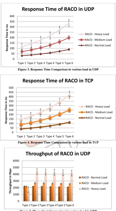
Figure 3. Response Time Comparison in various load in UDP

Figure 4. Response Time Comparison in various load in TCP

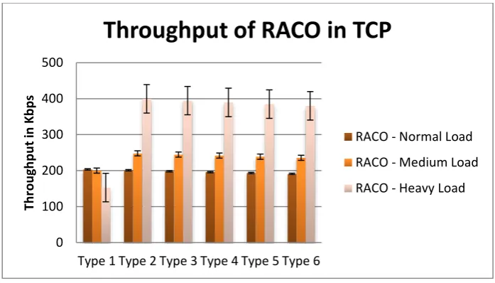
Figure 5. Throughput Comparison in various load in UDP

0 50 100 150 200 250 300 350 400

Type 1 Type 2 Type 3 Type 4 Type 5 Type 6

R

e

sp

o

n

se

Ti

m

e

in

m

s

Response Time of RACO in UDP

RACO - Heavy Load

RACO - Medium Load

RACO - Normal Load

0 50 100 150 200 250 300 350 400 450 500

R

e

sp

o

n

se

Ti

m

e

in

m

s

Response Time of RACO in TCP

RACO - Heavy Load

RACO - Medium Load

RACO - Normal Load

0 1000 2000 3000 4000 5000 6000

Th

ro

u

gh

p

u

t

in

Kb

p

s

Throughput of RACO in UDP

RACO - Normal Load

RACO - Medium Load

(6)

IJEDR1603155

971

Figure 6. Response Time Comparison in various load in TCP

V.REFERENCES

[1] Alshibli, M., El Sayed, A., Kongar, E., Sobh, T.M., Gupta, S.M (2016). Disassembly Sequencing Using Tabu Search. Journal of Intelligent and Robotic Systems: Theory and Applications, 82 (1), 69-79

[2] Altiok, M., Kocer, B (2015). The Analysis of GR202 and Berlin 52 Datasets by Ant Colony Algorithm. International Conference on Advanced Computer Science Applications and Technologies, 103-108

[3] Babaei, N., Tabesh, M., Nazif, S (2015). Optimum reliable operation of water distribution networks by minimising energy cost and chlorine dosage. Water SA, 41(1), 149-156

[4] Chandra Mohan, B. and Baskaran, R (2011). Reliable Barrier-free Services in Next Generation Networks. International Conference on Advances in Power Electronics and Instrumentation Engineering, Communications in Computer and Information Science, Springer-Verlag Berlin Heidelberg, 148, 79-82

[5] Chandra Mohan, B. and Baskaran, R (2012). A Survey: Ant Colony Optimization based recent research in various engineering domains. Expert System with Application, Elsevier, 39(4), 4618-4627

[6] Chandra Mohan, B (2015). Restructured Ant Colony Optimization routing protocol for next generation network, International Journal of Computer Communication and Control, Agora University Press, 10(4), 493-500

[7] Chen, Y., Jia, Y (2015). Research on traveling salesman problem based on the ant colony optimization algorithm and genetic algorithm. Open Automation and Control Systems Journal, 7 (1), 1329-1334

[8] Dai, Y., Zhao, M (2016). Manipulator path-planning avoiding obstacle based on screw theory and ant colony algorithm. Journal of Computational and Theoretical Nanoscience, 13 (1), 922-927

[9] Dorigo, M. and Stutzle, T. “Ant Colony Optimization”, MIT Press, Cambrige MA, 2004

[10] Mulani, M., Desai, V.L (2016). Computational performance analysis of Ant Colony Optimization algorithms for Travelling Sales Person problem. Advances in Intelligent Systems and Computing, 408, 561-569

0 100 200 300 400 500

Th

ro

u

gh

p

u

t

in

Kb

p

s

Throughput of RACO in TCP

RACO - Normal Load

RACO - Medium Load