Article
Multi-Task
Learning
for
Multi-Dimensional
Regression:
Application
to
Luminescence
Sensing
UmbertoMichelucci1,FrancescaVenturini1,2
1
2
3
4
5
6
7
8
9
10
11
12
13
14
15
16
17
18
19
1 TOELTLLC;[email protected]
2 ZürichUniversityofAppliedScience;[email protected]
* Correspondence:[email protected]
Abstract: Theclassicalapproachtonon-linearregressioninphysics,istotakeamathematicalmodel describingthefunctionaldependenceofthedependentvariablefromasetofindependentvariables, andthen,usingnon-linearfittingalgorithms,extracttheparametersusedinthemodeling.Particularly challengingarerealsystems,characterizedbyseveraladditionalinfluencingfactorsrelatedtospecific components,likeelectronicsoropticalparts.Insuchcases,tomakethemodelreproducethedata, empiricallydeterminedtermsarebuilt-inthemodelstocompensatefortheimpossibilityofmodeling thingsthat are, by construction,impossible to model. A newapproachto solve thisissue isto useneuralnetworks, particularlyfeed-forwardarchitectureswithasufficientnumber ofhidden layersandanappropriatenumberofoutputneurons,eachresponsibleforpredictingthedesired variables. Unfortunately,feed-forwardneuralnetworks(FFNNs)usuallyperformlessefficiently whenappliedtomulti-dimensionalregressionproblems,thatiswhentheyarerequiredtopredict simultaneouslymultiplevariablesthatdependfromtheinputdatasetinfundamentallydifferent ways. To address thisproblem, weproposemulti-task learning(MTL) architectures. Theseare characterizedby multiple branches of task-specificlayers, whichhave asinput the output of a commonsetoflayers.Todemonstratethepowerofthisapproachformulti-dimensionalregression, themethodisappliedtoluminescencesensing.HeretheMTLarchitectureallowspredictingmultiple parameters,theoxygenconcentrationandthetemperature,fromasinglesetofmeasurements.
Keywords: multi-tasklearning;non-linearregression;neuralnetworks;luminescence;luminescence quenching;oxygensensing;phasefluorimetry; temperaturesensing
20
1. Introduction
21
The classical use of regression in physics, sometimes also referred to as non-linear fitting, is to try
22
to determinedquantitiesy∈Rdfrom a set ofnmeasurementsx∈Rqwithq∈N, using a theoretical
23
mathematical modely= f(x,w)that depends on a certain numberpof parametersw∈Rp. Typically
24
this is achieved by choosing the parameterswto minimize a selected error function, like the mean
25
square error (MSE), with specific algorithms. To find the best solution forf is a classical optimization
26
problem [1–3]. This method, however, fails to deliver stable and accurate results, for example, when the
27
quantitiesyiwithi=1, ...,dhave different physical meanings and, consequently, depend on different
28
components of the parameter vectorwin fundamentally distinct ways. As a result, the mathematical
29
model may be an insufficient approximation, may be too complex for a stable implementation or may
30
be simply unknown [3].
31
An example where the usual multi-dimensional regression approach fails is in the determination
32
of a substance from changes in its luminescence when several environmental conditions vary in
33
an unknown and uncontrolled way. Luminescence quenching for oxygen detection represents a
34
widespread application relevant in many fields like biomedical imaging, environmental monitoring,
35
or process control [4] (see Section4for details). In this application, the quantity of interest is the
36
concentration of molecular oxygen[O2]. The measured quantity, either the luminescence intensity or
37
luminescence intensity decay time of a special molecule (luminophore), is however equally strongly
38
dependent on the concentration[O2]and the temperatureT. As a result, it is not possible to extract
39
two different physical quantities, namely [O2] and T, from the same set of data. Usually, T is
40
measured separately with another device and given as an input to a mathematical model describing
41
the dependency of those two quantities from the input data. The complexity increases further if more
42
than on luminophore is present, and several parameters (e.g.[O2],[CO2],pH) have to be determined
43
[5–9].
44
A possible method, which recently attracted great interest, is the use of feed-forward neural
45
network (FFNN) architectures, with a certain number of hidden layers and an appropriate number of
46
output neurons, each responsible for predicting the desired variablesyiwithi=1, ...,d. In the example
47
of oxygen sensing, the output layer would have a neuron for the oxygen concentration[O2]and one
48
for the temperatureT. This work shows that, since the output neurons must use the same features (the
49
output of the last hidden layer) for all variables [10,11], FFNNs result insufficiently flexible. For the
50
cases when the variables depend in fundamentally different ways from the inputs this approach will
51
give a result that is at best acceptable, and at worst unusable.
52
This work proposes a new approach, which is based on multi-task learning (MTL) neural networks
53
architectures. This type of architectures are characterized by multiple branches of layers, that get
54
their input from a common set of layers. These type of networks can improve the model prediction
55
performance by jointly learning correlated tasks [10–14]. In particular, the proposed MTL architectures
56
are applied to the problem of luminescence quenching for oxygen sensing. Their performance in the
57
prediction of oxygen concentration and temperature is analyzed and compared to that of a classical
58
feed-forward neural network.
59
In general, the proposed MTL approach may be of particular relevance in all those cases, where
60
the mathematical modely= f(x,w)is not known, too complex or not really of interest and the only
61
goal of the regression problem is to build a system that is able to determineyas accurately as possible.
62
The paper is organized as follows: Section2describes non-linear regression and MTL with neural
63
networks. Section3describes the implementation of MTL and the different neural network studied in
64
this work. Section4reviews luminescence quenching for oxygen sensing. The results are discussed in
65
Section5.
66
2. Theoretical Background
67
This section briefly reviews the theoretical justification for non-linear regression with neural
68
networks, as well as the multi-task learning approach implemented in this work.
69
2.1. Neural Networks for Non-Linear Regression Problems
70
In general, a neural network model is always composed of three parts [15]:
71
• network architecture (number of layers, activation functions, etc.),
72
• cost function,
73
• optimizer (a method or algorithm used to minimize the cost function).
74
when solving classification problems [15]. For regression problems, as the one studied in this work, the most common cost function is the mean square error (MSE), which is defined as
MSE= 1
n n
∑
j=1
d
∑
k=1
(y[kj]−yˆ[kj])2 (1)
wherenis the number of observations in input dataset;y[j] ∈Rdis the measured value of the desired
75
quantity for thejthobservation (indicated as a superscript between square brackets), withj=1, ...,n;
76
ˆ
y[j] ∈Rdis the output of the network, when evaluated on thejthobservation. The optimizer affects
77
the learning performance of the network but does not determine the type of problems the network can
78
solve and therefore will not be discussed here.
79
A regression problem consists in minimizing the cost function, in this case the MSE (Equation
80
1), with respect to the learnable parameters of the network, which are defined in the architecture.
81
The implicit assumption done is that there is an underlying albeit unknown functiongthat describes
82
the relationship between they[j] and the input observations (the measurementsx[j]). Assuming 83
its existence, the neural networks try to approximateg, by composing a big number of non-linear
84
functions. This approach relies on the implicit assumption that a network can approximate any
85
function, whatevergis. For FFNN this assumption is legitimate since it was proved mathematically
86
[16–23]. This mathematical proof thus justifies the use of neural networks for regression problems.
87
Unfortunately, not being a constructive proof, it provides neither the number of layers nor the number
88
of neurons per layer needed to approximateg. It just tells that, with enough neurons, a neural network
89
is able to approximate any function.
90
2.2. Multi-Task Learning
91
Multi-task learning is a machine learning techniques in whichnT learning tasks are solved at
92
the same time, using commonalities and differences across tasks. This approach typically results in
93
improved learning efficiency and prediction accuracy [12–14,24].
94
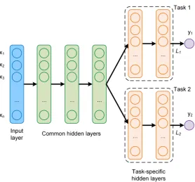
An example of a simple MTL network architecture, which reflects the architectures later used in
95
the paper, is shown in Figure1. This network consists of a series of common hidden layers, followed
96
by two branches (nT =2) each consisting of several task-specific hidden layers.
97
The layers marked in Figure1as "common hidden layers" generate an output, that is typically
98
called a "shared representation". The name comes from the fact that the output of those layers is used
99
to evaluate bothy1andy2. The shared representation is then the input of a set of "task-specific hidden
100
layers", that learn how to predicty1andy2better. Note how the common hidden layers are shared
101
with both the tasks of predictingy1andy2, while the task-specific hidden layers are specific to each
102
task separately. The MTL network of Figure1uses the common hidden layers to find common features
103
beneficial to each of the two tasks. During the training phase, learning to predicty1will influence the
104
common hidden layers and therefore, the prediction ofy2, and vice-versa. A set of task-specific hidden
105
layers will then learn specific features to each output and therefore improve the prediction accuracy.
106
The implicit assumption here is that the tasks have something in common; otherwise this approach
107
will not produce the desired result.
108
Multiple cost functionsLiwithi=1, ...,nT, withnTthe number of tasks, are required to use this network architecture. In the training phase a global cost functionL, defined as a linear combination of the task-specific cost functions with weightsαiwill be minimized
L=
nT
∑
i=1
Figure 1.Example of a MTL network architecture with two tasks and two outputs.
The parametersαihave to be determined during the hyper-parameter tuning phase to optimize the network predictions. In this paper, being the cost function the MSE (Equation1), the global cost function of Equation2is
L=
nT
∑
i=1 αi
1 n
n
∑
j=1
d
∑
k=1
(y[kj]−yˆ[kj])2 (3)
wherenTis the number of tasks;nis the number of observations in input dataset;y[j] ∈ Rdis the
109
measured value of the desired quantity for observationj, withj=1, ...,n; ˆy[j] ∈
Rdis the output of the
110
network, when evaluated on thejthobservation.
111
3. Neural Network Architectures and Implementation
112
In this paper three architectures, one classical FFNN and two MTL, were investigated and
113
compared in the simultaneous prediction of oxygen concentration and temperature. To make the
114
comparison meaningful, the parameters, which are not architecture-specific, were not varied. The
115
details of the architectures are described in the next subsections.
116
In the three architectures investigated the sigmoid activation functions was used for all the neurons
σ(z) = 1
1+e−z. (4)
All the results were obtained with a training of 4000 epochs. The target variablesywere normalized to
117
vary between 0 and 1. Thus, the sigmoid activation function was used also for the output neurons
118
y1andy2. The input measurement, as will be explained in detail in Section4, is a vector inRqwith
119
q=16.
120
To minimize the cost function, the optimizer Adaptive Moment Estimation (Adam) [15,25] was
121
used. The training was performed with a starting learning rate of 10−3 and using batch-learning,
122
which means that the weights were updated only after the entire training dataset has been fed to the
123
network. Batch-learning was chosen because of its stability and speed since it reduces the training
124
time of a few orders of magnitude in comparison to, for example, stochastic gradient descent [15].
Therefore it makes experimenting with different networks a feasible endeavor. The implementation
126
was performed using the TensorFlowTMlibrary.
127
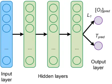
3.1. Network A
128
The first type of neural network investigated has a classical feed-forward architecture, consisting
129
of an input layer, three hidden layers, and an output layer with two neurons[O2]predandTpred. This
130
architecture, labeled here as Network A, is schematically shown in Figure2. The number of neurons of
131
each hidden layerni=nˆis the same. Each neuron in each layer gets as input the output of all neurons
Figure 2.Architecture of the feed-forward network A.
132
in the previous layer, and feeds its output to each neuron in the subsequent layer. The number of
133
neurons was chosen to be ˆn=10, 30, 50, 80. Note that an extensive hyper-parameter search to optimize
134
the network A performance was not performed here since this was not the goal of the paper.
135
3.2. Network B
136
The first MTL network studied is depicted in Figure3. It consists of three common hidden layers
137
with 50 neurons each, followed by two branches, one with two additional task-specific hidden layers
138
used to predict[O2], and one branch without hidden layers used to predict both[O2]andTat the same
139
time. The number of neurons of each task-specific hidden layer is 5. The idea behind this network is to
140
have a system that learns to predict[O2]well, thanks to the further task-specific layers. The predicted
141
T is not expected to be exceptionally good since the common hidden layers must learn to predict
142
[O2]predandTpredat the same time. This architecture can be of applied when one of the outputsyi, here
143
[O2], needs to be predicted with higher accuracy than the other ones. For this network, the global cost
144
function weights used wereα1=0.3 andα2=5.
145
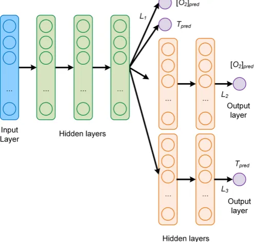
3.3. Network C
146
The last MTL network, depicted in Figure4, consists again of three common hidden layers with
147
50 neurons each, followed by three branches, two with each two additional task-specific layers to
148
predict respectively[O2]andT, and then one without additional layers to predict[O2]andTat the
149
same time. The number of neurons of each task-specific hidden layer is 5, as in the network B. The
150
global cost function weights used wereα1=0.3,α2=5 andα3=1.
151
Figure 4.Architecture of the feed-forward MTL network C.
This network is of interest because of the additional task-specific layers, which are expected to
152
improve the ability of predicting the temperature compared to the network B.
153
3.4. Metrics
154
The metric used to compare results from different network models is the absolute error (AE) for a given observationj, defined as the absolute value of the difference between the predicted and the expected value. For the oxygen concentration[O2][j]theAEis
AE[[Oj]
2]=|[O2]
[j]
pred−[O2]
[j]
meas|. (5)
The further quantity used to analyze the performance of the network is the mean absolute error (MAE), defined as the average of the absolute value of the difference between the predicted and the expected oxygen concentration or temperature. For example, for the oxygen prediction using the training datasetStrain,MAE[O2]is defined as
MAE[O2](Strain) = 1
|Strain|j∈
∑
S train|[O2][predj] −[O2][realj] | (6)
where|Strain|is the size (or cardinality) of the training dataset. For example, in this work|Strain|=20000.
155
TheAETandMAETare similarly defined.
4. Luminescence Quenching for Oxygen and Temperature Sensing
157
To demonstrate its advantages, the MTL approach was applied to the simultaneous determination
158
of the oxygen concentration and temperature of a medium. There are different optical methods used to
159
determine oxygen concentration since this is of great relevance for numerous research and application
160
fields, ranging from biomedical imaging, packaging, environmental monitoring, process control, and
161
chemical industry, to mention only a few [26]. Among the optical methods, a well-known approach is
162
based on luminescence quenching [27–29].
163
The measuring principle is based on the quenching of the luminescence of a specific molecule
164
(luminophore) by oxygen molecules. Because of the collisions of the luminophore with oxygen, both the
165
luminescence intensity and decay time are reduced. Sensors based on this principle rely on approximate
166
empirical models to parametrize the dependence of the sensing quantity (e.g., luminescence intensity
167
or intensity decay time) on influencing factors. The most relevant parameter, which can be a major
168
source of error in sensors based on luminescence sensing, is the temperature of the luminophore, since
169
both the luminescence and the quenching phenomena are strongly dependent on temperature [26].
170
The conventional approach consists in relating the change of the luminescence decay time from the oxygen concentration through a multi-parametric model, called Stern–Volmer equation [28]. The value of the device-specific constants is then determined through calibration. Without going into the details of the analytical model, the measured quantity, the phase shiftθ, is most frequently related to
the oxygen concentration[O2]and temperatureTthrough the approximate equation [30]
tanθ(ω,T,[O2])
tanθ0(ω,T) =
f(ω,T)
1+KSV1(ω,T)·[O2]
+ 1−f(ω,T)
1+KSV2(ω,T)·[O2]
−1
(7)
whereθ0andθ, respectively, are the phase shifts in the absence and presence of oxygen,f and 1− f
indicate the fraction of the total emission of two components under unquenched conditions,KSV1
andKSV2 are associated (Stern–Volmer) constants for each component. Since the phenomena of
luminescence and luminescence quenching are strongly influenced by the temperature, the parameters
θ0,KSV1,KSV2, and f need to be modelled through different temperature dependencies [30]. The
value of the parametrisation quantities is determined through non-linear regression.ωis the angular
frequency of the modulation of the excitation light. Finally, Eq. (7) must be inverted to obtain[O2]as a
function ofθ, T, andω. To be able to have more information as input to our network, we will not use a
singleωfrequency value, but 16. Let’s define
r(ω,T,[O2])≡ tan
θ(ω,T,[O2])
tanθ(ω,T,[O2] =0)
. (8)
The goal of the network is to predict the oxygen concentration and temperature from an array of
171
values of r(ω,T,[O2]) evaluated at a discrete set of sixteen ωi, with i = 1, ...16, that have been
172
used for the measurements. The jth measurement can be written as x[j] = (r[1j],r[2j], ...,r[16j]) with
173
r[ij] = r(ωi,T[j],[O2][j])andi = 1, ...16. Each measurement jcorresponds to a specific tuple of the
174
oxygen concentration and temperature(T[j],[O
2][j]).
175
Summarizing, the conventional approach relies on the measurement of the temperature, which is
176
then used to correct the parameters of the analytical model used to calculate the oxygen concentration
177
[O2]from the measured quantity, the phase shiftθof Equation7. The inadequate determination of the 178
luminophore temperature is one of the major sources of error in an optical oxygen sensor.
179
The neural network proposed in this work defies the difficulties described above by
180
simultaneously predicting both the oxygen concentration and the temperature using 16 values of
181
4.1. Data Generation
183
To have a large enough dataset to train and test the neural networks, synthetic data were used.
184
The model described by Equation (7) was chosen to create the data, being as simple as possible but
185
still capable to describe experimental observations. The values of the parameters for the synthetic data
186
were determined from measurement performed under varying oxygen concentration and temperature
187
conditions. For details on the samples and setup used for the determination of all the parameters the
188
reader is referred to [30].
189
The synthetic data consist of a setSof m = 25000 observations using oxygen concentration
190
values uniformly distributed between 0 % air and 100 % air and five temperatures 5, 15, 25, 35 and
191
45◦C. Please note that in the following, the concentration of oxygen is be given in % of the oxygen
192
concentration of dry air and indicated with % air. This means that 100 % air corresponds to 20 % vol
193
O2. Themdata were split randomly in a training dataset containing 80 % of the data (|Strain|=20000),
194
used to train the network, and a development dataset containing 20 % of the data (|Stest|=5000), used
195
to test the generalisation efficiency of the network when applied to unseen data.
196
Typically when training neural network models, it is important to check if we are in a so-called
197
overfitting regime. The essence of overfitting is to have unknowingly extracted some of the residual
198
variation (i.e., the noise or errors) as if that variation represented an underlying model structure [31].
199
In the case discussed in this work, with increasing network complexity, the network will never go into
200
such a regime since the development dataset is a perfect representation of the training dataset. This
201
leads to almost identical metric values for theMAEfor bothStrainandSdev, regardless of the network
202
architecture effective complexity. This is what we observed while checking the metrics on the two
203
different datasetStrainandSdev. This becomes relevant when dealing with real measurements and not
204
synthetic data.
205
5. Results and Discussion
206
As described in Section4, the applied problem investigated in this work is a complex one since
207
the two quantities to be extracted from the data ([O2]andT) depend from the input in different ways.
208
It is therefore not obvious that is possible to build a model which is able to predict both[O2]andTat
209
the same time with good accuracy.
210
The fist network investigated is the simple FFNN A described in Section3.1. For this network,
211
the number of neurons was progressively increased ( ˆn=10, 30, 50, 80) to study howAE[O2]andAET
212
are affected by an increasingly complex network and to determine if it is possible to obtain a good
213
prediction. The calculatedAE[O2]for differentO2concentrations were grouped in bins of 10 % air for a
214
clearer illustration and are shown in Figure5as a box plot, where the median is visible as a red line.
215
[0,10] [10,20] [20,30] [30,40] [40,50] [50,60] [60,70] [70,80] [80,90]
[90,100]
[O2] ranges (% air)
0 5 10 15 20
Absolu e Error (% air)
Ne work A ( ̂n ̂ 30)
[0,10] [10,20] [20,30] [30,40] [40,50] [50,60] [60,70] [70,80] [80,90]
[90,100]
[O2] ranges (% air)
0 5 10 15 20
Ne work A ( ̂n ̂ 50)
[0,10] [10,20] [20,30] [30,40] [40,50] [50,60] [60,70] [70,80] [80,90]
[90,100]
[O2] ranges (% air)
0 5 10 15 20
Ne work A ( ̂n ̂ 38)
Figure 5.Absolute errorAE[O2]in the prediction of theO2concentration for the different concentration
As it can be seen in Figure5, the results are quite poor if ˆn=30 (results for ˆn=10 are even worse
216
and will not be discussed here). AE[O2]can assume values as big as 18 % air, with a broad distribution.
217
Increasing the number of neurons in the hidden layers to ˆn=50 improves the prediction, reducing
218
both the median and the distribution. A further increase to ˆn=80, however, does not result in better a
219
prediction, showing the limits of this architecture to capture the details of the physical system.
220
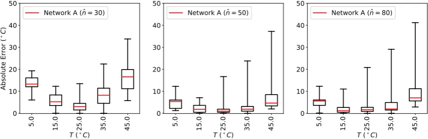
The results for the prediction of the temperature for the same three networks are shown in Figure
221
6. AlsoAETimproves initially by increasing the number of neurons to ˆn=50, but does not get any
222
better when the number of neurons is further increased to ˆn=80. The boxplots of Figure5and Figure
223
6show thatAE[O2]andAETcan assume quite high values, therefore demonstrating how the model is
224
not really able to make a prediction with an accuracy that may be used in any commercial application.
225
5.0 15.0 25.0 35.0 45.0
T (∘C)
0 10 20 30 40 50
Absolute∘Error∘(
∘C
)
Network∘A∘( ̂n = 30)
5.0 15.0 25.0 35.0 45.0
T (∘C)
0 10 20 30 40 50
Network∘A∘( ̂n = 50)
5.0 15.0 25.0 35.0 45.0
T (∘C)
0 10 20 30 40 50
Network∘A∘( ̂n = ̂0)
Figure 6.Absolute errorAETin the prediction ofTfor the different temperatures using network A.
Left: 30 neurons per hidden layer; middle: 50 neurons per hidden layer, right: 80 neurons per hidden layer.
The performance of the three FFNN of type A can be summarized calculating theMAEas defined
226
in Equation6. The results are listed in Table1. Consistently with what previously observed for the
227
absolute error, the best network performance is obtained with ˆn=50, achieving a mean absolute error
228
ofMAE[O2]=1.7 % air andMAET=1.7 ◦C.
229
Table 1. Summary of the performance for the FFNNs A
ˆ
n MAE[O2] MAE[T]
30 6.0 % air 9.3◦C
50 1.7 % air 1.7◦C
80 2.3 % air 2.3◦C
For a practical application, the probability density distribution of theAEs for both parameters
230
represent a much fundamental quantity since it carries information on the probability of the network
231
to predict the expected value. For this reason, the kernel density estimate (KDE) of the distributions of
232
theAEs was analyzed. The results forAE[O2]andAETfor the three variations of FFNN A are shown
233
in Figure7and8, respectively.
234
From Figure7and8can clearly be seen that increasing the number of neurons helps at the
235
beginning. A further increase in ˆndoes not produce an improvement in prediction quality, on the
236
contrary it gets worse. These results indicate that this simple FFNN can extract at the same time the
237
two quantities with an accuracy which is at best poor and at worst unusable.
238
Networks B and C try to address this problem by adding, as described in previous sections,
239
respectively one and two branches after the last hidden layer in network A. The results of the prediction
240
from the networks B and C are then compared to those from network A with ˆn=50. Figure9shows
241
the calculatedAE[O2]for the three networks for the same[O2]intervals as before as a box plot, where
242
the median is visible as a red line.
0 5 10 15 20 AE[O2] (% air)
0.0 0.1 0.2 0.3 0.4 0.5 0.6
Co nts (normalized)
Network A ( ̂n=10)
0 5 10 15 20
AE[O2] (% air) 0.0
0.1 0.2 0.3 0.4 0.5 0.6
Network A ( ̂n=50)
0 5 10 15 20
AE[O2] (% air) 0.0
0.1 0.2 0.3 0.4 0.5 0.6
Network A ( ̂n=̂0)
Figure 7. Kernel density estimation forAE[O2]with network A. Left: 30 neurons per hidden layer; middle: 50 neurons per hidden layer, right: 80 neurons per hidden layer.
0 5 10 15 20 25 30
AET(∘C) 0.00
0.05 0.10 0.15 0.20 0.25
Counts∘(normalized)
Network∘A∘( ̂n=30)
0 5 10 15 20 25 30
AET(∘C) 0.00
0.05 0.10 0.15 0.20 0.25
Network∘A∘( ̂n=50)
0 5 10 15 20 25 30
AET(∘C) 0.00
0.05 0.10 0.15 0.20 0.25
Network∘A∘( ̂n=̂0)
Figure 8.Kernel density estimation forAETfor network A. Left: 30 neurons per hidden layer; middle:
50 neurons per hidden layer, right: 80 neurons per hidden layer.
As it can be seen from Figure9, the error in the prediction of network B is similar to that of
244
network A. However,AE[O2]is significantly improved when using network C. The additional branch
245
in network C compared to network B clearly make the predictions much more accurate and, more
246
importantly, much less spread around the median.
247
[0,10] [10,20] [20,30] [30,40] [40,50] [50,60] [60,70] [70,80] [80,90]
[90,100]
[O2] anges (% ai )
0 2 4 6 8 10
Absolute E o (% ai )
Netwo k A ( %n ̂ 50)
[0,10] [10,20] [20,30] [30,40] [40,50] [50,60] [60,70] [70,80] [80,90]
[90,100]
[O2] anges (% ai )
0 2 4 6 8 10
Netwo k B
[0,10] [10,20] [20,30] [30,40] [40,50] [50,60] [60,70] [70,80] [80,90]
[90,100]
[O2] anges (% ai )
0 2 4 6 8 10
Netwo k C
Figure 9.Absolute error in the prediction of theO2concentration for the different concentration ranges using network A, B, and C. Left: Network A with 50 neurons per hidden layer; middle: network B, right: network C.
The distribution of theAE[O2]is better illustrated by plotting the KDE (Figure10). The results
248
indicate that the distribution assumes much smaller values and is peaked around zero for network C,
249
in contrast with network A and B that have a quite wide tail that propagates toward higher values,
250
reaching values as high as 10 % air for network A and 8 % air for network B.
0 2 4 6 8 10 AE[O2] (% air)
0.0 0.2 0.4 0.6 0.8 1.0 1.2 1.4
Co nts (normalized)
Network A ( ̂n=̂0)
0 2 4 6 8 10
AE[O2] (% air) 0.0
0.2 0.4 0.6 0.8 1.0 1.2
1.4 Network B
0 2 4 6 8 10
AE[O2] (% air) 0.0
0.2 0.4 0.6 0.8 1.0 1.2
1.4 Network C
Figure 10.Kernel density estimation forAE[O2]for networks A (left), B (middle), and C (right).
Finally, the results of the same analysis for the prediction of the temperature are shown in Figure
252
11. Here the calculatedAETfor the same three networks is shown as a box plot, where the median is
253
visible as a red line.
254
5.0 15.0 25.0 35.0 45.0
T (∘C)
0 10 20 30 40 50
Absolute∘Error∘(
∘C
)
Network∘A∘( ̂n ̂ 50)
5.0 15.0 25.0 35.0 45.0
T (∘C)
0 10 20 30 40 50
Network∘B
5.0 15.0 25.0 35.0 45.0
T (∘C)
0 10 20 30 40 50
Network∘C
Figure 11.Absolute error in the prediction of the temperature using network A, B, and C. Left: Network A with 50 neurons per hidden layer; middle: network B, right: network C.
As it can be seen from Figure11,AETis significantly reduced with network C. Although there
255
are still outliers (remember that in a boxplot the central box contains the 50% central groups of results),
256
the predicted temperatures are strongly concentrated around the median. These results indicate that
257
the prediction of the temperature is substantially improved when using network C.
258
The distribution of the AET using the KDE is shown in Figure12. Thanks to the additional
259
task-specific hidden layer of the network C compared to network B, the KDE is higher and peaked
260
around zero, with practically no contributions above 5◦C.
261
0 5 10 15 20 25 30
AET(∘C)
0.0 0.1 0.2 0.3 0.4 0.5
Counts
(normalized)
Network A ( ̂n=50)
0 5 10 15 20 25 30
AET( C) 0̂0
0̂1 0̂2 0̂3 0̂∘ 0̂5
Network B
0 5 10 15 20 25 30
AET( C) 0̂0
0̂1 0̂2 0̂3 0̂∘ 0̂5
Network C
Finally, the performance of the three neural networks are be summarized by calculating theMAE
262
as defined in Equation6for the oxygen concentration and the temperature prediction. The results are
263
listed in Table2. The network C outperforms all the other networks analyzed in predicting both[O2]
264
andT, achieving a mean absolute error of only 0.5 % air for the oxygen concentration and of 2.2◦Cfor
265
the temperature.
266
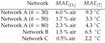
Table 2. Summary of the performance for the three types of neural networks
Network MAE[O2] MAE[T]
Network A ( ˆn=30) 6.0 % air 9.3◦C
Network A ( ˆn=50) 1.7 % air 3.3◦C
Network A ( ˆn=80) 2.3 % air 4.3◦C
Network B 1.5 % air 6.5 ◦C
Network C 0.5% air 2.2 ◦C
The results of Table2show that a simple FFNN as network A is not suitable to extract the two
267
quantities of interest at the same time with good accuracy, since it is not flexible enough. The reason is
268
that the two predicted quantities will depend on the same set of features generated by the hidden layers
269
of network A. When network A tries to learn better weights to predict, for example, the temperature,
270
these will, however, influence also the[O2]prediction and vice-versa. So the common set of weights
271
that are learned can not be optimized for each quantity separately at the same time. The MTL network
272
B tries to address this problem with a separate branch task-specific of layers for[O2]. The tests show
273
however that this architecture is only marginally better for the prediction of[O2]and even worse for
274
the prediction ofT. This is probably due an insufficient flexibility of the network and shows that
275
even if only one parameter were of interest, e.g.,[O2]one single additional branch is not sufficient. A
276
significant improvement is achieved with the MTL network C: the two task-specific branches give the
277
network the flexibility of learning a set of weights (the ones in the branches) specific to each quantity,
278
therefore achieving exceptionally good predictions on both[O2]andT. Note that in this work the
279
hyper-parameter tuning [15] for each network was not performed since the goal is not to achieve the
280
lowest possibleMAEs but rather to demonstrate the advantages and potential of MTL compared to
281
classical FFNN approaches. For the implementation in a measuring instrument, therefore,a further
282
phase of parameter tuning specifically dependent on the application would be needed.
283
6. Conclusions
284
In this work, different neural networks architectures were investigated to solve the problem of
285
extracting multiple separate physical quantities at the same time from a single dataset. This type of
286
multi-dimensional regression problems in physics can be challenging or impossible to solve if the
287
mathematical models describing the functional dependence of the dependent variable from a set of
288
independent variables are too complex or unknown.
289
The proposed approach consists in using neural network MTL architectures, which are
290
characterized by a common set of layers and then task-specific layers for each quantity to be determined.
291
Thanks to the additional task-specific hidden layers this type of network can be trained to perform
292
better than conventional FFNNs when the quantities to be predicted are characterized by a significant
293
difference in physical behavior. The approach is demonstrated by applying it to oxygen luminescence
294
sensing application. The conventional methods rely on a separate temperature determination which
295
is then used as input to correct the extraction of the oxygen concentration from a dataset. This work
296
demonstrates how it is possible to extract from a single dataset of phase shift measurements both
297
the oxygen concentration and the temperature of the medium. In other words, from one single
298
measurement, it is possible to determine two physically different quantities, one of which is dependent
299
from the other. The distributions of AE[O2] and AET are significantly narrower and much more
300
concentrated around zero with the proposed MTL network (type C), as compared to FFNNs without
301
specific and dedicated layers for each Tor [O2] since the predictions are only based on common
features (the ones generated by the common layers) that fail to be flexible enough to describe bothT
303
and[O2].
304
This work aims to open the road to new ways of extracting multiple physical quantities from a
305
common set of data at the same time to achieve consistent results that are both accurate and stable. The
306
described approach is relevant for many practical applications in sensor science and demonstrates that
307
MTL architectures have the potential of revolutionizing the approach to non-linear multi-dimensional
308
regression.
309
Author Contributions:conceptualization, Umberto Michelucci and Francesca Venturini; methodology, Umberto
310
Michelucci; software, Umberto Michelucci; writing, Umberto Michelucci and Francesca Venturini; physics model
311
and examples, Francesca Venturini
312
Funding:This research received no external funding.
313
Acknowledgments:In this section you can acknowledge any support given which is not covered by the author
314
contribution or funding sections. This may include administrative and technical support, or donations in kind
315
(e.g., materials used for experiments).
316
Conflicts of Interest:The authors declare no conflict of interest.
317
Abbreviations
318
The following abbreviations are used in this manuscript:
319
320
FFNN Feed-forward neural networks MTL Multi-task learning
MSE Mean square error AE Absolute error MAE Mean average error KDE Kernel density estimate
321
References
322
1. Nocedal, J.; Wright, S.J.Numerical Optimization, Glynn, P.; Robinson, S.M. Eds.; Springer-Verlag: New York,
323
Inc, 1999.
324
2. Boyd, S.P.; Vandenberghe, L.Convex Optimization (pdf); Cambridge University Press; p. 129.
325
3. James, G.; Witten D.; Hastie, T.; Tibshirani, R.An Introduction to Statistical Learning; Springer: New York,
326
USA, 2013.
327
4. Borisov, S.M. Fundamentals of Quenched PhosphorescenceO2 Sensing and Rational Design of Sensor
328
Materials. InQuenched-phosphorescence Detection of Molecular Oxygen; Papkovsky, D.B, Dmitriev, R.I.,
329
Eds. 2018; pp. 1-18.
330
, 2018. Fundamentals of Quenched Phosphorescence O2 Sensing and Rational Design of Sensor Materials. In
331
Quenched-phosphorescence Detection of Molecular Oxygen (pp. 1-18).
332
5. Baleizão, C.; Nagl, S.; Sch´’aferling, M.; Berberan-Santos, M.N.; Wolfbeis, O.S. Dual Fluorescence Sensor for
333
Trace Oxygen and Temperature with Unmatched Range and SensitivityAnal. Chem.2018,80, 6449–6457.
334
6. Collier, B.B.; McShane, M.J. Simultaneous, accurate lifetime determination of two luminophores using
335
time-domain techniquesSENSORS, IEEE2011, 943–946.
336
7. Pérez de Vargas-Sansalvador, M.; Martinez-Olmos, A.; Palma, A.J. ; Fernández-Ramos, M.D.; Capitán-Vallvey,
337
L.F. Compact optical instrument for simultaneous determination of oxygen and carbon dioxideMicrochimica
338
Acta2011,172, 455–464.
339
8. Lam, H.; Rao, G.; Loureiro, J.; Tolosa, L. Dual Optical Sensor for Oxygen and Temperature Based on the
340
Combination of Time Domain and Frequency Domain TechniquesTalanta2011,84, 65–70.
341
9. A novel planar optical sensor for simultaneous monitoring of oxygen, carbon dioxide, pH and temperature
342
Borisov, S.M.; Seifner, R.; Klimant, I.Analytical and Bioanalytical Chemistry2011,400, 2463–2474.
343
10. Zhang, Y.; Yang, Q. A Survey on Multi-Task LearningarXiv preprint arXiv:1707.081142018, 1–20.
344
11. Thung, K.H.; Wee, C.-Y. A brief review on multi-task learningMultimed. Tools Appl.2018,77, 29705–29725.
345
12. Thrun, S. Is learning the n-th thing any easier than learning the first?Adv. Neural Inf. Process. Syst.1996,8,
346
640–646.
13. Baxter, J. A model of inductive bias learning.Journal of Artificial Intelligence Research2000,12, 149–198.
348
14. Caruana, R. Multi-task learningMachine Learning1997,28, 41–75.
349
15. Michelucci, U.Applied Deep Learning - A Case-Based Approach to Understanding Deep Neural Networks;
350
Apress Media, LLC: New York, NY, USA, 2018; pp. 374–375.
351
16. Irie, B.; Miyake, S. Capabilities of three-layered perceptrons. In Proceedings of the IEEE International
352
Conference on Neural Networks, San Diego, CA, USA, July 1988; pp. 641–648.
353
17. Hornik, K.; Approximation Capabilities of Multilayer Feedforward Networks,Neural Networks,1991Vol. 4,
354
pp. 251-257
355
18. Cybenko, G.Approximation by Superpositions of a Sigmoidal Function1989,2, 303–314.
356
19. Hanin, B. Universal Function Approximation by deep nueral nets with bounded width and relu activations
357
arXiv preprint arXiv:1708.026912017, 1–9.
358
20. Lu, Z.; Pu, H.; Wang, F.; Hu, Z.; Wang, L. The expressive power of neural networks: A view from the width.
359
In 31st Conference on Neural Information Processing Syxstems, Long Beach, CA, USA, 2017; pp. 6231-6239.
360
21. Rojas, R.,Neural Networks - A systematic Introduction; Springer-Verlag Berlin: Heidelberg, 1996; pp.
361
267–271.
362
22. Bishop, C.M.Neural Networks for Pattern Recognition; Oxford University Press: Norfolk, UK, 2005; pp.
363
139–140.
364
23. Sprecher, D. On the structure of Continuous Functions of Several VariablesTransactions of the American
365
Mathematical Society1964,115, 340–355.
366
24. Argyriou, A.; Evgeniou, T.; Pontil, M. Multi-task feature learning. In Proceedings of the 19th International
367
Conference on Neural Information Processing Systems (NIPS’06); B. Schölkopf, J. C. Platt, J. C., Hoffman, T.
368
Eds.; MIT Press: Cambridge, MA, USA, 41–48.
369
25. Kingma, D.P.; Ba, J. Adam: A method for stochastic optimization.arXiv preprint arXiv:1412.69802014, 1–15.
370
26. Wang, X.-D.; Wolfbeis, O.S. Optical methods for sensing and imaging oxygen: materials, spectroscopies and
371
applications.Chem. Soc. Rev.2014,43, 3666–3761.
372
27. Narayanaswamy, R.; Wolfbeis, O.S. Eds. Optical sensors: Industrial Environmental and Diagnostic
373
Applications, 1st ed; Vol. 1. Springer Science & Business Media: Berlin, Germany, 2004; pp. 28–30.
374
28. Lakowicz, J. R.Principles of Fluorescence Spectroscopy, 3rd ed.; Springer: Singapore, 2006.
375
29. Demas, J.N.; DeGraff, B.A.; Coleman, P.B. Oxygen Sensors Based on Luminescence Quenching.Anal. Chem.
376
1999,71, 793A–800A.
377
30. Michelucci, U.; Baumgartner, M.; Venturini, F. Optical oxygen sensing with artificial intelligenceSensors
378
2019,19, 777.
379
31. Burnham, K. P.; Anderson, D. R., Model Selection and Multimodel Inference, 2nd ed., New York;
380
Springer-Verlag, 2002
![Figure 5. Absolute error AE[O2] in the prediction of the O2 concentration for the different concentrationranges using network A](https://thumb-us.123doks.com/thumbv2/123dok_us/7910983.1313528/8.595.79.514.567.723/figure-absolute-error-prediction-concentration-different-concentrationranges-network.webp)
![Figure 7. Kernel density estimation for AE[O2] with network A. Left: 30 neurons per hidden layer;middle: 50 neurons per hidden layer, right: 80 neurons per hidden layer.](https://thumb-us.123doks.com/thumbv2/123dok_us/7910983.1313528/10.595.72.514.511.665/figure-kernel-density-estimation-network-neurons-neurons-neurons.webp)
![Figure 10. Kernel density estimation for AE[O2] for networks A (left), B (middle), and C (right).](https://thumb-us.123doks.com/thumbv2/123dok_us/7910983.1313528/11.595.80.514.600.732/figure-kernel-density-estimation-networks-left-middle-right.webp)