Thesis by
Emerson Cristian Melo Sanchez
In Partial Fulfillment of the Requirements for the Degree of
Doctor of Philosophy
California Institute of Technology Pasadena, California
2013
c 2013
Acknowledgements
The past five years at the Humanities and Social Sciences Division at Caltech have been an amazing experience, both intellectually and socially. The students, faculty and staff make a friendly and motivating environment. I specially thank Laurel Aucherpanchag and Nilanjan Roy.
I am deeply in debt to my advisor Federico Echenique. His guidance played a fundamental role in the completion of this thesis. Federico shared his experience and was patient enough until I got decent research problems. Our weekly meeting has been a fascinating learning experience in my career.
I also thank my committee members Leeat Yariv, Matthew Shum, and Robert Sherman. From Leeat I have learned how to present and explain results in a clear and easy way. I thank Bob and Matt for the many hours that they spent with me in discussing about research problems, just for the pleasure of learning new things.
I deeply thank my Master thesis’ advisor Roberto Cominetti, for encouraging me to pursue Doctoral studies. Despite not being a mathematician, Roberto generously accepted to be my guide and through many hours of discussions he taught me how to do research. Roberto is my model to follow as a scientist.
meetings have influenced the way that I understand economic theory.
My two wonderful friends Sandra and Jorge, have supported me during the pro-cess the my graduate studies. They always have been there for me. I thank Sandra for her friendship all of these years, and for her unconditional support on my career. I thank Jorge for his generosity in reading the drafts of the chapters of this thesis, and for his unconditional support since we met in the calculus class; I still remember his tough questions in that class.
Finally, thanks are due to my family, who are everything. To my brother Jhonny for his love and unconditional support, and for the many hours talking on the phone about the “pez”, which helped me to release the stress of hard days in the researching process. To my sister Maria Jose for her love, unconditional support, and for giving me my adorable little niece Monserrat. To my brother in law David for his constant support since we met. To my wonderful fiance and best friend Xinia for her immense love and support, and with whom I get to share the many upcoming adventures in our lives. Xinia has showed me that the life is more than equations and models. To the babies, Azul and Santino for making my life special, and for accepting as a member of their family.
Abstract
Contents
Acknowledgements iv
Abstract vi
1 Introduction 1
2 Bargaining and centrality in networked markets 4
2.1 Introduction . . . 4
2.1.1 Outline of the model . . . 7
2.1.2 Related work . . . 9
2.2 The model: exchange networks . . . 10
2.3 Market equilibrium and eigenvector centrality . . . 19
2.4 Seller-buyer networks . . . 21
2.4.1 Seller-buyer networks and eigenvector centrality . . . 26
2.5 Conclusions . . . 28
3 A representative consumer theorem for discrete choice models in networked markets 29 3.1 Introduction . . . 29
3.3 Main result . . . 35
3.3.1 The sequential logit case . . . 37
3.4 Applications . . . 38
3.4.1 Price competition in parallel serial link networks . . . 39
3.4.2 Merging analysis . . . 45
4 Price competition, free entry, and welfare in congested markets 48 4.1 Introduction . . . 48
4.1.1 Our contribution . . . 50
4.2 The Model . . . 54
4.2.1 Markovian traffic equilibrium . . . 56
4.2.2 Existence and uniqueness of an MTE . . . 62
4.3 Oligopoly pricing: existence and uniqueness of a symmetric price equi-librium . . . 64
4.3.1 Welfare analysis and entry decisions . . . 66
4.4 Existence and uniqueness of an OE: The general case . . . 70
4.4.0.1 Existence . . . 71
4.4.0.2 Uniqueness . . . 74
4.5 Conclusion and final remarks . . . 80
A Appendix to Chapter 1 81 A.1 Definitions and proofs . . . 81
A.1.1 Definitions . . . 81
A.1.2 Proof of Theorem 2 . . . 82
B Appendix to Chapter 2 86
B.1 Proofs . . . 86
B.2 Appendix: Sequential MNL and its relationship with the nested logit model . . . 88
C Appendix to Chapter 3 91 C.1 Proofs . . . 91
C.1.1 Quasi concavity of the profit function . . . 92
C.1.2 Analysis of C−a(pOE) . . . 95
C.1.3 Analysis of the existence and uniqueness of an OE . . . 97
List of Figures
2.1 A network with seven players and six links . . . 19
2.2 A network with two sellers and two buyers . . . 25
2.3 A network with two sellers and two buyers . . . 26
3.1 Cournot’s complements model . . . 41
3.2 A parallel serial link network . . . 43
3.3 The effect of adding a serial link . . . 44
3.4 A network of complements and substitutes . . . 46
Chapter 1
Introduction
This thesis belongs to the growing field of economic networks. In particular, we develop three essays in which we study the problem of bargaining, discrete choice representation, and pricing in the context of networked markets. Despite analyzing very different problems, the three essays share the common feature of making use of a network representation to describe the market of interest.
We point out that the eigenvector approach is a way of finding the most central or relevant players in terms of the global structure of the network, and to pay less attention to patterns that are morelocal. Mathematically, the eigenvector centrality captures the relevance of players in the bargaining process, using the eigenvector associated to the largest eigenvalue of the adjacency matrix of a given network. Thus our result may be viewed as an economic justification of the eigenvector approach in the context of bargaining in networked markets.
As an application, we analyze the special case of seller-buyer networks, showing how our framework may be useful for analyzing price dispersion as a function of sellers and buyers’ network positions.
From a technical viewpoint, we show how simple ideas from the theory of linear complementarity problems can be exploited in the context of networked markets and Nash bargaining. In particular, we show that both models, the exchange network and the seller-buyer networks, can be analyzed through the study of an associated quadratic optimization problem. This optimization problem encapsulates all the needed information to understand existence, uniqueness, and characterization of a market equilibrium.
show that a demand system for hierarchical or sequential decision processes can be obtained as the outcome of utility maximization by a representative agent. We only require the mild condition that the distribution of the unobserved components must be absolutely continuous.
From an applied perspective we point out that our results can be useful for carrying out welfare analysis in networked markets, where the standard discrete choice theory may not apply. For example, our results can be applied to bundling decisions, merger analysis, or compatibility among goods in networked markets.
Chapter 2
Bargaining and centrality in
networked markets
2.1
Introduction
Traditional models of economic exchange assume that all possible coalitions of agents can meet and trade. However, due to social relationships, institutional, legal, and physical barriers, it may be impossible for certain sets (pairs) of sellers and buyers to communicate or trade with one another directly. For example, financial markets, supply chains, international trade, and many other markets exhibit barriers limiting the kinds of coalitions that agents may form.
A simple way of capturing the barriers to the exchange process is via the network of connections/exchanges it allows for trading. Formally, in a given network the set of nodes represent players and the set of links represent the possibilities of exchange between any two players. Thus, the use of a network representation has the advantage of showing in a simple way how the different types of barriers to trade determine different market structures.
payoffs. We focus on the following key question:
How does network topology determine players’ payoffs (market outcomes)? We address the question by studying a simple bargaining model in networked markets. Our model is based on random matching and theNash bargaining solution, and has the advantage of being simple, and most importantly, providing an explicit connection between players’ network positions and equilibrium payoffs. Concretely, we show that players’ equilibrium payoffs are uniquely determined by their degree of centrality in the network, measured by Bonacich [1987]’s centrality measure.1
Our characterization shows how payoffs dispersion is driven by players’ network positions, where players with a higher degree of centrality obtain higher payoffs than players with lower centrality. Thus players’ positions determine their market power in the trading process.
In addition, we note that our result can be seen as economic justification of Bonacich’s measure in the context of bargaining in networked markets. 2
Our second contribution is the result that as long as the players’ discount factor goes to one, the equilibrium payoff vector converges to the eigenvector centrality.
We point out that the eigenvector approach is a way to find the most central or relevant players in terms of the “global” structure of the network, and to pay less attention to patterns that are more “local”. Mathematically, the eigenvector central-ity captures the relevance of players in the bargaining process, using the eigenvector associated to the largest eigenvalue of the adjacency matrix of a given network.3
1For a survey of applications of Bonacich’s measure in economics we refer the reader to Jackson
[2008] and Goyal [2009].
2In fact, Bonacich [1987] proposes the measure as way to rationalize the outcome of lab
experi-ments in the context of bargaining in networks, but without considering an economic model.
3From an applied perspective, the eigenvector approach has been applied in sociology and in the
Thus our result may be viewed as an economic justification of the eigenvector approach in the context of bargaining in networked markets.
Formally, our convergence result relies on the specific relationship between, the discount factor, the matching technology, and the network structure, and intuitively it may be interpreted as follows: as long as players become more and more patient, then the market equilibrium is driven by the eigenvector centrality.
We remark that our result is not the first establishing the connection between Bonacich’s measure and the eigenvector centrality. 4 However, the main contribution
of our result is that it provides a simple and intuitive economic condition for under-standing when Bonacich’s measure can be interpreted as the eigenvector centrality
As a particular case of our model, we analyze the problem of seller-buyer net-works. For this specific environment, we show that a convex minimization problem contains all the relevant information to study existence and uniqueness of a market equilibrium. The characterization of a market equilibrium as the solution of a mini-mization problem turns out to be useful in the context of networks with finitely many sellers and buyers, where standard procedures of convex optimization may be imple-mented. Furthermore, we exploit the bipartite structure of seller-buyer networks in order to provide an explicit characterization of equilibrium payoffs in terms of sellers and buyers’ positions. This characterization rationalizes why buyers with the same valuation for a good may, in equilibrium, pay different prices.
For the case of the convergence of a market equilibrium to the eigenvector cen-trality, we show that for sellers and buyers two mutually exclusive conditions can be derived. The reason for this different condition is given by the bipartite structure of
4See for example Friedkin and Johnsen [1990], Friedkin [1991], Bonacich [1997], and Bonacich
seller-buyer networks.
It is worth remarking that our result of payoffs characterization as the conver-gence of a market equilibrium to the eigenvector centrality extend the findings in Corominas-Bosch [2004]. Concretely, our results fully characterize the sellers and buyers’ payoffs in terms of networks positions without relying on a specific bargain-ing protocol, whereas Corominas-Bosch [2004]’s results rely on the kind of bargainbargain-ing protocol implemented.
From a technical viewpoint, we show how simple ideas from the theory of linear complementarity problems can be exploited in the context of networked markets and Nash bargaining. In particular, we show that both models, the exchange network and the seller-buyer networks, can be analyzed through the study of an associated quadratic optimization problem. This optimization problem encapsulates all the needed information to understand the existence, uniqueness, and characterization of a market equilibrium.
2.1.1
Outline of the model
Our model may be described as follows. We consider an environment in which any pair of players can trade if and only they are connected in the network. The network represents the underlying social structure, where a link between two players represents the opportunity to create one unit of surplus. Given the possibility of jointly creating such surplus, both players (connected by a link) must agree on how to split it. We assume that players split the surplus according to thesymmetric Nash bargaining solution.5
Borrowing ideas from the macroeconomics literature on search, we model the
5The symmetry assumption is made for simplicity, but it is not essential to our analysis. In fact,
meeting process among players in dynamic and random way. In particular, at each point of time, a link connecting two agents is randomly drawn.6Then the chosen
players must split the surplus (according to the Nash bargaining solution). An important feature is that the disagreement points are determinedendogenously. This endogeneity captures the fact that if two chosen players do not reach an agreement, then they can wait until the next period with the expectation of being drawn again and so achieve a better payoff.7 On the other hand, if two players reach an agreement,
then they split the surplus and leave the market, and their positions in the network are occupied by two new players.8 Players discount utilities using a common discount
factor.
This random exchange process induces a dynamical system which shows how players’ payoffs evolve over time. In order to study the equilibrium of the exchange process, we analyze its steady state, which we refer as amarket equilibrium.
In this framework, it is easy to show the existence and uniqueness of a market equilibrium. However, the most important property of our analysis is the fact that a market equilibrium is exactly equivalent to the centrality measure proposed by Bonacich [1987]. For this characterization, we provide a condition such that the market equilibrium converges to the eigenvector centrality.
6It is worth remarking that the idea of drawing a link at random at each point of time was
early proposed in Stolte and Emerson [1977] in the context of experiments on exchange networks in sociology. Thus our choice of the matching technology can be justified from an experimental perspective.
7The endogeneity of the disagreement points allows us to link the Nash’ bargaining solution
with the strategic approach. See Binmore et al. [1986] for a detailed discussion about this technical aspect.
8This assumption allows us to avoid strategic considerations that would be raised in the situation
2.1.2
Related work
The model we have described in the previous section is related to two different branches of economic literature. Specifically, our model is related to macroeconomics models of search and matching9, and models of bargaining in networked markets.10
Instead of describing the extensive literature on these different approaches, we shall describe the paper by Manea [2011], which turns out to be the closest article to our work.
The paper by Manea [2011] develops a model of strategic bargaining in networked markets. In particular, Manea [2011] extends Gale [1987]’s strategic approach to network environments. However, there are two important differences between our paper and Manea [2011]’s approach. First, we analyze a networked market using the symmetric Nash bargaining solution, whereas Manea [2011] proposes a strategic model where the extensive form of the bargaining turns out to be critical. Formally, in Manea [2011] there are many possible sub game perfect Nash equilibria supporting a market outcome. Because we use the Nash bargaining solution we get rid of this multiplicity problem.
The second and most important difference, is that our approach allows us to give a simple and explicit expression for the equilibrium payoff vector in terms of Bonacich [1987]’s centrality measure. Furthermore, we are able to derive an economic condition to relate Bonacich’s measure with the eigenvector centrality in the context
9The idea of combining random matching and Nash bargaining was first proposed in the
macroe-comomic literature on search. The first papers proposing this approach were Diamond and Maskin [1979] and Diamond [1982]. A survey of this literature can be found in Rogerson et al. [2005].
10Two early papers that analyze markets using a network representation are Kranton and
of bargaining in networked markets. Neither of these results are in Manea [2011]. The rest of the chapter is organized as follows. Section 4.2 describes the basic model of exchange in networks. Section 4.3 analyzes the relationship between our market equilibrium and the eigenvector centrality. Section 4.4 studies the specific case of sellers-buyers networks. Section 2.5 concludes. Definitions and proofs are relegated to Appendix A.1 .
2.2
The model: exchange networks
Let N = {1, . . . , n}, with n ≥ 3, being the set of agents, and let i and j denote typical members of this set. LetE ⊂N×N be the set of connections (relationships) among agents in N. Given the sets N and E, we define a networked market by the undirected graphG= (N, E). We identify the networkG with its adjacency matrix G= (gij), wheregij = 1 if there is a link betweeniandj, andgij = 0 otherwise. We
denote byGN the set of all possible networks given the set of agentsN. In particular,
a link ij ∈G is viewed as the ability of agents i and j to generate a unit of surplus. We shall assume that any pair of agents in the networkG, can be connected through a collection of links in E. Formally, we shall assume that any network G ∈ G is strongly connected.
For each playeri∈N, we define the set of neighbors asNG
i ={j ∈N : ij ∈G},
which describes the set of agents with which playerican meet and trade. We denote the cardinality of NG
i as di = |NiG|. We refer to di as agent i’s degree, where the
diagonal matrix D contains the degree of all players, i.e., its elements are given by the di.
bargaining process. Each period of time t = 0,1, . . . , a link ij ∈ G is selected randomly with an exogenous probability πij. The probability πij is the probability
that agents i and j are drawn to trade. We assume the πijs are uniform, with
πij = π = E1 for all ij ∈ G. We shall refer to the probability measure π as the
matching technology.11
Once the link ij is drawn, players iand j split the generated surplus accordingly to the Nash bargaining solution. Players discount payoffs with a common discount factor 0< δ <1.
From the previous description, the dynamical process can be summarized as fol-lows. At timetplayersiandj, connected through linkij, are chosen with probability
π to bargain over one unit of surplus. If they do not reach an agreement, each stays in the market until t+ 1, waiting for a new opportunity to trade. In the case that both players reach an agreement at time t they split the surplus using the Nash solution. We point out that the disagreement points for players i and j correspond to they expected utility if they remains in the market until periodt+ 1. In order to analyze a steady state situation, we assume that when a pair of playersiandj reach an agreement, they leave the market, and they are replaced in the same positions by two new players.
In a steady state situation, let Vi be player i’s steady state expected payoff of
being in the market at time t. Then if at time t the pair of players i and j fail to reach an agreement, they remain in the market until timet+ 1, and from the point of view of timet, disagreement results in expected utilitiesδVi and δVj.
Formally, a steady state is represented by the following system of linear equations:
11We point out that this type of matching technology on networks was early proposed in the
Vi =
X
j∈NG i
π
2(1−δVj +δVi) + (1−diπ)δVi, ∀i. (2.1)
The explanation for equation (2.1) is the following. When players i and j are drawn to trade, they split the surplus, and thanks to the Nash bargaining solution, player i gets 1
2(1−δVj+δVi). Because the meeting between players i and j occurs
with probabilityπ, we find that the expected payoff for player iis π2(1−δVj+δVi).
Adding up over allj ∈NG
i , we find that player i’s expected value of being drawn at
time t isP
j∈NG i
π
2(1−δVj +δVi). The second term is due to the fact that at time t
with probability (1−diπ), playerihas to wait till period t+ 1 for a new opportunity
to trade. The expected value of this event is (1−diπ)δVi. Combining these two
expected values we get expression (2.1).
Equation (2.1) can be written in a compact way using matrix notation. In par-ticular, we get the following
(1−δ)[I+πκA]V = π
2d, (2.2)
where A = D +G, a n-square matrix, and d = (di)i∈N the n−dimensional
de-gree vector. The parameter κ is defined as κ = δ
2(1−δ). Finally V = (Vi)i∈N is an
n−dimensional vector, which captures players’ payoffs. Expression (2.2) may be rewritten as:
where W≡[I+πκD]−1G and ˆc= 1
(1−δ)[I+πκD]
−1c= 1
2(1−δ)W1, with 1 a vector
of ones. It is worth nothing that the matrix W can be interpreted as a weighted adjacency matrix.
We now are ready to give a definition of a market equilibrium for the networked market just described.
Definition 1 A payoff vectorV∗ is a market equilibrium (ME) if it solves (2.3) with
V∗
≥0.
In other words, Definition 1 establishes that a nonnegative solution of (2.3) is an ME. The intuition for V∗
≥ 0 is that players can afford zero payoffs if they decide not to participate in the market. Thus the non negativity condition for a ME can be interpreted as an individual rationality condition.
Our first task, is to establish that such an ME exists. In order to analyze the existence and uniqueness of a ME, we borrow basic ideas from the theory of linear complementarity problems (Cottle et al. [2009]). The application of this technique is based on the the observation that a ME can be formulated as the following collection of linear inequalities:
V ≥ 0 (2.4)
(I+πκW)V −ˆc ≥ 0 (2.5)
VT([I+πκW]V −ˆc) = 0 (2.6)
where a vectorV is a solution to a ME, if and only if V satisfies (2.4)-(2.6) simulta-neously. For short, we refer to (2.4)-(2.6) as LCP(W,ˆc).
Proposition 1 below states the simple but important fact that the ME can be analyzed as the solution of LCP(W,ˆc).
Proposition 1 V∗ is an ME if and only if V∗ solves the
LCP(W,c).ˆ
The main advantage of studying the equilibrium problem through LCP is the powerful battery of results of existence and uniqueness of solutions. In fact, our next result exploits such connection.
Proposition 2 There exists a unique ME which is given by the solution of the fol-lowing optimization problem:
minV {
1 2V
TMV
−cTV} (2.7)
s.t. V ≥0,
with M= (1−δ)[I+πκD][I+πκW].
stress that despite of its apparently similarity with the sort of problems analyzed in Bramoulle et al. [2011], their results do not apply to our problem.
Our second task is to establish the connection between network topologies and equilibrium payoffs. In order to provide a characterization of the equilibrium payoffs in terms of network topologies, we need to introduce the notion of centrality measure. Our next definition introduces Bonacich’s centrality measure.
Definition 2 (Bonacich [1987]) Let G ∈ GN, and let H be its (non negative)
weighted adjacency matrix. Let µ ∈ R be such that K(µ,H) = [I−µH]−1 is well
defined and nonnegative. Letθ ∈Rn+. The vector of (weighted) Bonacich centralities
of parameter µ for the matrix H is given by:
b(µ,H;θ) =K(µ,H)·H·θ.
In Definition 2, the parameterµreflects the degree to which a player’s payoff is a function of the payoffs of those to whom he is connected. Ifµis positive,b(µ,H;θ) is a conventional centrality measure in which each player’s payoff is a positive function of the payoffs of the players with which it is in contact. When µ is negative, each player’s payoff is reduced by the higher payoffs to those to which it is connected.
We point out that Bonacich’s measure was first applied in economics by Ballester et al. [2006] in the context of network games. In sociology, Bonacich’s measure is widely used in empirical and experimental work.12 To the best of our knowledge, in
the context of bargaining in networked markets, no previous paper has characterized the equilibrium in terms of Bonacich’s measure
Theorem 1 The equilibrium payoff vector V∗ satisfies:
V∗ =b(−πκ,W; ˆc), (2.8)
where cˆ= 1
2(1−δ)W·1.
In order to explain the economic intuition of Theorem 1, we may rewrite (2.8) as follows:
V∗ = ˆc−πκWV∗, (2.9)
V∗ = [I
−πκW]ˆc | {z }
Local Effect
+ (πκ)2W2V∗
| {z }
Global Effect
. (2.10)
Equations (2.9) and (2.10) show how players’ payoffs depend on the whole network structure. For example equation (2.9) shows how players’ payoffs depend negatively on the amount of share of surplus that players must give to their direct neighbors. In addition, Equation (2.10) shows that the payoff characterization in Theorem 1 can be decomposed into local and global effects. The term [I−πκW]ˆc shows the effect of direct links on players’ payoffs. However, the interesting term is (πκ)2W2V∗,
which shows how the indirect links have a positive effect on players’ payoffs. For example, if we consider playeri, then (πκ)2W2
V∗ shows how the links of players in
the setNG
i (playeri’s neighbors) have a positive effect on his equilibrium payoff. The
intuition for the global effect captured by (πκ)2W2
V∗, is that from player i’s point
of view, it is better if her neighbors inj ∈NG
i are connected to players that demand
a large share of the surplus. For example, we can think of the situation where the set of n buyers is connected to one common seller, i.e., the market is supplied by a monopolist. It follows that buyers do not have connections to other possible sellers, so the monopolist can exploit this fact in the bargaining process demanding a large share of the surplus. In this case, Theorem 1 predicts that the monopolist gets almost all the surplus.
In the previous analysis, the key element for deriving our intuitions is the negative term −πκ. Concretely, the fact that −πκ <0 means that V∗ is reduced when the
connections of any player are themselves central (equation (2.9)), but increased by the centrality of those at distance two (equation (2.10)), whose centrality has reduced the centrality of those at distance one. Thus, a player can have bargaining power because his neighbors have no options (alternative players to trade) or because his neighbors are connected to players with a high degree of centrality.
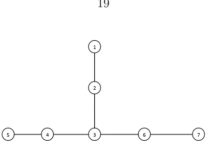
In order to understand the utility of our caractherization, let us consider the network in Figure 2.1, which consists of seven players and six links. Because we are assuming that the matching technology is uniform, we get π = 16. For the case of
δ= 0, we get thatπκ= 0, and the equilibrium payoffs areV∗
1 =V5∗ =V7∗ = 0.08 and
V∗
2 =V4∗ = V6∗ = 0.17, and V3∗ = 0.25. In this case players’ payoffs are determined
direct links, and the network topology does not play any role. However, for values of
δ in the open interval (0,1), payoffs behave in a different way. In fact, for δ = 0.99, we get that πκ > 0, which implies V∗
5 = V7∗ = 0.41, V2∗ = V4∗ = V6∗ = 0.55, and
V∗
3 = 0.44. In other words, for δ = 0.99 we get
V2∗ =V4∗ =V6∗ > V3∗ > V5∗ =V7∗.
1
2
3 6 4
5 7
Figure 2.1: A network with seven players and six links
2.3
Market equilibrium and eigenvector centrality
The example in Figure 2.1 shows how players’ equilibrium payoffs depend on the value of the discount factor δ. In particular, example 2.1 shows that when the discount factor δ goes to one, players’ payoffs depend on the whole network structure.
In this section we show that a general conclusion can be obtained for the case when the discount factorδ goes to one. In order to estate our convergence result, we need to introduce some notation. We denote the maximum eigenvalue (in absolute value) of the matrix A by ρ(A). Let e and q be the left and right eigenvectors associated to ρ(A).
We remark that, thanks to Perron-Frobenius’ Theorem (Ch. 8, Horn and Johnson [1990]), we get thatρ(A)>0, and the eigenvectoreis strictly positive and uniquely determined (up to constant).
Definition 3 Let G ∈ GN, and let H be a non negative matrix induced by the
network G. The eigenvector centrality e(H) of the matrix H is its right eigenvector associated to the spectral radius ρ(H).
The previous definition states that the eigenvector centrality is the right eigen-vector associated to the largest eigenvalue of a matrix H. In terms of our problem, the matrix H is given by the matrix A, which is just the adjacency matrix plus the diagonal matrix D.
Now we are ready to establish the main result of this section.
Theorem 2 Let V∗ be a market equilibrium, and let W∗ ≡Pn
i=1Vi∗. Then
lim
δ↑ 1
πρ(A)/2+1
V∗
W∗ =e(A).
We note that Theorem 2 shows the explicit relationship among π, the discount factorδ and the networkG. In particular, the conditionδ−→ 1
πρ(A)/2+1 provides an
economic condition to establish the connection between our ME given by Bonacich’s measure and the eigenvector centrality. Thus Theorem 2 has the economic inter-pretation that as long as the discount factor goes to one the ME is driven by the eigenvector centrality.
is that we show that a simple economic condition on the discount factor contains all the relevant information about the relationship between Bonacich’s measure and the eigenvector approach. Furthermore, our result can be seen as an economic justifica-tion to the eigenvector centrality.
Proposition 3 below shows that for the case of regular networks a sharper condi-tion may be obtained, which establishes that the number of players plays a role in the convergence. We recall that a network G is called regular of degree d if di =d
for all i∈N.
Proposition 3 LetGbe a regular network of degreed. Then limδ↑ 1 1/n∗+1
V∗
W∗ =e(A),
where n∗ = n 2.
The previous result shows how the number of players, in the case of regular networks, plays an important role. In particular, for the case of networks with finitely many players, we may expect 1
n∗ to be close to zero, so that the condition
δ−→ 1
1/n∗+1 can be viewed as δ−→1.
2.4
Seller-buyer networks
buyer network, allows us to characterize an ME in terms of two vectors, which capture sellers and buyers’ payoffs, respectively.
Proposition 5 Let V∗
S and VB∗ be the sellers and buyers equilibrium payoff vectors
respectively. Then
VS∗ = b(α,WSB;θSB),
VB∗ = b(α,WBS;θBS),
where α= (πκ)2,W
SB =WS×WB, WBS =WB×WS, and θSB = ˆcS−πκWScˆS,
θBS = ˆcB−πκWSˆcS, with cˆl = [Il+πκGl]−1cl for l=S, B.
Proposition 5 characterizes sellers’ (respectively buyers’) payoffs in terms of their network positions. Concretely, Proposition 5 shows how an ME is determined by Bonacich’s centrality measure. Thus, for the particular case of seller-buyer networks, Bonacich’s measure can be viewed as a measure of market power, which is driven by sellers and buyers’ positions.
Example 1 Let G be the sellers-buyers network displayed in Figure 2.2. Let δ = 0.99 be the value for the discount factor. From Proposition 5, we get the following equilibrium payoffsVs1 = 0.5, Vs2 = 0.48, Vb1 = 0.48, and Vb2 = 0.5. The equilibrium
payoffs show how sellers1and buyerb2 obtain a higher (expected) share of the surplus.
The difference in payoffs is driven by players’ positions. In particular, seller s1 and
buyerb2 can exploit buyerb1 ands2 respectively. In fact, they use their local monopoly
power to extract a higher share of the surplus. In terms of network positions seller
s1
b1 b2
s2
Figure 2.2: A network with two sellers and two buyers
similar reasoning applies to the case of seller s2 and buyer b1, which in terms of
network positions are identical.
Example 2 Let us consider the network displayed in Figure 2.3. The main feature of this network is that each seller (buyer) is connected to the two buyers (sellers) on the other side. Let us assume δ = 0.99. Then the equilibrium payoffs are given
Vs1 = Vs2 = Vb1 = Vb2 ≈ 0.5. The equilibrium payoffs represent the fact that in
s1
b1 b2
s2
Figure 2.3: A network with two sellers and two buyers
It is worth emphasizing that Examples 2.2 and 2.3 show how our framework differs from the approach Corominas-Bosch [2004]. The main difference is the fact that our results do not rely on a specific protocol in the bargaining process, and, most importantly, our approach and results highlight the relevance of sellers and buyers’ network positions.
2.4.1
Seller-buyer networks and eigenvector centrality
In this subsection we show how our convergence result in Theorem 2 may be spe-cialized to the case of seller-buyer networks exploiting the bipartite structure of the network.
Before establishing our result, we need to introduce some notation. Let pS and qS be the right and left eigenvectors of WS respectively. Similarly, let pB and qB
be the right and left eigenvectors of WB, respectively. Let ρ(WS) and ρ(WB) be
the largest eigenvalue of WS and WB, respectively.
2.5
Conclusions
This chapter presents a simple model of bargaining in networked markets. We present two main results. First, we show that the equilibrium payoffs are given by Bonacich [1987]’s centrality measure. Our result may be viewed as an economic justification of this measure in the context of bargaining in networked markets.
Chapter 3
A representative consumer
theorem for discrete choice models
in networked markets
3.1
Introduction
In this Chapter, we propose a way of modeling sequential discrete decision processes, which is consistent with the random utility hypothesis and the existence of a repre-sentative agent. In particular, our approach is based on a network representation for the consumers’ decision process and dynamic programming.1Combining the
afore-mentioned elements, we show that a demand system for hierarchical or sequential decision processes can be obtained as the outcome of the utility maximization by a representative agent. Our result differs from previous findings in two important aspects. First, our result is in terms of a direct utility representation, whilst most of
1The idea of analyzing discrete choice models using a network representation is also considered
results available in discrete choice theory are based on anindirect utility approach.2
Second, and most important, our result does not depend on parametric assumptions concerning the random components associated to the utilities of different choices. From a technical point of view, we need to assume that the random variables are independent within any bundle (path) of goods, but we do not rule out the possibility that the random components can be correlated among different bundles (paths).
Thus, given its generality, our approach and result can be useful in the study of demand systems with complex substitution patterns among the utilities associated with different choices.
An important feature of our result is that when we assume the specific double exponential distribution for the unobserved components, we show that the nested logit model can be seen as a particular case of our approach. In particular, we show that a sequential logit under specific parametric constraints coincides with the nested logit model(McFadden [1978a,b, 1981]).3 This result generalizes previous
findings in Borsch-Supan [1990], Konning and Ridder [1993], Herriges and Kling [1996], Verboven [1996], Konning and Ridder [2003], and Gil-Molto and Hole [2004]. All of these papers impose parametric constraints in order to be consistent with the random utility maximization. Our result shows that such constraints can be avoided using the assumption of sequential decision making.
Finally, from an applied perspective we point out that our results can be useful to carry out welfare analysis in networked markets, where the standard discrete choice theory may not apply. For example, our results can be applied to bundling decisions,
2For a survey of these results see Anderson et al. [1992].
3It is worth pointing out that the nested logit model does not need to be interpreted as a
merger analysis, or compatibility among goods in networked markets.4
The chapter is organized as follows: section 3.2 presents the model, section 3.3 presents the main result of this chapter, and subsection 3.3.1 discusses the logit case. Finally, section 3 applies our demand framework to study price competition and merging in the context of networked markets. Appendix B.1 contains the proofs.
3.2
The model
Let G= (N, A) be an acyclic directed graph with N being the set of nodes and A
the set of links respectively. Without loss of generality, we assume that the graph
G has a single origin-destination pair, where o and t stand for the origin node and destination node respectively.
We identify the set N as the set of decision nodes faced by consumers, and the setA is identified as the set of the available goods in this economy, i.e., the goodais represented by the linka∈A.5 Thus, starting at the origin o, consumers can choose
bundles of goods through the choice of links onA. The destination tis interpreted as the node that is reached once consumers have chosen their desired bundles of goods, and then they leave the market.
For each gooda∈A, consumers’ valuation is represented byθa∈R++. Similarly,
pa∈R+is the price associated to gooda. Thus, the utility for goodamay be written
as ua = θa −pa. We assume that there exists a continuum of users with unitary
mass. According to this, let d = (da)a∈A a non-negative flow vector, where da ≥ 0
denotes the demand for gooda. Any flow vectordmust satisfy the flow conservation
constraints
X
a∈A−i
da =
X
a∈A+i
da ∀i∈N, (3.1)
where A−i denotes the set of links ending at node i, and A+i denotes the set of links starting at nodei. The set of feasible flows is denoted by D.
It is worth emphasizing that in this chapter we interpret each path in the graph as a bundle of goods.6 This interpretation allows us to see the goods within a bundle
as complements, and different paths can be viewed as substitute goods.
In order to introduce heterogeneity into the model, we assume that consumers are randomly drawn from a large population. According to this, the random utility e
ua may be defined as
e
ua=ua+a ∀a∈A+i , i∈N,
with {a}a∈A being a collection of absolutely continuous random variables with E(a) = 0 for all a. The random variables a take into account the heterogeneity
within the population. In particular, these random variables represent the variabil-ity of the valuation θa.
For all nodei6=d, we assume that the random variablesa ∈A+i are independent
with the random variablesb ∈A+ja. In other words, we rule out the possibility that
random variables within the same path can be correlated. Nonetheless, for all i6=d
we allow for correlation among the random variablesa ∈A+i . Furthermore, we allow
for correlation among the random variables in different paths.
6We point out that the standard discrete model can be viewed as particular case of our approach.
In this networked market, consumers choose the optimal bundle of goods in a recursive way. Concretely, at each node consumers choose a good considering their utility plus the continuation value associated to their choices. Formally, at each node
i6=d we define the random utility ˜Va as
˜
Va = Va+a (3.2)
with Va = ua+ϕja(V) and ϕja(V) ≡ E(maxb∈A+ja{Vb +b}), where ja denotes that
nodeja has been reached using the linka.
Regarding equation (3.2) three remarks are important. First, thanks to the as-sumption of independence among the a along the same path, the terms a and
ϕja(·) are independent. Second, equation (3.2) makes explicit the recursive nature
of the consumers’ choice process. In particular, consumers reaching node i observe the realization of the random variables ˜Va, and choose the link a ∈ A+i with the
highest utility, taking into account the current utilityua plus the continuation value
ϕja(V).7The third observation is that (3.2) makes explicit the assumption that a
con-sumer makes sequential choices. In other words, concon-sumers maximize utility solving a dynamic programming problem.8
From previous discussion, it follows that the expected flow xi entering node i
splits among the goodsa ∈A+i according to
7In the discrete choice literature the functionsϕi(
·) are known as theinclusive values at node
i6=d(See McFadden [1978a,b, 1981], Anderson et al. [1992]).
8We point out that the idea of modeling discrete choices through a sequential process was first
Definition 4 Let p≥ 0 be a given price vector. A vector d ∈ R|+A| is a Markovian
assignment if and only if the da’s satisfy the flow distribution equation (3.5) with V
solving Va =ua+ϕja(V) for all a∈A.
We stress that the previous setting defines consumers’ utility in an indirect way. Assuming a specific distribution for the a, we can solve Va =ua+ϕja(V) and find
the demand vector. The next section establishes the main result of this chapter: The Markovian assignment is equivalent to the demand system generated as the solution of adirect utility function by a representative consumer.
3.3
Main result
For the networked market described in section 3.2, we consider there exists a representative consumer endowed with incomeY ∈R++. There is a numeraire good
which is indexed by 0, and its price p0 is normalized to the unity. The budget
constraint for the representative consumer is given by
B(p, Y) = (
(d, d0)∈R|+A|+1 :
X
a∈A
pada+d0 ≤Y
)
, (3.6)
where d = (da)a∈A is the demand vector for the good at the network, and d0 is the
demand for good 0. We recall that the demand d must satisfy the flow constraint (3.4).
con-choice probabilities in Proposition 7 can be written as a nested logit. In particular, we can find the explicit parametric constraints on the βi such that Proposition 7
yields a demand system based on a nested logit model.13
3.4
Applications
In this section we apply our result to analyze price competition in the context of networked markets. Formally, we analyze the following two stage game; In the first stage firms set prices p in order to maximize the profits
πa(p, da) = (pa−ca)da ∀ a∈A, (3.9)
where da is the demand for good a, and ca is firm a’s marginal cost. In the second
stage, and given the price vectorp, consumers choose the optimal bundle (path). We solve the game using backward induction.
The equilibrium concept that we use is the subgame perfect Nash equilibrium, and for the first stage we introduce the following definition.
Definition 5 A pair (pOE, d(pOE)) is a pure strategy Oligopoly Price Equilibrium
(OE) if for all a∈A
πa(da(pOEa , pOE−a))≥πa(da(pa, pOE−a)) ∀ (pa, pOE−a), (3.10)
where d(pa, pOE−a) is the Markovian assignment for the price vector (pa, pOE−a).
In order to show the existence of an OE. Thanks to our sequential discrete choice
model, the pricing problem can be reduced to local oligopoly pricing problems. The following result exploits that feature of our demand model.
Proposition 8 In the pricing game there exists at least one OE. Furthermore, if for all a ∈ A the random variable a follows a Gumbel distribution, then the OE is
unique.
Proposition 8 generalizes the findings in Chen and Nalebuff [2007], Casadesus-Masanell et al. [2007], and Chen and Nalebuff [2007].
A straightforward corollary of Proposition 8 is the following equilibrium charac-terization.
Corollary 3 Let pOE be an OE. Then
pOEa =ca+µa(pOE) ∀a∈A,
where µa(pOE) = Fa(θa−pOEa +ϕja(pOE))
fa(θa−pOEa +ϕja(pOE)).
Previous result shows how our demand model allows us to characterize the equi-librium prices taking into account the network topology through the termsϕ(·).
3.4.1
Price competition in parallel serial link networks
In order to explain how our framework works, we embed the classical Cournot’s complement model into a network (See Ch. 9, Cournot [1897]). Concretely, Cournot analyzes the situation where consumers in order to produce brass, they must combine copper and zinc. Each good is produced by a monopolist. In terms of a network, the market is shown by Figure 3.1.
The node s represents the situation where the consumers must decide if they want to buy zinc or leave the market. If a consumer decides to buy zinc, then he must buy cooper.
In terms of our two stage game, firms set pz and pc and then consumers choose
the bundle zinc and cooper, or they decide to leave the market. The main result in Cournot’s model is the following: cooper and zinc producers split the profits evenly, regardless of cost differences.
Exploiting our demand model, we can extend Cournot’s insight to the case or parallel serial link networks. Formally, we get the following result.
Proposition 9 LetG a parallel serial network. Let R be the set of paths (bundles). Then the equilibrium price vector pOE is given by
pOEa =ca+ ( ¯Pr−C¯r) ∀a∈r and r∈ R,
with P¯r = |1r|
P
b∈rpa, and C¯r= |1r|
P
b∈rcb.
s m t Zinc Cooper
Outside: Do not buy
r2 = (b1, b2), and the demand function for path r1 is given by:
dr1(p) = da1(p) = P(θr1 −pa1 −pa2 +a1 > θr2 −pb1 −pb2 +b1),
with θr1 =θa1 +θa2 and θr2 =θb1 +θb2.
Thus applying Proposition 9 it follows that an OE satisfies
pa1 −ca1 =pa2 −ca2.
Similar argument applies to path r2.
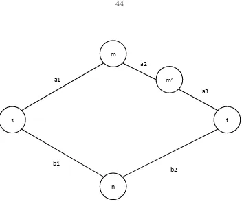
s
m
t
n
a1 a2
b1 b2
s
m
t
n a1
a2
b1
b2 m’
a3
Figure 3.3: The effect of adding a serial link
For this new network the set of paths is R = {r1, r2} with r1 = (a1, a2, a3) and
r2 = (b1, b2). and the demand function for path r1 is given by:
da1(p) =P(θr1 −pa1 −pa2 −pa3 +a1 > θr2 −pb1 −pb2 +b1),
with θr1 =θa1 +θa2+θa3 and θr2 =θb1 +θb2.
Then applying Proposition 9 it follows that an OE satisfies
The main effect of adding the linka3 is captured byθr1. In particular, forθa3 >0
the new link a3 affect the demand da1(p).
3.4.2
Merging analysis
In this section we show how our demand model can be useful to analyze merging de-cisions between two firms producing complementary goods. In terms of a networked market, we analyze the effect on equilibrium prices when two firms within the same path (bundle) decide to merge.
Formally, we are analyze the market with the structure displayed in Figure 3.4. In particular, we can think of firm a as the producer the main good, whereas firm
b1 and b2 are the complement ors to this main good. This simple directed network
captures the situation when consumers first need to buy the main good, and then they can enjoy the complements (b1 or b2).
An example of a real world situation that is captured by Figure 3.4 is the case where the main producer isM icrosof t, andb1 and b2 are two complementors to the
main good produced byMicrosoft. Concretely,b1 andb2 can be the complements for
Microsoft Windows. Our goal is to analyze the effect of merging firm a with firm b1
on the equilibrium prices.
From Proposition 3, we know the equilibrium prices for firm a and b1 takes the
form:
pOEa =ca+µa(pOE) and pOEb1 =cb1 +µb1(p
OE),
whereµa(pOE) = Fa(θa−pOEa +ϕ(p OE))
fa(θa−pOEa +ϕ(pOE)), µb1
(pOE) = Fb1(θb1−θb2−p OE b1 +pOEb2 )
fb1(θb1−pOEb1 +p OE b2 )
s t
m
b1
b2 O: Do not buy.
a
ϕ(pOE) =
E(max{θb1−p
OE
b1 +εb1, θb2−p
OE
b2 +εb2}).
Now let us suppose that firmaandb1merge, i.e., they maximize their joint profit
coordinating their pricing decisions. The equilibrium prices after merging are given by:
pOEa1 =ca+µa(p
OE) and pOE b1 =cb1.
The important property of the equilibrium prices after merging is the optimal price for firmb1 is to set price equal to marginal cost. The intuition for this result is
that once firma and b1 coordinate their pricing decisions, they internalize the effect
on being in the same bundle (path).
Chapter 4
Price competition, free entry, and
welfare in congested markets
4.1
Introduction
In many environments, such as communication networks in which network flows are allocated, or transportation networks in which traffic is directed through the un-derlying road architecture, congestion plays an important role in terms of efficiency. In fact, over the last decade the phenomenon of congestion in traffic networks has re-ceived attention in a number of in different disciplines: economics, computer science, and operations research.
marginal cost pricing. Under this mechanism users pay for the negative externality that they impose on everybody else.
Concretely, under a Pigouvian tax scheme users face two sources of cost: one due to the congestion cost and the second due to the toll. Nonetheless, Pigou’s solution is hard to implement in practice, because it requires that the social planner charges the tolls in a centralized way, which from a practical and computational perspective is a very complex task. Thus, the natural alternative is to consider a market based solution, where every route (or link) of the network is owned by independent firms who compete setting prices in order to maximize profits.1
Despite the relevance of and the increasing interest in implementing decentralized pricing mechanisms to reduce and control congestion in networks, little is known about the theoretical properties of such solutions. Indeed, little is known about the existence and uniqueness of equilibrium prices for general classes of network topologies.
In addition to the problem of the existence and uniqueness of a price equilibrium, a second problem that is raised in congested markets is the analysis of free entry and welfare. In particular, every firm can be viewed as a link, so the number of firms that enter the market will determine the network topology. Thus the socially optimal topology can be identified with the optimal number of firms in the market. Similarly to the study of existence and uniqueness of a price equilibrium, little is known about the free entry problem in general networks.
We point out that the analysis of existence, uniqueness and free entry in a network with multiple sources and a common sink is not only relevant from a theoretical perspective, but also from an applied point point of view. A real world situation
1For an early discussion of price mechanisms in congested networks, we refer the reader to Luski
where our model may be useful, is the case of the airline industry. In particular, we can think of in a situation where consumers from different locations (sources) want to travel to a common destination, let say d. Then consumers can choose among airlines (and combinations of them) to reachd, where the total cost faced by consumers is given by the price charged by airlines plus the waiting time (congestion). An understanding of the conditions when a unique price equilibrium exists and how free entry affects social welfare turns out to provide critical information for policy makers regulating this industry.
A second example where a general network analysis is useful, is the case of combi-natorial markets. In particular, in a large combicombi-natorial market, such as the Internet, the firms own links and set prices in order to maximize profits whereas consumers purchase bundles of products in order to maximize their utility. Concretely, we can consider the situation where each consumer is interested in buying bandwidth along a path from its source (origin) to its destination, and obtains a value per unit of flow that it can send along this path. In this environment, the analysis of the existence and uniqueness of a price equilibrium provides us information concerning how prices can be used to organize the market. For instance the understanding of the existence of price equilibria may be useful in the analysis of the efficiency of these markets.2
4.1.1
Our contribution
In this chapter we develop and study a general oligopoly model in a network subject to congestion effects. Our contribution is threefold. First, we introduce an alterna-tive notion of equilibrium in traffic networks, which we denote asMarkovian traffic equilibrium. Our equilibrium concept is based on the idea that users choose their
2For an analysis of the efficiency of combinatorial markets we refer to Chawla and Roughgarden
optimal paths in a recursive way. The idea that users can find their optimal paths in a recursive way turns out to be different to the standard notion of Wardrop equi-libria. We are not aware of previous papers studying price competition in congested markets using the notion of Markovian traffic equilibrium.
Second, we show the existence and uniqueness of a pure strategy price equilib-rium. Our result is very general: we do not assume that demand functions are concave nor impose particular functional forms for the latency functions (congestion costs) as is commonly assumed in the extant literature. We deriveexplicit conditions to guarantee existence and uniqueness of equilibria. We stress that our existence and uniqueness result does not rely on a specific network topology. In fact, our re-sult applies to any directed network with multiple origins and a common destination node.
Our third contribution is the study of entry decisions and welfare in congested markets. We show that the number of firms that enter the network exceeds the social optimum. In terms of network design the excess entry result means that the observed topology will not be the socially optimal. Because we obtain this result for a general network, we think of that our excess entry result may be useful in studying problems of optimal design of networks.
Markovian model is based onrandom utility models anddynamic programming. The use of random utility models allows for heterogeneity in users’ behavior, i.e., instead of assuming homogenous users, we model the utility of choosing a certain route as a random variable. In addition, and considering the stochastic structure of users’ utilities, we assume that users solve a dynamic programming problem in order to construct the optimal path in a recursive way. Thus, at each node users consider the utility derived from the available links plus the continuation values associated to each link.
Furthermore, the introduction of random utility models has the advantage of generating a demand system, which shows how prices and congestion externalities induce users’ choices.3
Combining the previous elements, we solve a complete information two stage game, which can be described as follows: In the first stage, firms owning the links maximize profits setting competitive prices a l`a Bertrand. In the second stage, given firms’ prices, users choose routes in order to maximize their utility, namely the cheapest route. We solve this game using backward induction, looking for a pure strategy sub-game perfect Nash equilibrium, which we call theOligopoly price equilibrium.
Related Work: The pricing game that we study in this chapter is not new at all. In
fact, this class of games is studied in Cachon and Harker [2002], Engel et al. [2004], Hayrapetyan et al. [2005], Acemoglu and Ozdaglar [2007], Baake and Mitusch [2007], Allon and Federgruen [2007], Allon and Federgruen [2008], Chawla and
Roughgar-3We stress that our approach differs with the one known as aggregation in oligopoly markets
den [2008], and Weintraub et al. [2010]. In order to establish the existence of an oligopoly price equilibrium, these papers assume the following: First, in order to describe users’ behavior these papers make use of the concept ofWardrop equilibria, which establishes that utilities (costs) on all the routes actually used are equal, and greater (less) than those which would be experienced by a single user on any unused route. Second, these papers impose assumptions on the demand generated by users’ behavior or assumptions on the class of latency functions. In particular, Cachon and Harker [2002], Engel et al. [2004], Hayrapetyan et al. [2005], and Weintraub et al. [2010] assume that the demand functions are concave (or log-concave) functions of the price charged by firms. Thanks to the concavity assumption, the previous pa-pers show the existence of an oligopoly price equilibrium. On the other hand, the papers of Acemoglu and Ozdaglar [2007], Baake and Mitusch [2007], and Chawla and Roughgarden [2008] show the existence of a pure strategy equilibrium assuming that the latency functions are affine.
Moreover, all of the papers mentioned above, consider a simple network consisting of a single origin-destination pair, with a collection of parallel links. This specific network topology rules out some interesting examples from an applied point of view,4
thus limiting the application of the available existence results.
The recent papers of Allon and Federgruen [2007, 2008], use random utility models to study price in competition in the context of queuing games, where the latency functions represent the waiting time that users must wait to be served. These papers establish the existence and uniqueness of an oligopoly equilibrium. However, the results in Allon and Federgruen [2007, 2008] differ from ours in two important aspects. First, Allon and Federgruen [2007, 2008] consider a network consisting of a single origin-destination pair with parallel links, thus ruling out important cases from an
applied perspective. Second, Allon and Federgruen [2007, 2008] do not study the entry and welfare problem.
Regarding our result on free entry and welfare, similar findings in the context of traditional oligopoly theory can be found in Mankiw and Whinston [1986] and Anderson et al. [1995]. These papers do not, however, deal with network structures on congestion; features that are crucial components of our result. For the case of congested networks, a similar result to ours can be found in the recent paper of Weintraub et al. [2010] for the particular case of a network with a single pair source-sink and assuming parallel links. Summarizing, our results can be viewed as a generalization of previous findings of the free entry and welfare problem.
The rest of the chapter is organized as follows: Section 4.2 presents the model. Section 4.3 studies the free entry and welfare problem. Section 4.4 shows the exis-tence and uniqueness of a oligopoly price equilibrium for a general class of latency functions. Finally, Section 4.5 concludes. Proofs and technical lemmas are presented in Appendix C.1.
4.2
The Model
Let G = (N, A) be an acyclic directed graph representing a traffic network, with
N being the set of nodes and A the set of links respectively. Let d ∈ N be the destination node (or sink). For each nodei6=d,gi ≥0 denotes the numbers of users
starting at that node. We interpret gi as a continuum of users. For all i 6= d, we
denoteRi as the set of available routes connecting nodei with the destination node
d. Every linka is represented by a convex and strictly increasing continuous latency functionla:R7→(0,∞), which we assume to be twice continuously differentiable.
of users using linka. Any flow vectorv must satisfy the flow conservation constraint:
gi+
X
a∈A−i
va=
X
a∈A+i
va, ∀i6=d, (4.1)
where A−i denotes the set of links ending at node i, and A+i denotes the set of links starting at nodei. The set of feasible flows is denoted by V.
We introduce firms into the network through the assumption that each link a
is operated by a different firm that sets prices in order to maximize profits. In particular, firm a’s profits are given by:
πa(p, va) = pava ∀a∈A. (4.2)
Profit maximization generates a nonnegative price vectorp, p= (pa)a∈A.
In addition, and without loss of generality, we set the parameterR >0 to be the users’ reservation utility at each link a. Thus, given a flow v and a price vector p, the users’ utility is given by:
ua=R−pa−la(va), ∀a∈A.
We look for an Oligopoly price equilibrium using backward induction, i.e., given a price vector p, we solve the users’ problem. Given the optimal solution for users, we solve the firms’ problem.
It is worth noting that the previous framework is deterministic, so the notion of Wardrop equilibria turns out to be suited for solving the users’ problem. Thus the firms’ maximization profit considers the demand generated by this solution concept. This way of analysis has been traditional in the context of pricing in congested markets, and examples of its use are the papers of Acemoglu and Ozdaglar [2007], Engel et al. [2004], Hayrapetyan et al. [2005], Weintraub et al. [2010], and Anselmi et al. [Forthcoming].
In this chapter we propose an alternative model to study pricing in congested networks. In particular, we consider heterogenous consumers, where one of the main features of our approach is that the users’ optimal solution is based on the combina-tion of random utility models and dynamic programming. The next seccombina-tion describes in detail these ideas.
4.2.1
Markovian traffic equilibrium
In this section we introduce our equilibrium concept for the users’ problem, which is based on two important features. First, to solve the users’ problem we introduce the idea of random utility, which takes into account the heterogeneity of users’ prefer-ences. Second, we use techniques borrowed from dynamic programming to find in a sequential way the optimal path for users. We now proceed to explain in detail our approach.
According to this, the random utility uea may be defined as
e
ua =ua+a ∀a∈A,
with {a}a∈A being a collection of absolutely continuous random variables with E(a) = 0 for all a. At least two justifications for introducing {a}a∈A can be given.
The first explanation comes from the fact that at each link a, the random variable
a takes into account the variability of users’ reservation utility. This means that
at each link a we can model the reservation utility as a random variable defined as
Ra =R+a, with E(Ra) =R. A similar justification can be given if we model the
congestion costs as random variables. Concretely, for any given flow vector v, at each link a we can consider the random cost defined as ela(va) = la(va) +a, where
E(ela(va)) =la(va). 5 For all i6=d, let Ri denote the set of routes connecting nodei with destination d. Thus, for a route r ∈ Ri, we define its utility as ˜ur =Pa∈ru˜a,
and therefore the optimal utility ˜τi = maxr∈Riu˜r as well as the utility zea =eua+eτja can be rewritten as ˜τi =τi+θi and ˜za = za+a, where ja denotes that node j has
been reached using the link a, and E(θi) = E(a) = 0. Each user traveling towards
the final node, and reaching the node i, observes the realization of the variables ˜za
and then chooses the link a ∈A+i with the highest utility. This process is repeated in each subsequent node giving rise a recursive discrete choice model, where the expected flowxi entering node i6=d splits among the arcs a∈A+i according to
va =xiP(eza ≥ezb, ∀b∈A
+
i ). (4.3)
5We can also consider the case where the utilities of every link are deterministic and the
Furthermore, the recursive discrete choice model generates the following conservation flow equations
xi =gi+
X
a∈A−i
va. (4.4)
Using a well known result in discrete choice theory (see Anderson et al. [1992]), equations (4.3)-(4.4) may be expressed in terms of the gradient of the functionϕi(·)
defined asϕi(z)≡E(maxa∈A+i {za+a}).6 In particular, the conservation flow
equa-tions (4.3) and (4.4) may be rewritten as
va=xi∂ϕi∂za(z) ∀a∈A+i ,
xi =gi+Pa∈A−i va,
(4.5)
where ∂ϕi∂za(z) = P(zea ≥ezb, ∀b∈A
+ i ).
Given the recursive structure of the problem, we may write the corresponding Bellman’s equation in the form τei = maxa∈A+i zea using zea = uea+τeja. Thus, taking expectation we get
za=ua+ϕja(z) (4.6)
or in terms of the variables τi
τi =ϕi (ua+τja)a∈A
(4.7)
In order to simplify our analysis, we assume the following two conditions for the
random variables {a}a∈A.
6The functionsϕi(
programming problem. This means that instead of choosing routes, users recursively choose links considering the utilities and the continuation values at every node. The method of solving recursively the users’ problem turns out to be completely different from the standard notion of Wardrop equilibrium.8 We shall call this solution concept
Markovian traffic equilibrium. Its formal definition is:
Definition 6 Let p≥ 0 be a