2D Upper Body Pose Estimation from Monocular Images

2D Upper Body Pose Estimation

from Monocular Images

Jeroen Broekhuijsen

Master’s Thesis Computer Science

Human Media Interaction Group University of Twente

Enschede, March 2006

Abstract

This research describes how 2D upper body pose can be estimated from the

monocular images of recorded meetings. These recorded meetings are provided by the AMI project which develops new technologies for interaction between a computer and human beings in technology-mediated meetings.

This work can be used to automatically annotate videos. The poser can be further researched for an improved understanding of actions during meetings. In the video data from these meetings there are two people present which usually face the camera. There is no calibration data or body size information available. To estimate the pose of the upper body this research first looks at which features are available in

comparable research, next potential image features are discussed and then the features that are usable in the AMI data are discussed, which in this case are the silhouette, skin area and edges.

The silhouette is calculated using background subtraction, the skin color area using HSV color space thresholding and the edges using a combination of Sobel kernels. Erosion and dilation are used for noise removal.

The pose is estimated comparing the silhouette to shoulder templates, tracking the skin color blobs for the head and hands and use an edge histogram to determine the most likely location for the elbow. The combination of the results from these features leads to a 2D model of the upper body. The results from the current frame provide the initialization data for the next frame.

Acknowledgements

Table of Contents

1. Introduction...4

1.1 Goal...5

1.2 Context...5

2. Related work ...8

2.1 Introduction to Posture Estimation ...8

2.2 Features in related work...12

2.2.1 Silhouette ...12

2.2.2 Color & Texture...14

2.2.3 Edges...18

2.2.4 Motion...20

2.3 Conclusion ...21

3. Analysis of Features...22

3.1 Silhouettes...22

3.2 Color & Texture...23

3.3 Edges...23

3.4 Motion...24

3.5 Conclusion ...26

4. Design of the pose estimation system...27

4.1 Setup ...27

4.2 Processing ...29

4.2.1 Silhouette ...29

4.2.2 Skin color...30

4.2.3 Head & Shoulder Locator ...31

4.2.4 Elbow Locator...34

4.2.5 Head & Hand Locator...40

4.2.6 Combine results ...42

4.2.7 Provide Feedback...43

4.3 Conclusion ...43

5. Evaluation of algorithms...44

5.1 Shoulder detector ...45

5.2 Head & Hand finder...50

5.3 Edge limb finder ...53

5.4 Evaluation ...55

6. Conclusion ...61

1. Introduction

In science fiction computers have always been able to distinguish the people in their surroundings. If it were possible now, it could lead to various new ways to interact with the computer, but letting computers interact with human beings has always been difficult. The first interaction between humans and computers started with punch-through cards, later keyboards and mouse were used and nowadays it is even possible to use voice-commands. In the future it could be even better, when a computer could see the user when he makes a certain gesture, it could know what the users means and interpret this as a command, as can be seen from various movies nowadays. This new way of interaction with a computer could also lead to various other purposes:

providing new ways of automatic surveillance, making surveillance more robust and autonomous, using your body to control a virtual body on the PC or be able to recognize and react on your emotions. However, before this is possible the computer would first have to be taught to see and recognize the user.

Currently, the best way for a computer to see a person is a motion capture system. Motion capture systems are used to capture the pose and motion of the body and the recorded data can be used to make computer generated graphics in films and games look more authentic or can be analyzed to aid and improve the performance of for example athletes.

In motion capture multiple cameras are used to record the user in a specific room where the user is wearing a special suit that has special markers for example special colored stickers. The motion, the way the body moves, and posture, the way the body is positioned, can be captured by keeping track of these markers.

These studios are very costly and rely on these special conditions, markers and careful initialization to determine the posture of the person in the video, as can bee seen from figure 1 below.

done in recent years to determine the motion and posture without these markers and using cheaper equipment.

Estimating posture without markers is a lot more difficult. The computer no longer has pre-set markers to find the body coordinates and needs to look for other marks in the image. However, these marks are no longer something that is well known, such as the special colored dots in figure 1, but have become the specific characteristics of the person in the image. The characteristics of the person in the image are the features with which the person can be recognized. Instead of these features being always the same in the motion capture studio, now these features vary with each person’s appearance, situation and environment. The computer needs to learn to see the body, using these features from the images.

The European AMI project [AMI] tries to develop new technologies for multi-modal interaction between the computer and a human being. Multi-modal, or multiple modalities, can be interpreted as interaction using: speech, vision, tactile information, etc. The context of this interaction is (smart) meeting rooms.

This research will contribute to this project by annotating data from the AMI project in which scripted meetings have been recorded by video cameras and can be

processed to generate a virtual body representation. The resulting posture can then be analyzed to look for gestures, actions, behavior and emotion to further develop multi-modal interaction.

Section 1.1 will set the goal of this research and section 1.2 will set the limitations and domain for this research. Chapter 2 provides a further introduction to estimating posture and describes how previous research has used features to estimate posture.

1.1 Goal

The goal of this research is:

To estimate the 2D upper body posture of a person in the AMI video data.

In order to reach this goal this research first has to describe what posture is and how posture is generally estimated. Which features exist and whether they can be applied to the AMI video data [AMI2] and look at how the information from these features can be translated to an upper body posture. Finally several test videos are manually annotated in order to evaluate the performance of the developed system when these videos are automatically annotated by the posture estimation system.

1.2 Context

The context in which the posture is estimated limits the amount of methods that are usable and sets the constraints on the posture estimation system. Only few methods are applicable outside the context they were initially developed in.

mainly on the domain set by the AMI project. An example of images from a meeting can be found in figure 2.

Figure 2: Two examples of input images from the AMI project.

In the AMI project there are several advantages similar to the advantages present in motion capture systems, but also several disadvantages which make estimating posture more difficult. Moeslund has written a survey on posture estimation in the past few years and defined two categories for the assumptions that can be made: movement and appearance assumptions [MOES].

These assumptions can also be applied to the AMI data and can make the problem easier by setting constraints and limitations to the possibilities that could occur in the image or can make the problem more difficult by increasing ambiguity and

uncertainty to the information in the image.

Assumptions based on appearance that make it easier:

• The workspace is indoors, has constant lighting and a static background • The people in the image almost always face the camera

Assumptions based on appearance that make it more difficult:

• There is no calibration data available on the cameras or a prior model of the subjects in the video data

• Clothing of the subjects varies and only their upper body is visible • There are always two people present in the images

• Only one input camera is used

Assumptions based on motion that make it easier: • The cameras are stationary

• The people in the image move slowly

Assumptions based on motion that make it more difficult:

In the survey, Moeslund also describes how the posture estimation process can be divided in four steps:

• Initialization:

the model has to be manually or automatically initialized to provide a starting point for the algorithms

• Tracking:

posture data is tracked along each subsequent frame to update the areas of the model instead of reinitializing the data each frame • Pose Estimation:

data gathered by special filters and algorithms is used to estimate the posture in an image

• Recognition:

the sequence of estimated

postures can be used to recognize actions

Figure 3: [MOES] Four steps of posture estimation. Yellow: The area of this research. Green: The focus of this research.

Since the goal of this research is to estimate the 2D upper body posture in the AMI data, this research will not look into the recognition step of posture estimation. It will only handle the initialization, tracking and pose estimation steps, where the focus of this research will be on the pose estimation step.

Chapter 2 will provide an introduction to posture estimation and discuss common features. Chapter 3 will explain if the features are applicable inside the AMI domain. The 4th chapter will propose a pose estimation system and explain how the features are used. In chapter 5 the results from this system will be shown which will be discussed in chapter 6.

Initialisation

Tracking

2. Related work

Since computing power has dramatically increased in recent years so has the capacity to determine the motion and posture of a human being. However, with the current level of technology the solution of always finding the correct posture is still far away. But, by limiting the context it is no longer necessary to always find the correct

solution for every situation. By applying constraints on the domain there are fewer possible situations and it is easier to find a correct solution. Currently researchers have tried to estimate posture by looking at specific features within a limited domain.

First section 2.1 will further introduce what posture estimation is and how it is usually estimated. Next, section 2.2 will discuss how researchers have used the most common features to estimate the posture in their specific domain. Finally, section 2.3 will discuss which possibilities could work in the domain of the AMI data.

2.1 Introduction to Posture Estimation

Before posture can be estimated it is necessary to first determine what a posture actually is, then how we can represent this posture and last how the computer can find the posture in an image.

Posture

Posture can be defined as the arrangement of the body and its limbs. When posture within an image is estimated the current arrangement of the body in a particular image has to be found. There is a mapping of the person’s body in the input image to a body model. An example of this mapping can be seen in figure 4 where all joint locations were manually defined and the 3D body model generated according to these locations in the image using a body model.

Body Model

To help the computer represent the body it can use a model. Gavrila has written a survey describing the various types of body models in posture estimation of the last few years [GAVR] and distinguishes three body models.

• No body model, the posture is found in terms of low level features. These low level features are used to train a system that statistically matches these features with a posture, see figure 5 left.

• 2D body model, the model provides information on the 2D view of the body, see figure 5 middle.

• 3D body model, the model provides information on the 3D view of the body, see figure 5 right.

Figure 5: Left: example of components that lead to a posture without using a body model, these low level features are the result of using training data to train wavelet templates [OREN]. Middle: example of a 2D body model [LEUN]. Right: example of a 3D body model [GAVR2]

A body model also includes kinematic information, which is the way the limbs are connected and how they are able to move and occlude each other. This provides a helpful limitation to the movements the body can make.

The model can be used not only to represent the found data, but also to help during the posture estimation process itself since more information on the appearance and kinematic connections of the person is available.

In Moeslunds survey this process is described as analysis by synthesis. First, the new body position is predicted, then the model and image are matched and finally the model is updated according to the results from the matching process.

Issues when finding posture

Figure 6: Examples of different appearances due to clothing [ZHAO].

Figure 7: Examples of different appearances due to posture [ZHAO].

Figure 8: Example of the use of more than one camera [MIKI].

Figure 9: Example of the different appearance of people in the natural environment or inside a well defined room [ZHAO] [UEDA].

Some examples of how a person can appear in different situations are displayed in figure 6, 7, 8 and 9. Occlusion occurs in figure 6, 7 and 9 where not all body parts of the person are visible. In figure 6 and figure 7 the persons in the image wear different clothing creating a different appearance. Sometimes multiple cameras are used to handle occlusion where not all body parts are visible, see figure 8 and figure 9, but this is not possible in all situations.

Most solutions only work inside their well defined domain and are not usable for other situations. A stable indoors situation requires less robust methods compared to a changing outdoor situation. The appearance of the person in an image also requires different methods, for example when the clothing is tight, loose, colored, textured or uniform. A robust solution that covers all areas has not yet been found. This research will not try to come to a robust solution in all situations since its main focus is the indoors situation of the AMI project. It will however try to be as robust as possible in the AMI context.

Features

The characteristics of the person in the image are the features with which the person can be recognized. From figure 6, 7, 8 and 9 can be seen that in each situation the characteristics of the person are different. This also means that in each domain the features that can be used to find these characteristics will be different.

Posture estimation

Since posture, body model and features have been introduced the estimation process itself can be explained in more detail. Following the classification done by Moeslund the general layout of a posture estimation system without recognition is described by figure 3. This general layout however does not explain what happens to the image and how the posture is estimated.

A more detailed view of these four steps appears in figure 10 and 11 which describe the posture estimation system of this research. The initialization phase is optional and is drawn with a dashed line. Both the tracking and initialization phase can also be integrated inside the algorithm within the pose estimation part. Initialization is drawn outside the pose estimation part to provide a better overview, tracking can be done for the whole body model, and for the internal values of an algorithm.

Figure 10: Example of a pose estimation system. The four steps described by Moeslund are also present. The initialization step is dashed since it is optional and only used in the first iteration.

As can be seen from figure 10, the pose estimation step first applies one or more feature finders on the input image and then uses an algorithm that combines the results from these features and estimates the posture which can then be used for the recognition step.

Increasing robustness

Some researchers have used only a single feature, such as silhouette, motion, and color or edge information to find all the body parts. They however rely on this single feature in which all body parts are easily distinguishable. If one of the body parts is no longer distinguishable by this feature, other information is required to find it.

A recent trend that provides extra robustness for posture estimation is to look for individual body parts, instead of using one, or the same, algorithm for the entire body as a whole [BLACK] [LEE] [NAVA].

The research done by [ZHAO] and [SENI] combines two methods to provide extra information. First the body is detected using silhouette decomposition, and then body parts can be aligned using edge information. The approach by Lee goes a step further because different methods are used for several body parts [LEE]. This is a similar approach compared to the work of Black where each body part has its own detector

Pose Estimation

Input image Output

If this is applied to the schedule in figure 10, each body part finding algorithm would have its own set of features that are combined to estimate the location of the

individual body part, after which the results from these algorithms can be combined into one model, leading to figure 11. A more detailed description of the individual parts will follow in chapter 4.

Figure 11: Example of a pose estimation system with separate detectors. The four steps described by Moeslund are also present. The initialization step is dashed since it is only used in the first iteration.

2.2 Features in related work

Whether simple or robust, features are the key elements that all algorithms rely on. The features themselves need to be explained before a method can be discussed that determines how bodies and algorithms can be combined. This research cannot go into detail of all available features, but will look into the most commonly used features available.

The features this research will cover are:

• Silhouette • Color & Texture

• Edges

• Motion

The next sections will briefly discuss these features which have been used by researchers to estimate posture from an image. Chapter three will discuss whether these mentioned features are applicable in the AMI domain.

2.2.1 Silhouette

The silhouette is the contour of an object. It provides information where the object is located, what shape it has and which pixels in the image belong to the object.

Piccardi has written a review of various methods of background subtraction to find the silhouette [PICC]. The easiest method is the direct subtraction of a background

Pose Estimation

Input image Calculate

good silhouette. A different method, subtraction of a median, running average or Gaussian mixture would be better to adjust to a new situation if any changes occur.

Other ways of finding the silhouette can be to segment the image using colors or texture which is explained in more detail in section 2.2.2. Multiple cameras can also be used to create a foreground / background model based on a depth map of stereo images, see figure 12. Another method to find the silhouette is motion, see section 2.2.4.

Figure 12: Left: original input image from the left view. Middle: original input image from the right view. Right: depth image from the combination of stereo images which is used to generate a silhouette [GEL].

Silhouette & posture estimation

Several researchers have tried to decompose the silhouette in body parts and use this input to calculate the estimated pose [ZHAO][SAPP][TAKA], see figure 13, 14 and 15. Lee and Cohen use template matching to find the head and shoulders in the silhouette [LEE], see figure 16. Lee also uses another method to find the posture by aligning a template with the detected silhouette [LEE2]. Poppe and Lee use a method to verify that the generated posture silhouette overlaps or matches with the silhouette from the input image. This is then used to verify if an estimated posture is viable or not, see figure 17 and 18 [POPP] [LEE2].

Examples from the described literature

Figure 13: [ZHAO] Using silhouette for posture estimation: First the silhouette is decomposed into limbs, then the 2d model is introduced with the known limb positions, lastly the limb positions are adjusted using edges.

Figure 15: [TAKA] Feature extraction from

silhouette using distance measures. Figure 16, [LEE], left: original input image, right: detected contour and shoulder points are displayed.

Figure 17, [POPP] Silhouette Verification, Left: Original Silhouette, Middle: generated silhouette from posture, Right: overlap between generated posture and original silhouette.

Figure 18, [LEE2] Silhouette Verification, Left: generated posture over original silhouette, Right: verification and fitting process.

2.2.2 Color & Texture

Color

Color & pose estimation

Color segmentation can also be used to create a model of the body using color blobs. Each blob can then be tracked and updated according to the new frame information, see for example the research done by [HEI] in figure 20. Wren has created a system where the head and hand blobs are tracked throughout the video using colored blobs [WREN]. These blobs are formulated using both spatial information and color information using histograms. Pixels from the image are allocated to the corresponding foreground blobs or background blob based on the Mahalanobis distance to each blob, see figure 21.

Example images from the described literature

Figure 20: [HEI] Left: starting image of a color tracker. Middle: tracking result of the first and last color images. Right: ending image of a color tracker.

Figure 21: [WREN] Left: original input image. Middle: color segmentation into blobs. Right: 3D-blob representation of the person.

Texture

Color can also be used to construct texture information from an image. Using these textures the image can be segmented into regions which have a similar texture. Gabor filters are usually used to construct textures [JAIN]. Another approach is to use the color histogram information similar to the work of Deng to construct textures [DENG].

Figure 23: [DENG] Left: original input image. Right: segmented image using color and texture information.

Texture & pose estimation

The methods mentioned above could also be used to calculate the silhouette of an object. Usually they methods are either too general, or too detailed. In the case of the tank in figure 22, the information is too coarse, whereas the image with the flowers in figure 23 is too detailed and the flower area is broken up into areas that are too small.

Ramanan created and uses a texture database with which body parts can be located [RAM]. Either a general texture database can be used to recognize general people, or a database can be created from a specific person to better recognize that person. These databases can be automatically filled without prior knowledge of the scene, see figure 24.

A model of a body can be constructed including a texture. This model can be used to verify the pose of the person in the image or align the body model to the actual image, see figure 25 [GREE]. Texture could also be used to find body parts if a texture model of the person is created [RAM].

Example images from the described literature

Figure 25: [GREEN] Left: original input image. Middle: textured model is overlaid on the input image. Right: expected result value after computation.

Skin Color

Research has shown that skin color is a very specific range in color space that can be used to look for non-clothed body parts such as a head, hand or arm. Even though the color of human skin does not vary much, there are a lot of other objects that are also skin colored, like for example cardboard. A skin color detector can provide a rough estimate of the location of body parts, but it also provides a rough estimate of non-body objects that are skin colored.

Skin color can only be found if the lighting and brightness conditions of the video are fairly constant. Vezhnevets has written a review of various skin color detection methods [VEZH]. Conversion to a color space and then thresholding the image is one of the most common methods to detect skin color. Other methods train a system with skin color pixels and use update methods to add new skin samples when new people appear.

Skin Color & pose estimation

Example images from the described literature

Figure 26: [ARGY] Using skin detection to

detect head and hands. Figure 27: [LEE2] Skin color detection to find head and hand coordinates.

2.2.3 Edges

An edge is the difference in contrast between several neighboring pixels in an image. Usually a Sobel filter, a convolution kernel as shown in figure 29 or 31, is used to calculate the edge value of each pixel in an image. At each pixel in the image the sum of the multiplication of the kernel with the input image is calculated. The kernel is centered at the current location in the image and is shifted so that it calculates this sum for each pixel in the image creating a map of edge contrast in an image. After all pixels are calculated this can be visualized by normalizing the edge values to

grayscale values and displaying them in an image. Figures 28 and 30 have examples of the resulting edge image using various methods. As can be seen from these figures the edges are usually present where a limb is present and can provide useful data for posture estimation.

Figure 30: Left: edge image using Laplacian kernel. Right: edge image using Canny edge filter. The canny edge filter first uses a blurring kernel, see figure

31 and then the Sobel kernel, see figure 29.

Figure 31: left: Laplacian kernel. Right: Gaussian blur kernel.

Edges & pose estimation

Researchers have used edges in every area of the posture estimation process. Most often it is used to align a template or model to an edge. Zhao uses the edges to align limbs to edges present in the silhouette, see figure 32 [ZHAO]. Dimitrijevic uses the edges to search for the silhouette using templates [DIMI], see figure 33.

Sidenbladh has trained a limb-finder that uses histograms of the edge values to determine if an edge belongs to a limb or belongs to the background, as can be seen from figure 34 [SIDE]. First a training set of images are pre-annotated and used to train a foreground/background histogram. Then the histogram is used to classify the chance that a predicted location corresponds to an actual limb, this method will be explained in more detail in chapter 4.2.4.

Example images from the described literature

Figure 32: [ZHAO] Left: detected contour. Middle left: the original estimated body poses. Middle right: the calculated edge image. Right: the adjusted body poses after edge matching.

Figure 34: [SIDE] Using an edge detector to train a limb detector (in this case lower arm).

2.2.4 Motion

Motion or more often called Optical Flow is the correspondence between small groups of pixels in two consecutive frames. Sometimes motion can provide extra information where other features provide no accurate data. Calculating motion however is very computationally intensive.

Motion & pose estimation

Since the body moves in certain patterns these patterns can be recognized and used for pose estimation. Ning has trained a motion model which he uses to calculate the posture information from an image [NING], see figure 36. He also uses motion to align the body model to the silhouette in the image.

Lee uses motion to track the limbs in the image. Figure 35 shows an example of the optical flow field that Lee and Cohen have used to calculate the direction of the flow and the after this is combined with several other viewpoint flow fields an estimate 3D direction is calculated and the body model moved accordingly.

Another way of using motion is to create a small template of for example a limb and search the new frame for this template, considering movement, rotation and

deformation. This however is also computationally very intensive. Sidenbladh used this method to train a limb finder using a histogram. A pre-annotated training set is used to calculate the movement at the limb edge locations. This histogram can then be used to determine the score for a new image and determine if it is more likely to be limb or background, the method is similar as described in the edges chapter [SIDE].

Figure 36: [NING] Using optical flow to align a body model with the actual image.

2.3 Conclusion

All the features used by the researchers from section 2.2 can lead to a body model from a monocular image. However, not all the algorithms used by these researchers will also provide a solution in the AMI context. For example, the AMI project data has monocular images and the approach by Green using stereo images to get the silhouette will not work in the AMI context. On the other hand, because the AMI project has a static background and stable lighting conditions, the methods described by Piccardi are very likely to produce good results in finding the silhouette, possibly even better than using color histograms, and definitely more likely than edge

templates or pre-set body texture templates and neither of these two templates are available in the AMI data.

To find the individual body parts we need ways to distinguish the body parts in the image. The silhouette could provide information on the individual body parts with its shape. Color could be an appropriate solution if we look at the research from Wren, but it only works if the person in the image is wearing only plain clothing where the clothing of each body part would have has its own color. The approach using skin color however almost always provides a good estimate for the head and hands. Finding the hands using other means such as texture again depends on the clothing of the person in the image.

Using optical flow to find the individual body parts only provides information if there is prior knowledge available about the body. This means it is better used as a support feature than to actually find an individual body part from scratch. Edges are used similarly and are often used to align an already existing position to the image and almost never used to search for individual body parts. Using texture also only works after the body has been initialized.

Finding the silhouette and the head and hands are the most simple and most effective steps to find the upper body. Edges, motion and texture can provide additional information after the initial body has been placed at a reasonable position.

3. Analysis of Features

As section 1.3 discussed, not all features and algorithms provide a solution in a different context. The research discussed in section 2.3 provides a good solution to estimate the posture of a body from a monocular image, but does not necessarily lead to a good solution in the AMI context. This chapter will look at each feature in the AMI context and determine whether the feature is usable for the AMI project or not.

The features that will be reviewed are:

• Silhouettes • Color & Texture • Edges

• Motion

3.1 Silhouettes

The images from the AMI data are all indoors with almost constant lighting

conditions and background. These criteria make it easier to find the background in the image. More difficult is the fact that there are always two people present. This can create ambiguity due to occlusions.

Since the images are from an indoor environment, background subtraction can be kept simple. Subtraction of a pre-recorded background image can suffice. However, these background images will have to be created for each input video since lighting, color and background varies slightly in each video.

An example of a silhouette after background subtraction can be found in figure 37. The middle image shows the slight difference in brightness of the image. Even with this slight error background subtraction still produces an accurate silhouette. The silhouette from figure 37 also includes the paper and chair since they are not present in the background image. This could be a potential problem for later processing.

Figure 37: Left: original image. Middle: input background image. Right: extracted silhouette by background subtraction.

3.2 Color & Texture

Color

In the AMI data, see figure 38, there is no single solution to segment the color of the people to distinguish different body parts, as can be seen in the right picture.

Figure 38: Original input data, left and right images have different people and different clothing.

Texture

Since there is no prior body model or a texture model of the people in the AMI data, that can be used to determine where the person is. However, a texture model could be generated after a body model is established by the posture estimation process.

The clothing of the people however does not have enough difference in texture and color to be able to distinguish the different parts of the body.

Skin Color

Figure 38 shows it is better to segment the person into a clothed/non-clothed area than to try to distinguish the individual clothing areas. The non-clothed areas are the head and hands, which are skin colored. Since there is almost no difference in the

brightness conditions within one video and the people’s appearance always stays the same, color space thresholding provides an easy way to find the skin colored regions. This method does not take into account that the lighting is different in each video and the thresholds have to be manually adjusted for each different input video.

Figure 39: Example of skin color response generated from one of the AMI video streams. Left: original input image. Right: skin color result after noise removal and filling.

3.3 Edges

As can be seen from figures 40 and 41, limbs usually show up as edges, usually at the outer edge of the person, but also at the inner edges of the person. This can be

background and has large contrast differences on the edges where background and foreground meet. The edges inside the silhouette can be explained because of the way that clothing folds or because of shadows that are created by occlusion. These edges can provide useful data for posture estimation and can be used in various methods throughout the posture estimation system.

Figure 40: Left: original image. Right: edge image using Sobel kernel

Figure 41: Left: edge image using Laplacian kernel. Right: edge image using Canny edge filter.

3.4 Motion

Figure 42 shows the result of optical flow calculation in the AMI data using the Horn & Schunk [HOR] algorithm and when thresholded to show only the largest motion it has a lot of noise and does not always reveal clearly distinguishable movements of the limbs. Figure 43 shows a situation where movement is clearer in the images.

Figure 43: Left: original input image. Middle: calculated optical flow response frame. Right: calculated optical flow field. The size of the red and green lines indicates the amount of movement and the red half of the line indicates the direction of this movement.

The persons in the video do not move often. If there is movement it is usually too slow to be picked up correctly by the optical flow filter. The optical flow method shows better results when the timeframe between both input images is increased. When the optical flow vectors have been thresholded, distinctive movement can be seen in the body area. Even though the vectors have been thresholded, noise is still present in the background area, as can be seen from figure 43 right.

All optical flow images are calculated using the Horn & Schunk algorithm [HOR]. This method produces the least noise and best flow field compared to the Lucas & Canade approach [LUC]. Figure 44 illustrates the two approaches using the same settings. The middle image shows more responses at the actual locations where movement is present (the heads and the right arm of the left person). In addition, the approach by Horn & Schunk has less erroneous movement during non-moving sequences.

Figure 44: Left: original image. Middle: flow field using Horn & Schunk. Right: flow field using Lucas & Canade. The size of the red and green lines indicates the amount of movement and the red half of the line indicates the direction of this movement.

The persons in the video however rarely moves enough that any motion can be picked up. When the person in the image does move the calculated movement is not

3.5 Conclusion

Not all of the features discussed in section 3.1 till 3.4 provide enough information to find the body in the images from the AMI project. Section 3.1 shows that the

silhouette from the AMI video data does not have enough shape information to find all body locations of the upper body. The arms are not visible from the shape of the silhouette because they occlude the torso and because of the small distortions in the silhouette caused by the chair and paper. The head and shoulders however are very distinguishable. Using an algorithm based on the work done by Lee [LEE] the head and shoulders could be found.

Section 3.2 shows that skin color works really well in the AMI data to find the head and hands in the image, even though the entire lower arm will be found when people are wearing short sleeved clothing. The approach by Argyros [ARGY]could lead to good tracking of the head and hands and is very similar to the approach done by Lee [LEE].

Sections 3.2 till 3.4 show that texture, edges and motion only help when body parts are aligned with the data from these features. Motion has the least perspective for valid information. There is not enough consistent movement in the videos to provide supportive information for the body parts. Texture has a far better chance of providing supportive information but relies on the body already being found.

Edges on the other hand can provide a consistent and continuous source of information. The work done by Sidenbladh seems the most promising solution compared to the work of Zhao or Dimitrijevic.

4. Design of the pose estimation system

As stated in section 1.1, part of the goal of this research is to find a set of usable features in the AMI context which provide information to the estimate posture process. From chapter three we’ve seen that the silhouette, skin color and edge features are the most promising features in the AMI data, but it is not yet determined if these algorithms suggested in section 3.5 will also lead to posture estimation.

This chapter will discuss how the suggested features from chapter 3 can be used to find a pose. First, a more detailed setup of the pose estimation system based on these features and the layout from 2.1 will have to be introduced. Section 4.1 will discuss the setup of the system and section 4.2 will go into detail how each needed body part can be found using the features. Section 4.3 will discuss how these body parts are combined into the body model.

4.1 Setup

As can be seen from chapter 2.1, to increase robustness a system should not rely on only one feature or algorithm. Following Black, Lee and Navaratnam [BLACK] [LEE] [NAVA] it is better to look for individual body parts in the image and combine the results into one pose for the upper body of a human being. Each body part will need its own detection method(s) and the results need to be combined into a full upper body pose.

Figure 45: Two examples of input images from the AMI project.

From figure 45 can be seen that it is only possible to distinguish the upper body from the images. Since no information on the depth or camera calibration is available, the best choice for the body is a 2D model of the upper body, see figure 46. This model is a combination of a 2D joint location model and a 2D limb location model. The joint location model would include for example the location of the wrist and neck, but this model includes the location of the hand and face, since the wrist and neck locations cannot be found using the methods mentioned in section 3.5.

This model is expanded with the face area and the width of the arms. To fill this model the following locations will have to be found:

• Hand location, using skin color • Top of the Head, using the silhouette • Face location, using skin color • Width of the arms, using edges

Figure 46: Schematic of all locations that are used in the model of the body of this research, the outline is dashed since this model does not include the shape of the body, only the width of the arms is used.

Each body location can be tracked individually and initialized within the algorithm that finds it in each frame. The complete body model can also be tracked to provide feedback to the individual body location finders.

Figure 47: General layout of the pose estimation system, the initialization is done by the body location finders.

Figure 48: Detailed design for the pose estimation system. The additional feedback to the Combine

Top of the Head location

Shoulder joint

Finding Features Combine body

locations Input Video

Sequence Body location Finders

Not all of the connections have been included in figure 48 to simplify the figure. The initialization and trackers are also positioned inside the different body location finders and not displayed in the model of figure 49. The detailed description and connections of each component will be explained in the next section.

4.2 Processing

This section will explain each body location finder as shown in figure 48. Some body location finders require additional information from features to operate. Section 4.2.1 and 4.2.2 will discuss how these features are found, section 4.2.3 till 4.2.7 will discuss the other components from figure 48.

4.2.1 Silhouette

The silhouette can be used for almost all body part locators. It provides an easy way to limit the search area for body parts since body parts can only be present inside the silhouette area.

The silhouette does not provide much information on the layout of the body. The silhouette only provides a rough location of the total body. This limits the possibilities of how the silhouette can be used after it is found.

The arms are usually inside the torso area and not distinguishable from the silhouette. The only body parts that can be easily found are the head and the shoulders. However, if the arms would be above the shoulders the silhouette could no longer be accurate enough to provide a correct head location.

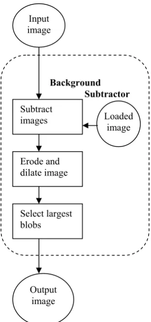
Section 3.1 explained that background subtraction is the easiest way to find the silhouette in the AMI data, figure 49 provides an overview of the process.

First a pre-made background image is loaded and subtracted from the input image. The resulting image is then thresholded to take into account small differences in lighting or color.

Figure 49: Design of the Background Subtractor that delivers the silhouette.

Then an erosion and dilation process is used to remove noise and background clutter, where erosion removes all image pixels which are not connected to a neighboring pixel and dilation draws all neighboring pixels for each pixel in the image. Lastly the largest blobs are selected and filled to remove other possible foreign

A B C D E Figure 50: A: input image. B: thresholded image after background subtraction. C: eroded image to remove noise. D: dilated image to strengthen the strong blobs. E: resulting image with largest blobs filled.

4.2.2 Skin color

Skin color only provides information on the skin colored objects in the image. This means it only provides information on the head and the hands, and sometimes arms if the clothing the person is wearing is short-sleeved.

First the input image is masked with the silhouette. Then the RGB input image is

transformed to HSV color space and thresholded using a threshold for the Hue and Saturation [POPP]. The HSV color space is less influenced by lighting changes. An erosion and dilation process is used to remove noise. They can be set according to the needs of each video. Lastly the largest skin colored blobs are filled and used to generate the output skin color image.

Figure 51 shows the process step by step and figure 52 shows the layout of the process as described above.

A B

C D E

Figure 51: A: original image. B: resulting skin color image.

C: eroded image. D: eroded and dilated image. E: resulting Figure 52: Design layout of the Skin Color Detector. Input

image

Skin Color

Detect skincolor

Erode and dilate

Select largest blobs

Output image

4.2.3 Head & Shoulder Locator

Sometimes additional objects such as the chair, papers or table make up parts of the silhouette. This can disrupt the process of finding the body parts. When the silhouette is combined with edge information more detail on the body parts is available, see figure 57. Similar to Lee [LEE] it should be possible to match a template with the silhouette and detect the head and shoulders. To this end 13

templates have been created which can be matched to the actual silhouette from an input image. For the other body parts, such as the arms, there is no information in the silhouette which can be used. Another method will be needed.

Following figure 55 the process can be explained as follows.

To find the head and shoulders, first the top area of each silhouette is taken, see figure 53. As noted in 4.2.1 this will no longer work if the arms are above the shoulders, but in the AMI data this does not occur.

Figure 53: Left: input silhouette. Right: top area of each silhouette.

If the detector has not yet been initialized it will first compare the top area silhouettes with several stored templates. The best matching template is then selected and snaked, an explanation of snakes can be found in the next section, to better resemble the actual silhouette from the image. This snaked version of the template is then stored internally and used as the template input for the next frame. When the stored template does not match the loaded template anymore the internal template is reset and re-calculated in the next frame to prevent drifting.

Figure 54: Design layout of the Shoulder Detector.

After the template is stored the body coordinates belonging to that template are loaded and adjusted by comparing the location in the template to the location in the silhouette from the image. The resulting coordinates are the output to the system and the

When the shoulder coordinates are above the template they have to be adjusted downwards, when they are below the template the difference between the input template and the loaded template can be calculated and is used to adjust the shoulder coordinates. Figure 55 C and D show an example of these coordinates.

A B C D

Figure 55: A: input silhouette. B: best matched input templates. C: similarity measure to actual silhouette. D: resulting head and shoulder coordinates.

The next section will first explain process of snaking an image and then the template matching process which are both used in the head & shoulder locator.

Snakes

The edge image is used to align the silhouette from the template to the actual position of the body using a snake [KASS]. The snake adjusts each pixel of the template to the edges in the edge image, see figure 56.

Figure 56: Left: original input template. Right: resulting silhouette after snaking with edge image.

The adjustment of the snake is based on minimizing the energy of the snake. The energy, Etot, depends on the internal and external energy. The external energy, Eext, is

provided by the image, see figure 57.The internal energy is based on the curvature and continuity energy. The curvature energy, Ecur, keeps the snake locally smooth. The

continuity energy, Econ, keeps the distance between the points on the snake the same.

For each point of the snake the surrounding pixels are checked to see if they provide a lower total energy for the snake.

This results in the following formula [KASS]:

ext cur

cont

tot

=

Ε

+

Ε

+

Ε

Ε

α

β

1

,

1

,

)

(

1

−

−

∀

=

−

=

Ε

v

v

d

i

n

2

+

−

v

v

In the formula vi is the ith point on the snake and dmean is the average distance between

the points on the snake. The factors α, β, γ are weighing factors which are set to 0.5, 1.0 and 1.0 based on several test runs.

Template Matching

First a template is loaded from file and placed at the correct silhouette location.

Then the edge information from the input image and the silhouette is combined to provide a way to align the template to the actual person using a snake. The absolute edges are calculated for the original input image and the silhouette image and both images are then added using a weighing factor of 0.3 and 0.7 for the silhouette edge image and the edges from the original input image. The resulting edge image looks as in figure 57. Several other weighing factors were tested to see how well the snaked version matches the actual body and the factors 0.3 and 0.7 provided the best results.

Figure 57: Left: original input image. Middle: silhouette image. Right: edge image combined by adding the original input edges with the silhouette edges.

The loaded template is then snaked with the edge image and the resulting contour is matched with the original loaded template. The original input silhouette is also snaked with the edge image and matched with the loaded silhouette. The resulting error rate from both matches are weighted and used to select the proper template.

The weighing method is: Error = 0.9*T1 + 0.1*T2

Where T1 is the snaked loaded template matched with the loaded template, and T2 is

the snaked silhouette matched with the loaded template. The template with the lowest error is the best match and is selected as the best candidate to continue. The weights of 0.9 and 0.1 are based on several test runs.

In this research three different types of matching have been tried and evaluated. The first method is the matching surface of two templates, which is the intersection area in percentage of the union area of both templates. The second method is calculating the Hu moments [HU] and calculating the sum of the differences between the logarithm of the Hu moments of both templates. The last method calculates a Pair-wise

Geometrical Histogram (PGH) [IIVA] for both templates and then compares both histograms with each other.

4.2.4 Elbow Locator

As could be seen from chapter 3.3 edges are usually present at the contour of the person, and inside the silhouette where occlusion occurs or shadow appears.

The elbow locator is based on the research done by Sidenbladh [SIDE] who uses the edges in the image to align the individual body parts, such as arms and legs.

The elbow locator only works when the shoulder and hand coordinates are known.

If the shoulder and hand locations are known it can search an area of the image to find a best solution for the elbow. When the elbow position from the last frame is also known the search area is limited to shorten calculation time. After the best location for the elbow is found the elbow locator calculates the thickness of the arms and the exact best location of the elbow. To evaluate all the positions in the image the elbow locator uses several histograms which are pre-trained using the training data supplied by Sidenbladh [SIDE02]

These histograms provide a scoring method to see if the score of a pixel is more likely to belong to the

background or to a limb. The input image is searched for the best location that could belong to the upper or lower arm. Or it can be used to verify or improve a coordinate already found for the arms. Figure 60 displays the above described process of finding the elbows.

The methods of how these histograms are created and how the score is calculated will be described in the next two sections.

Figure 58: Design layout of the limb finder.

Training Histograms

The histograms that are used in the scoring method are pre-trained using the training data from Sidenbladh [SIDH]. In this training data, several images are manually annotated with the edge locations of the upper arm, lower arm, torso, upper leg and lower leg. Since this research only focuses on the elbow location, only the upper and lower arm are used. To create the histograms, each image is converted to an edge image dependent on the current angle of the limb edge.

Figure 59: Left: original image. Right: resulting angle dependent edge image.

The edge image is constructed using Sidenbladh’s calculations for an angle dependent edge image. The angle of the limb determines the resulting edge response.

First the horizontal and vertical edge images are calculated. Then the horizontal and vertical components are multiplied with the sine and cosine components of the angle.

fe(x, θ) = sin (θ) fx(x) − cos (θ) fy(x)

Where fe(x,θ) is the resulting edge value of the pixel x at limb angle θ, fx(x) and fy(x)

are the horizontal and vertical edge components, see for several examples figure 59 and the top row of figure 60.

A histogram is created for each body part and for each body part the angle dependent edge image of the input image is calculated. For each histogram the manually

annotated locations of the body parts are sampled on the manually defined locations in the edge images and the distribution of values from the edge image on the location of the arm is calculated. These distributions of values are calculated for each limb in all the images and added together, creating a histogram where the y-axis is the amount of pixels found for a particular limb at a particular edge response which is the x-axis of the histogram.

A similar histogram is calculated for the background using several random locations taken from the background that have the same thickness and length but are calculated at varying angles.

By dividing these histograms with the total amount of samples taken they describe the chance that a certain edge value occurs on a manually marked location and the chance that it occurs in the background. Both histograms can then be divided by each other and the log of the resulting histogram shows an indication of an edge value belonging to the limb or background, given its parameters in the image.

Figure 60 shows three sample images from the Sidenbladh training data. In these three images the left lower arm of the person in the image is shown with the surrounding white box. The random locations for the background histogram are also shown in the image.

The histograms corresponding to the images are shown in the bottom row of figure 60. The histograms of the limb are the lower histograms, the histograms of the

background are the middle histograms and the division of both histograms is shown in the top histograms.

locations have almost no edge value, which is shown in the histogram where the edge values are almost all located in the centre, indicating no edge value. The second and third images show arm locations which are not as sharp in contrast and have a more spread edge value on the limb location and in the background. The resulting

histogram when all the histograms from all images are added together can be found in figure 61 and 62.

Figure 60: Top row: edge images from the Sidenbladh training data. Bottom Row: Corresponding edge histograms. The top histogram displays the spread of edge values in the background of the image. The middle histogram displays the spread of edge values of the lower arm in the image. The bottom histogram displays the log of the division of both histograms. The x-scale for the histograms is from edge value -128 to edge value 128 where the center edge value is zero. The y-scale indicates the occurrence of the value, where the top is no occurrence and the occurrence increases toward the bottom.

Figure 61: Top: background histogram of scores. Bottom: foreground histograms of edge scores. The x-scale for the histograms is from edge value -128 to edge value 128 where the center edge value is zero. The y-scale indicates the occurrence of the value, where the top is no occurrence and the occurrence increases toward the bottom.

Figure 62: Resulting scoring histogram The x-scale for the histograms is from edge value -128 to edge value 128 where the center edge value is zero. The y-scale indicates the chance of the value being on the limb, or in the background. where above zero is belonging to the limb, and below zero is belonging to the background.

The top-left histogram is the histogram created by the edge values in the background, the bottom-left histogram is created by the edge values on the limb locations. The right histogram is the division of both histograms.

As can be seen from the bottom-left histogram, statistically there are fewer pixels with an edge score of zero on a limb location. As can be seen from the top histogram the background has a lot more pixels that have an edge value of zero. This result is also visible if both histograms are divided by each other and thus show the similarity measure, see figure 62. If a pixel has no edge value, its score in the histograms is negative and more likely to belong to the background histogram, when a pixel has more edge value it is positive and more likely to belong to the limb edge histogram.

Scoring Method

These histograms provide a scoring method to see if a pixel is more likely to belong to the background or to a limb. The input image can be searched for the best location that could belong to the upper or lower arm. Or the histogram can be used to verify or improve an elbow location already found for the arms.

Each edge response value on a sample limb location gives an indication whether it belongs to the limb location, or to the background according to the trained histogram. All scores along the sample limb location can be added to provide a total score indicating the similarity of the entire limb location belonging to a limg, or to the background. When the sum of all values is below zero, the pixel is more likely to belong to the background and when the sum of all values is above zero it is more likely to belong to a limb.

Figure 63: Left: original image. Middle: angle dependent edge image including found limb. Right: using histograms and a score system the best location for the limb can be found.

Figure 64: The right image from figure 63 enlarged. The right side displays the limb locations that are sampled. The darker line indicates the starting location and the grey line on the opposite of the white center line indicates the ending location. All locations in between were sampled and their score calculated. The score is the fourth graph on the left of the image. From the graph can be seen that the position just to the right of the centre has the highest score indicating the best position for the limb.

This calculation can be performed for both the upper and lower arm. When the shoulder and hand locations are known the elbow location can be varied in the image and for each position the score can be calculated. When we do this for a large area in the image where the elbow could be located we can create a map of the resulting scores for each location, see figure 65.

When the elbow location is already known the search area can be limited to a small area surrounding the last known position of the elbow.

Figure 65: Left: results for all edge scores in the search area for the elbow. The shoulder and hand locations are given. Right: resulting image overlaid with original input image.

Figure 66: The actual limbs are calculated using the edge information based on the approach by Sidenbladh.

left arm right arm left arm right arm

outer edge

upper arm

inner edge

outer edge

Lower arm

Inner edge

Figure 67: Scoring values of the limb locations. Right the limb location search areas. Left the

4.2.5 Head & Hand Locator

The head and hands can be most easily found using skin color. However, this doesn’t always provide the head and hands in a simple

manner. The skin color area of the head is more likely the face and the hand areas can also be a part of an arm. Since the exact location of the hand is not always apparent a way needs to be found to extract the hand location. Usually this could be either end of an arm, but which one is unknown.

Edges can be used to find the hand location within a located arm. Since skin color usually doesn’t vary much the finger area has the largest contrast differences and is likely to have more edge information.

Following the method of Argyros an ellipse hypothesis, an ellipse that fits best to a blob, is created for each blob from the skin color image and tracked throughout the video [ARGY]. These hypotheses are then tracked between frames to handle occlusion.

The entire process is described in figure 68. For each blob in the skin color image an ellipse is fitted least squares to the collection of points from the blob. This ellipse is the hypothesis of that blob. All hypotheses are stored internally and used to track the blobs over time. When a blob already has a hypothesis the new position of the hypothesis is predicted using a tracking filter and the hypothesis is recalculated.

Figure 68: Design layout of the head and hand locator.

To recalculate the hypothesis each pixel from the skin color image that is inside the hypothesis is automatically assigned to the hypothesis. All pixels that have not been assigned will then be assigned to the closest hypothesis available. If a blob appears without a hypothesis a new hypothesis will be created for that blob. When a

hypothesis no longer has any assigned pixels it will be kept alive for 5 frames to ensure that when the blob re-appears the hypothesis will still be there.

After the hypotheses are re-calculated they need to be labeled and the hand

coordinates need to be calculated. All hypotheses are labeled head, left hand or right

Figure 69: Different hypotheses for each skin blob including the grey and white pixels for each hypothesis. Inside the right persons skin blobs the centre of mass for the edges is also drawn to indicate the position of the hands and face.

Figure 70: Calculated Edge image which is used to calculate the hand positions. Especially in the left person it is clearly visible the fingers provide a lot more edge information.

Tracking the hypothesis

The hypothesis can be tracked using a Kalman filter, an average of the last three frames or the difference between the most recent two frames. Each method tracks the x coordinate, y coordinate and the angle of each hypothesis.

The Kalman filter doesn’t react fast enough to changes that occur in the direction, even when the filter is adjusted to give more weight to the most recent measurement. Averaging the last 3 frames leads to a situation where the past frames have too much influence in the future frames.

The tracker best capable of dealing with occlusion or changing directions is the method where the most recent difference is used. Xt+1 = Xt + (Xt – Xt-1 )

Labeling hypotheses

The hypotheses all belong to a blob, but it is unclear which hypothesis corresponds to which body part. In the first frame the labeling system has to be initialized. The simplest way to initialize the blobs is to assign the body parts by location. The

hypotheses on the left side of the image belong to the left person and the blobs on the right side of the image belong to the right person. For each person then the top hypothesis is labeled head, the leftmost hypothesis is labeled left hand and the rightmost hypothesis is labeled right hand. This method of initialization however relies on this position of the arms in the first frame. If the arms are crossed for

example and the system is initialized, it will identify the left hand with the right hand and not be able to recover.

The system will check each frame to see if there are any hypotheses without a label. If this is the case it will look if there is a body part missing. If this is the case it then has two choices: it can initialize just that body part and check if the location of the hypothesis matches with the body part, or it can look at the previous location of that body part and see if it is within possible range of the hypothesis. If this is the case, the hypothesis is then assigned the name of the nearest unknown body part location from the feedback input.

Finding Hand locations

To calculate the hand location the edge information within the skin blobs is calculated and thresholded, see figure 70. For each blob the centre of mass of the edge image is calculated and the resulting coordinate provides a good estimate of the hand when the fingers are visible. To prevent the loss of the hand when the edges are less apparent the input from the previous frame is used to reinforce the edges by setting an edge value in the new edge image at the previous location of the hand.

4.2.6 Combine results

Each of the locators described in section 4.2 delivers a coordinate of a location in the body model as described by section 4.1. The Head & Shoulder locator provides the top of the head, face and left and right shoulder location. The Head & Hand locator provides the face and left and right hand location. The elbow locator provides the elbow location. These locations can be combined and provide the output for the system.

Since there is no overlap from the output of each algorithm each location is set in the output model. Due to this lack in overlap it is not possible to use the more robust techniques from Black, Lee and Navaratnam as suggested in section 2.1

[BLACK][LEE][NAVA] where each detection algorithm delivers multiple possible locations for each location in the body model. When the results from these locations are combined the best possible location can be selected using properties known about the body model, for example the kinematic connections.

Here, the selection of the best solution has already been done by the individual algorithms.

The result from the combination of the body locations can be verified using the kinematic connections or using input from the input image, such as for example the silhouette. However, the silhouette does not provide enough information to be able to verify if the body that has been found is correct. Using the other information from the features in the input image would mean that the verification would be done using the same information as used by the algorithms. The verification would then provide the same result as the algorithms themselves, which is why there is no verification based on the features in the image.

The face location is the only location with two possible solutions, the shoulder finder provides a location for the face based on the template and the head and hand finder provides a location for the face based on the skin color. These two are averaged for the resulting coordinate.

4.2.7 Provide Feedback

Feedback is needed to provide the input of the last known body locations for each algorithm. This information can be used to limit the search area and possibilities for the lay-out of the body. Each location can be tracked using a Kalman filter, averaging the last several frames, or by using the results from the previous frame. To prevent fluctuations, Kalman filtering provides the best solution to stabilize the feedback. The results from the feedback input are used to write the body model to file.

4.3 Conclusion

Section 4.2 describes three algorithms to find the locations of the proposed body model from section 4.1, an algorithm to find the head and shoulder locations, an algorithm to find the head and hand locations, and an algorithm to find the elbow locations.

The head and shoulder locator is used to find the head using the silhouette. However, it will only work when the arms are always below the shoulders, which is the case in the AMI data.

The head and hands locator seems very robust when finding and tracking the head and hands. However, it cannot determine if its initialization has been correct.

The elbow locator also leads to good results, it can even find the width of the arms and the correct location from the information in the image. However, it depends heavily on the correctness of the found location of the shoulders and hands. For example, if the presumed locations of the hands are switched due to faulty initialization, the elbow locations will very likely not be correct.

The elbow locator also relies on the previous location of the elbows. When the location is known the search area can be limited saving a lot of computing time. It however has potential problems that could prefer a global maximum over a better matching local maximum.

5. Evaluation of algorithms

Chapter four shows that it is possible to use the features in the image to map the body in the image to a body model. Even though in theory this all works, it does not mean that on the actual data it will always work perfectly. This chapter will discuss the results from each body part detectors and then discuss how these perform together in the pose estimation system.

Several videos from the AMI data were processed by the algorithms and system as described in chapter four. To compare the results for each algorithm a ground truth was created for each processed video by manually annotating the body model for both persons in the video. The system was then used to process the videos using three methods.

Figure 71: Difference in Design layout for each test. Upper layout: Test one, this is the same design as in section 2.1. Middle layout: Test two, here there is no feedback from the previous frame, but the trackers inside the body location finders are still active. Bottom layout: Test three, the same as test two except the trackers inside the body location finders are also disabled. This test treats each new frame as a new initialization frame.

Each test run was applied to two videos to be able to compare the results of i