University of Twente
EEMCS / Electrical Engineering
Control Engineering
Design and testing of embedded control software
for the ViewCorrect Plotter
Cornelis Kooistra
MSc Report
Supervisors:
prof.dr.ir. J. van Amerongen dr.ir. J.F. Broenink ir. M.A. Groothuis
June 2007
For the ViewCorrect project, an x-y plotter is built. This is a research setup for testing concur-rent real-time software. The context of the ViewCorrect project is to bring diffeconcur-rent disciplines, involved in a mechatronic system project, in a structured way together and therefore making the traditional gap between them smaller.
One way of bringing different disciplines together is co-simulation. This project has re-searched the possibilities to co-simulate the CT-based plotter software written in gCSP with the 20-sim model that describes the behaviour of the ViewCorrect Plotter setup.
The existing model of the ViewCorrect Plotter setup has been adjusted and validated. The difference between simulated and measured model is less than five percent. Next a 3D animation model and controllers have been designed. The controllers are capable of controlling the position of the pen.
The plotter software has been made in gCSP. A workflow is presented which allows the user to make a drawing in a CAD drawing package and plot this drawing with the plotter. The controllers, designed in 20-Sim, and the safety layer are embedded in the plotter software.
Co-simulation has been analysed in the scope of heterogeneous system design. A flexible framework is designed to handle the requirements for and challenges related to co-simulation. This framework has been evaluated in a case study. In this case study, the plotter software is tested together with the model that describes the behaviour of the plant and the I/O of the ViewCorrect Plotter setup. Co-simulation is a powerful tool for verification in a model-driven design approach for embedded control systems, which brings engineers from different disciplines in a natural way together. However the success of co-simulation depends on the quality of models used for testing, like the model used for testing the software, and whether the design environments allow for cooperation.
A systematic workflow is presented to isolate and solve causes of unexpected behaviour. It uses parts of an existing approach, but is translated to a workflow for failure analyses at small mechatronic setups. It is valuable to evaluate the workflow for a new research setup during system engineering.
In het ViewCorrect project is een x-y plotter gemaakt. Deze plotter is een onderzoeksopstelling voor o.a. het testen van real-time parallele werkende software. Het doel van het ViewCorrect project is om de verschillende disciplines in een mechatronisch project op een gestructureerde wijze bij elkaar te brengen en daardoor de traditionele afstand tussen de disciplines te verkleinen. Een manier om verschillende disciplines bij elkaar te brengen is co-simulatie. Dit project heeft de mogelijkheden onderzocht van co-simulatie van de CT-ori¨enterende plotter software, gemaakt in gCSP, samen met het 20-Sim model die het gedrag van de plotter beschrijft.
Het bestaande model van de ViewCorrect Plotter setup is aangepast en gevalideerd. Het verschil tussen de gesimuleerde en gemeten waarden is minder dan vijf procent. Daarnaast is er een 3D animatie model en zijn er controllers ontworpen. Deze controllers zijn in staat om de positie van de pen te controleren.
De plotter software is in gCSP ontworpen. Deze software stelt de gebruiker in staat om een werkvolgorde te gebruiken die zijn idee voor een tekening, gemaakt in een CAD teken pakket, laat tekenen met de plotter. De controllers, die ontworpen zijn in 20-Sim, en een veiligheidslaag zijn onderdeel van de plotter software.
Co-simulatie is geanalyseerd in het licht van heterogeneous system design. Een flexibel raamwerk is gepresenteerd voor co-simulatie om aan de eisen voldoen en de moeilijkheden van co-simulatie op te lossen. Dit raamwerk is ge¨evalueerd in een case study. In deze case study is de plotter software getest samen met het model, die het gedrag van de plotter en I/O beschrijft. Co-simulatie is een krachtig instrument voor verificatie in model gestuurde ontwerpmethode voor embedded regelsystemen, die ingenieurs van verschillende disciplines op een natuurlijke manier bijelkaar brengt. Het succes van co-simulatie hangt af van de kwaliteit van de modellen die gebruikt worden bij het testen, zoals het model bij het testen van de software, en in hoeverre ontwerpomgevingen samenwerking toestaan.
Een systematische werkvolgorde is gepresenteed om een oorzaak van ongewenst gedrag te isoleren en te verhelpen. De werkvolgorde maakt voor een deel gebruik van een bestaande methode, maar is aangepast naar een werkvolgorde voor kleine mechatronische opstellingen. De werkvolgorde zou bij een nieuwe opstelling ge¨evalueerd moeten worden als onderdeel van de system engineering.
•AD :Analog to Digital
•CT :Communicating Threads •CAD :Computer Aided Design •CE :Control Engineering •CPU :Central Processing Unit
•CSP :Communicating Sequential Processes •DA :Digital to Analog
•DC :Direct Current
•DDS :Data-Distribution Service •DDL :Dynamic Link Library
•DMPL :Digital Microprocessor Plotter Language •ECS :Embedded Control System
•EDA :Electronic Design Automation
•FMECA:Failure Mode, Effects and Criticality Analysis •FPGA :Field Programmable Gate Array
•gCSP :graphical CSP
•GUI :Graphical User Interface
•HILS :Hardware In the Loop Simulation •HP-GL :Hewlett Packard Graphic Language
•HP-PCL:Hewlett Packard Printed Command Language •HP-RTL:Hewlett Packard Raster Transfer Language •I/O :Input/Output
•MCB :Motor Control Block •OS :Operating System
•OSI :Open Systems Interconnection •PCI :Peripheral Component Interconnect •PC :Personal Computer
•PCB :Printed Circuit Board •PWM :Pulse Width Modulation
I am happy to present this master’s thesis, which concludes my study in Electrical Engineering and will also mean the end of being a student.
In 1994 I started pre-university college in Drachten and after finishing this in 2000, I moved to the HTS in Leeuwarden. Here I learned the basics of electronics, but I realized that I wanted to know more details of the theoretical side. This made me move to the University of Twente. I arrived at Kampf’47, a student flat near the University.
Kampf’47, the staff and students of the University introduced me to academic life. I will look back with great feeling on the celebrations by tradition like ’feutenfust’ or Christmas dinner, our soccer trips to Germany and the countless times we were debating about politics, economics, life and of course soccer.
I would like to thank to following people in random order. My supervisors Job van Ameron-gen, Jan Broenink and Marcel Groothuis for providing me this assignment and their supervision and support. The technical staff, Marcel Schwirtz, Gerben te Riet o/g Scholten and Alfred de Vries for their help with constructing the ViewCorrect Plotter setup. Also, I would like to thank Pieter Maljaars and Peter Visser for their help during our weekly meeting or otherwise. I want to thank the remaining people at the Control Engineering department, under supervision of Job van Amerongen, for making it a pleasant time to work here and providing an excellent research environment.
Finally, I would like to thank my family, family in-laws and my girlfriend Aly for their con-tinuing support during my study.
1 Introduction 1
A Realization of the recommendations for the ViewCorrect Plotter Setup 40
A.1 Pen mechanism . . . 40
A.2 Pen control . . . 40
A.3 Linear encoders . . . 42
A.4 Printed circuit board for the plotter I/O . . . 45
B Model of the ViewCorrect Plotter Setup 49 B.1 Model and parameters . . . 49
B.2 Model validation and controller design . . . 51
C Vector Drawing Formats 55 D Plot Files and Languages 56 D.1 Plot files . . . 56 F Plotter Software in gCSP 60 F.1 Data input . . . 60
F.2 Controller . . . 61
F.3 Safety . . . 62
F.4 Data output . . . 63
G Motor Control Block User Manual 64 G.1 Features . . . 64
G.2 Connections . . . 64
G.3 Components . . . 65
G.4 Connectors pin numbering . . . 65
G.5 Errata . . . 65
H Motor Control Board Schematics 66 I Case Study: Failure Analysis at the ViewCorrect Plotter Setup 69 J Data Transport Protocols: TCP and UDP 73 J.1 Introduction OSI-model . . . 73
J.2 Transmission Control Protocol (TCP) . . . 73
J.3 User Datagram Protocol (UDP). . . 73
K Manual Programming the Anything I/O Board 75
1.1
The ViewCorrect Plotter
The ViewCorrect Plotter is a research setup for testing concurrent real-time control systems (Kuppeveld and Sprik, 2006). It is an x-y plotter, where both axes are able to move indepen-dently of each other. The advantage of the plotter is its simplicity in construction and the possibility to operate at high velocities. In this way, time constraints and accuracy of real-time software can be verified. It is also possible to use the plotter as a demonstration setup for em-bedded systems or as an experimental setup for advanced controllers. In Chapter2, the plotter is discussed in more detail.
1.2
Research context of the project
At the Control Engineering (CE) group, one of the research directions is embedded control system design. A research topic is distributed control systems. A part of this work is done in the context of the following PhD project: Predictable co-design for distributed embedded control systems (Groothuis et al., 2006).
The purpose of this research is to provide methodological support, including (prototype) tools, for the predictable design of distributed hard real-time embedded control systems for mechatronic products.
This methodology makes use of three main components: views, multidisciplinary core models and correctness preserving code generation. These three components will bring the disciplines involved in a mechatronic system project towards each other and make the traditional gap between them smaller. The disciplines use their own preferred tools, but the models in these tools are related to a multidisciplinary core model. In this way it is possible to view the impact of a decision made by another discipline. This methodology aims to relax the tension between design cost and design time on the one hand and quality (in particular reliability and robustness) on the other hand. The methodology will be tried out using several test setups: the plotter and the Production Cell setup (van den Berg, 2006).
1.3
Goal of the project
The main goal of this project is to enable to give demonstrations for new design methods for embedded control software with the ViewCorrect Plotter in the context of the ViewCorrect project. The context of the ViewCorrect project is to bring different disciplines in a structured way together. One way of bringing different disciplines together is co-simulation.
This MSc-project will research the possibilities to co-simulate the Communicating Threads (CT)-based plotter software written in graphical CSP (gCSP) (Jovanovic et al., 2004) with 20-Sim (CLP, 2007). In 20-20-Sim a model that describes the behaviour of the setup and a 3D model of the plotter are made. In this way, it is possible to test the software together with its physical environment without using the real plant. The purpose of this approach is to develop the software in such a way that it will run first time right on its equipment.
1.4
Outline of the report
In Chapter 2, the ViewCorrect Plotter setup is described in more detail. Chapter 3 discusses the model of the setup, the validation of this model, the design of the controllers and a 3D animation model. Chapter 4 deals with the plotter software. It describes a design approach to make a drawing with the plotter and the design of the plotter software in gCSP. In Chapter
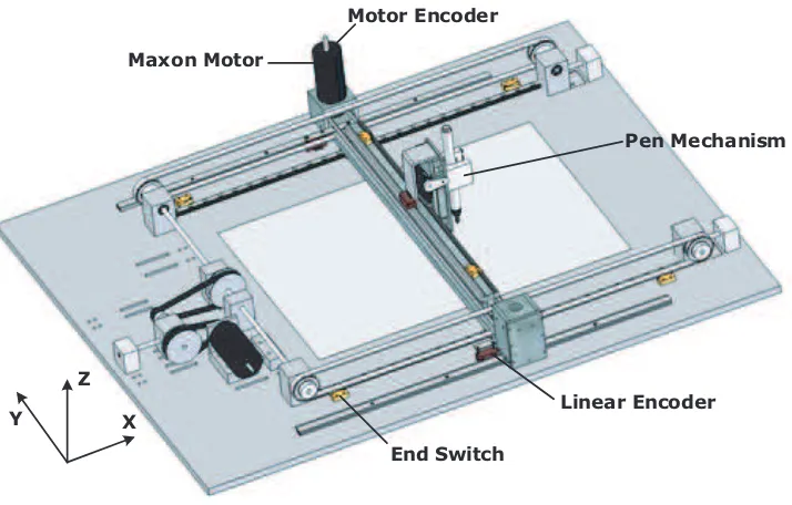
In this chapter the ViewCorrect Plotter setup is described extensively. First the specifications and requirements (2.1) are discussed. This is followed by a description of the mechanical (2.2), electrical (2.3), software (2.4) and safety parts (2.5). Figure 2.1shows the ViewCorrect Plotter.
End Switch
Linear Encoder Pen Mechanism Motor Encoder
Maxon Motor
Y X
Z
Figure 2.1: ViewCorrect Plotter.
Figure A.5(a) shows a schematic topview of the ViewCorrect Plotter with all the named com-ponents.
2.1
Specifications and requirements
This section describes the current specifications and requirements.
2.1.1 Specifications
• Direct Current (DC) Maxon motors are used for the x- and y-axis. Models of these motors are available in the model libraries of 20-Sim. The motors are controlled by Pulse Width Modulation (PWM).
• End switches are used to detect reaching end of rail. If an end switch is reached, then enough time is available to stop the mechanism safely.
• The position measurements is done by motor and linear encoders. The encoders provide feedback for the controllers.
• The drawing area is a A3-size (420 by 297 mm).
2.1.2 Requirements
• The setup should be easy accessible, because of demonstrating purposes. Changing paper should be a simple operation, because this occurs frequently.
• Safety is a important part of a test and demonstration setup. The setup has to be robust and has to designed in such a way that damage by faulty control or human faults are prevented.
• The setup has to be designed to be prepared for distributed control.
• The setup must be equipped with a demonstration button. When this button is activated, a demonstration will start. However this demonstration button is not implemented yet. • The maximum velocity should be limited to 0.5 m/s. This is due to safety reasons, but this
velocity is still fast enough to make a demonstration interesting to see. Due to the current status of the setup, the setup is still open which might be hazardous for bystanders, the maximum velocity is set to 0.2 m/s.
• The size of the plotter and his peripheral equipment should not exceed the size of a lab table.
2.2
Mechanical
Most parts of the plotter are made of aluminum. The axes are made from steel rod. The base plate is made from hardened aluminum. The weight of plotter setup is 18 kg. The rotation of the motor is converted to a translation by toothed belts and pulleys. The guidance system is implemented by rails.
The z-axis is the movement of the pen. It has two positions, on and off the paper. This movement is implement by a servo motor and an up and down mechanism. The x-axis is the longest side. One motor is connected to a steel wire axis which drives both sides. The setup is prepared for driving each side with a single motor. The y-axis is driven in the same way as the x-axis. The pen mechanism moves along a guidance rails back and forth. The mechanical part of the setup had still some shortcomings, which are described in the following subsections.
2.2.1 Improvement of mechanical parts
Some mechanical parts, especially the x-axis pillars with bearing, were not constructed precise enough. These pillars were pulled straight using screws, which harmed the construction more and more by time. Also the movement of the y-axis showed a non-linear behaviour caused by the construction. These shortcomings have been repaired partly in this project.
2.2.2 Redesign of the pen mechanism
The current design of the pen mechanism is new. In the previous project the pen was fastened with tie wraps. The redesign and realization of the pen mechanism is described in Appendix
A.1.
2.2.3 Linear encoders
moving perpendicular to the x-axis and during operation it will give information about possible friction or position error between the two sides of the x-axis. Especially when each side will be driven by a single motor in future projects. In the previous project, the linear encoders were not implemented. The design and realization of the implementation of the linear encoders is described in AppendixA.3.
2.3
Electrical
To control the setup a Embedded Control System (ECS) is used. The ECS consist of a PC/104 (Seco, 2007) with an Anything I/O board (Mesanet, 2007). The PC/104 with an Anything I/O board is already used in other setups at the CE laboratory. A PC/104 is a Personal Computer (PC), but with a different physical construction. It is based on a stackable circuit board. The Operating System (OS) system on the PC/104 is a Linux kernel with a real-time package. This makes it possible to run software from 20-Sim or gCSP.
The PC/104 is connected by a Peripheral Component Interconnect (PCI) bus with the Anything I/O board. This board has 72 general purpose Input/Output (I/O) ports connected to an Field Programmable Gate Array (FPGA). These I/O are available on three 50 pin connectors. The board is stacked on the PC/104.
At the start of this project electronic hardware from the Production Cell were used. A switchboard (van den Berg, 2006) was used to connect to different signals to the end switches, servo motor and encoders. A motor amplifier, H-Bridge (van den Berg, 2006), is used to drive the Maxon motors. However the switching board was not suitable to be used for the ViewCorrect Plotter setup. The linear encoder and the servo motor can not be connected to this board, it contains unnecessary expensive components and for distributed control the board can be simplified. Therefore a new electronic board and named as Motor Control Block (MCB) is designed in this project. The design and realization of the printed circuit board for the plotter I/O is described in AppendixA.4. Figure2.2 shows a schematic view of the electronics.
ECS
2.4
Software
Two types of software are written for this setup: real software for the PC/104 and the firmware for the FPGA hardware.
2.4.1 FPGA configuration file
The FPGA at the Anything I/O board has to be configured. The current FPGA configuration is the configuration of (Groothuis, 2004) extended with possibility to generate multiple PWM signals with different frequencies. In the old situation, it was only possible to generate a fixed PWM frequency for all PWM signals at 16.3 kHz. This is implemented in this project because of the redesign of the pen control.
Redesign of the pen control
Another aspect of redesign in this project is the pen control. The pen is driven by a servo motor. The servo motor and thus the position of the pen is controlled by a PWM signal. In the previous design the pulse was generated from the plotter software. In order to generate a pulse with a width resolution of 0.1 ms, a clock frequency of 10 kHz in needed in the plotter software. This is a high and undesired requirement for the plotter software. The redesign and realization of the pen control and thus the current FPGA configuration is discussed inA.2.
2.4.2 Plotter software
The plotter software is needed to use the setup. The previous plotter software was developed with 20-Sim. The movements of the plotter were limited to motion profiles which are not suitable for drawings. The current plotter software is designed in gCSP. This is described in Chapter
4. The CE- and ForSee toolchain is used to send the plotter software to the setup (Buit, 2005) (Posthumus, 2006).
2.5
Safety
In the setup, a couple of safety measures are implemented. In normal operation mechanical parts do not interfere with each other. Due to faulty control software or human faults, it is possible that a moving part is going to collide with other parts. These collisions are prevented by use of end switches. In case an end switch is hit, the moving part is stopped by actively braking the responsible motor.
An extra safety measure will be a emergency stop and a brake stop. An emergency stop is the highest level of safety and disconnects the voltage supply. A brake stop will brake electronically the motors. The difference between both stops is that pressing the emergency stop the moving parts are losing velocity by friction or collision. In case of a brake stop the moving parts are stopped electronically, but the setup is still connected to the power supply. Last two described safety measures are not implemented in the current setup.
2.6
Conclusion
• The pen mechanism has been redesigned and implemented. This mechanism can replace the pen easily and is prepared for future projects with another device like a milling cutter or inkjet head.
• The FPGA configuration file is extended with possibility to generate multiple PWM signals with different frequencies to be able to control the pen height.
• A MCB is designed and realized to process the plotter I/O. The MCB has the same form factor and is stackable with the existing CE H-bridge PCB (van den Berg, 2006) to a com-plete electronic circuit to control a DC motor with an I/O board. The board is equipped with an additional I/O connector for measuring or extension with additional electronics. The additional connector is interconnected with the connector to the I/O board. Conse-quently, it is possible to measure the signals at the I/O board during operation.
Due to lack of time some features of the ViewCorrect Plotter setup have not been implemented. At this moment, paper is fixed to the bottom plate. This should be replaced with some sort of clipper.
Besides a demonstration button, an emergency stop button and a brake stop button should be implemented. The demonstration button should be connected to a button connector of the MCB and a software process should detect a change of state and start a demonstration program stored in flash memory of the PC/104. The brake stop should also be connected to a button connector of the MCB. A predefined process in the FPGA configuration file should process this to a brake signal to the H-Bridge. The setup is still open, consequently dust and dirt can harm the construction. Besides it might be hazardous for bystanders, because the plotter can move with high velocity. It is recommended to make some sort of transparent cap.
If higher accuracy is needed it is recommended to redesign part of the gear of the x- and y-axis, because visual inspection shows still some non-linear behaviour. This was also visible in the validation of model that describes the behaviour of the ViewCorrect Plotter setup.
3.1
Introduction
Modelling and simulation is used for various parts of the project. The model of the ViewCorrect Plotter setup and its 3D animation extension model are used to design controllers, simulate the effects of changing dynamic parameters and for co-simulation with the plotter software. In case of co-simulation, the model will be used to test the plotter software together with its modelled physical environment.
The previous model of the ViewCorrect Plotter setup (Kuppeveld and Sprik, 2006) has been verified, but has not been validated. This model does also not include all properties of the setup, like the consequences of differences in elasticity in the belts between both x-axes.
This chapter describes the new model (3.2) and its validation (3.3), the design of the con-trollers (3.4) and a 3D model (3.5).
3.2
Model of the ViewCorrect Plotter setup
The current model is divided into five functional submodels. This division makes it easier to reuse the separate models for controller design or co-simulation. Figure 3.1shows the top level of the model.
DA-AD Converter ViewCorrect Plotter Controllers Safety
Data Input
Figure 3.1: Top level model of the ViewCorrect Plotter setup.
Data Input: The data input is a motion profile for the plotter. The motion profile can be a motor signal profile or a motion profile generated by the drawing to motion translator. This profile contains a motion to make a user-designed drawing. The drawing to motion translator is discussed in section 4.4. The data input submodel is connected to the controllers.
Controllers: This submodel contains the two controllers for the x- and y-axis. The design of the controllers is discussed in section 3.4. Another part is the control for the z-axis. This is a fixed value for the up or down position of the pen.
Safety: In this model, two safety measures are included. The first safety measure is a duty cycle limiter, which limits the steering value to a maximum (software safety measure). This safe value corresponds to a duty cycle, where the motor can prevent a collision with the pillars in case an end switch is hit. The second safety measure is the usage of end switches (hardware safety measure). In case an end switch is hit, the motor will brake and the duty cycle becomes zero. The controllers and the safety layer are embedded in the plotter software. This is discussed in section 4.5.
Digital to Analog (DA) and Analog to Digital (AD) conversion: The input for the actuators is converted to an analog signal. The signals from the sensors are converted to the digital domain.
Plant model ViewCorrect Plotter: This submodel contains the dynamic model of the plant. The structure of the plant model is depicted in Figure3.2. It is split up inH-Bridge,DC-Motor
a bond graph model with parameters from the datasheet. This model contains less details as the model from the 20-Sim motor library. However the missing details, like temperature of the motor, are not needed for co-simulation or controller design. The model of the y-axis has been adapted to include the consequences of the elastic differences in the belts between both x-axes.
DC-Motor
H-Bridge Mechanical
Figure 3.2: Structure plant model ViewCorrect Plotter.
The details and parameters of the model can be found in AppendixB.1. The validation of the model is described in the next section.
3.3
Validation of the ViewCorrect Plotter setup model
The model is validated, because it results into a more correct and accurate model. This is needed for the co-simulation case study, which is described in section5.5. An incorrect or not accurate enough model can give the idea that the software might be right while this is not the case. The model described in the previous section is validated in two parts.
The first part are the submodels data input andDA and AD conversion and the motor part of the plant model. The motor part of the plant model is the H-bridge and the DC-motor. The second part is the complete plant model, data input and DA and AD conversion. In this way the model is validated more accurately.
The motor model produces significant better results as the previous motor model of
(Kuppeveld and Sprik, 2006). Now the difference between model and the real setup is at the most 0.5 percent for both axes. The results can be found in Figure B.2.
The complete model, but still without the controllers and safety submodels, is validated after the first part validation using a steep motion profile. The estimated parameters of the friction, caused by bearings and guidance rails, have been changed as a result of the validation results. The results and figures with the simulation and measuring data can be found in Figure
B.3. The differences between the simulated and the measured data is below five percent. From this analysis it can be concluded that the model is accurate enough for controller design and (co-)simulation. The next section describes the design of the controllers.
3.4
Controllers design
The motors needs to be controlled in such a manner that the position of the pen follows the lines of a given drawing. The control variable is the angular position of the motor, which represents a certain movement of the pen. The maximum velocity specifications of the motion profile and accuracy of the plotter can be found in section 2.1.
move independently, so two controllers will be designed. The parameters are determined with the Ziegler-Nichols method (Astrom and Wittenmark, 1997).
As shown in the results in Figure B.4, the designed PID controllers can fulfill the specifica-tions.
The complete model as depicted in Figure 3.1 is validated, the results are shown in Figure
B.5. The error between simulated and measured encoder pulses is periodical during a motion. It looks like the dynamics are caused by the gear construction, because the number of periods is a multiple of the number of rotations of the motor axes.
3.5
3D animation extension of the model
A 3D animation is made using the 20-Sim animation toolbox. The 3D model is coupled to the dynamic model, but this is not necessary. The animation might be used stand alone, like a real-time visualization moving along with the plotter. The 3D model visualizes the movements of the ViewCorrect Plotter setup. Animating the 3D model with the simulation data from the dynamic model enables a quick insight in the correct functioning of the setup. It can be used for a couple of reasons. First it can be used to verify the working of the model as a whole. Secondly it can be used for demonstrating purposes. Besides it will be used in the visualization of the co-simulation between 20-Sim and gCSP. This is discussed in Chapter 5. Figure 3.3shows the 3D animation model.
Figure 3.3: 3D animation model of the ViewCorrect Plotter.
3.6
Conclusion
The existing model of the ViewCorrect Plotter setup is adjusted and validated. The difference between simulated and measured parameters is less than a maximum of five percent. The 3D animation model is made for enabling a quick insight to verify the dynamic model as a whole and for demonstrating purposes. Controllers for both axes have been designed according the Ziegler-Nichols method. The accuracy of the model is 0.03 mm during a motion with a maximum velocity of 0.2 m/s and 0.005 mm (1 pulse) when the motion is finished for the x-axis. For the y-axis, these parameters are 0.1 and 0,04 mm (1 pulse).
recommended to have a port-based and configurable with details motor library and a reusable model of a DC motor controlled by a PWM signal.
The complete model of the ViewCorrect Plotter setup is validated with a maximum velocity of 0.2 m/s due to safety reasons. If the setup is safe enough as specified in section 2.1, the model should be revalidated with the specified maximum velocity of 0.5 m/s to obtain the new accuracy.
4.1
Introduction
The construction of ViewCorrect Plotter is ready to draw everything. However with the previous plotter software, generated by 20-Sim, the movements of the plotter were limited to motion profiles which are not suitable for drawings. It is needed to have a workflow which allows the user to make a drawing in a Computer Aided Design (CAD) drawing package and plot this drawing with the plotter.
4.1.1 Workflow output of the plotter
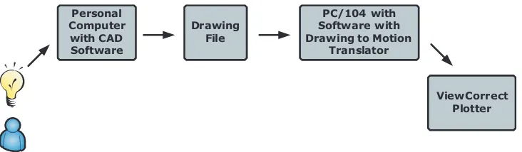
The workflow is depicted in Figure 4.1.
Personal
The PC on the left side is the starting point. The user has developed an idea for a drawing which has to be drawn by the plotter. The user designs his idea in a CAD drawing package. This idea will be stored in a file in a format which depends of the software tool used. This file contains all the information about the drawing. This file will be send to the PC/104. The PC/104 contains the plotter software. A part of this software is the control software. The control software controls the motors and other electronics. The input for the control software is the drawing to motion translator. This translates the file into the correct movements of the pen.
This chapter starts with the requirements and restrictions for the plotter software (4.2). This is followed with a analysis for a suitable drawing file (4.3) and a description of the structure of the drawing to motion translator (4.4). This chapter ends with the design of the plotter software in gCSP (4.5).
4.2
Requirements and restrictions plotter software
This section discusses the requirements and restrictions for the plotter software.
4.2.1 Requirements
The requirements for the plotter software are:
• Possibility to make the drawing in a CAD drawing package.
• Possibility to draw ’everything’ the user wants. The word everything is between quotes, because it is needed to keep the restrictions of a plotter in mind. These restrictions are discussed in the next subsection.
• The software should be designed according the top-down approach and tested with co-simulation.
• The drawing to motion translator discussed in section 4.4and the controller discussed in section3.4 should be embedded in the plotter software.
• The drawing to motion translator should limit the movements of the pen to the drawing area of the plotter, which is smaller than the end switch to end switch area.
• The software should contain a safety layer, which limits the steering signals to a safe domain. In case an end switch is hit, the safety layer should set the relevant steering signal to zero.
4.2.2 Restrictions
The ViewCorrect Plotter plots its output by moving a pen across the surface of a piece of paper. Consequently, the plotter is restricted to line art in contrast with raster graphics as with other printers. Solid filled objects can be drawn, but this requires exact knowledge of the pen point width. In case of a small pen point, this takes a lot of time. Consequently shaded filled objects are preferred. The plotter can draw complex line art, but at a low speed because of the inertia of mechanical construction of the x-, y- and z-axis. Drawing line art runs efficient with vector format drawings.
Vector format drawings are images that are described using mathematical definitions. This is in contrast to bitmap or raster format drawings. Raster images are described using pixel data. Every pixel contains the data for the corresponding colour. Most of the pen plotters use a vector based translator. Raster plotters can use a vector or a raster based translator. Consequently raster formats drawings are not useful for pen plotters.
4.3
Drawing file
4.3.1 File formats
As stated in the previous subsection, vector format files are suitable for plotters. Two kinds of vector format drawing files can be used. The first option is a file which contains all the information of the drawing. The second option is a file which represents the original drawing and contains all the information of the movements of the pen. Due to the existence of dozens of CAD drawing packages, a lot of different vector file formats exists. AppendixCshows a list with all common vector formats.
The first option means a file format in which the CAD drawing package stores the information of the drawing. The disadvantage of these formats is that they only contain information about the drawing, but not the content which describes how to make the drawing. Consequently choosing this option requires more work for the drawing to motion translator.
The second option means a plot command file format, which is generated from the original vector drawing format. Creating a plot file is a case of capturing the information that is normally sent to a plotter and saving it as a file instead. The file is produced by using standard plot/print tools within an OS. The advantage of plot files is that they represent the original drawing, including the order and movements of the pen. The most CAD drawing packages contain plot file generators. AppendixD.1gives additional information about a plot file.
more than ten times smaller than the normal CAD file formats. Plot files are written in a plot language. The next section describes the different plot languages.
4.3.2 Plot file languages
In the last decades multiple plot languages have been created. These languages contain com-mands with detailed information, for example draw a line from here to there. The de facto standard today is Hewlett Packard Graphic Language (HP-GL) or its successor HP-GL/2 (Oce, 2007). Other plotter manufactures created their own forms with extensions for their machines, for example Houston Instruments with Digital Microprocessor Plotter Language (DMPL). An-other common language is Gerber used by Printed Circuit Board (PCB) manufactures. HP-Printed Command Language (HP-PCL) and HP-Raster Transfer Language (HP-RTL) are more advanced printer and/or plotter languages. In AppendixDthe plotter languages are described in more detail.
Plot files in certain file formats can be viewed by special tools. The most common viewers read HP-GL(/2) files. Plot files in certain file formats can be converted to other file formats or edited. In this way plot files can be used to communicate about designs.
HP-RTL is a vector and raster plotting language and for the pen plotter only a vector plotting language is needed. HP-PCL is a more complicated language because of the supported features for laser printing. It uses HP-GL for the vector plotting. This leaves HP-GL, HP-GL2 and DMPL as options. All three languages describe the vector movements of the pen. HP-GL2 supports some extra features. DMPL is a form a HP-GL, but is less supported by CAD drawing packages, plot file viewers and the industry. This leaves HP-GL and HP-GL2 as options.
4.3.3 Conclusion
4.4
Drawing to motion translator
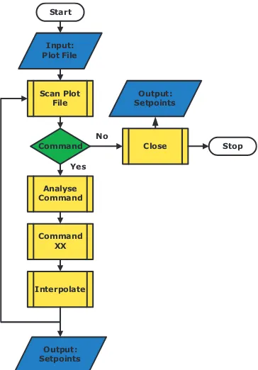
The drawing to motion translator is a combination of a couple of functions, decisions and input, which generate an output. The input is a file. The outputs are setpoints. In Figure 4.2 the flowchart of the drawing to motion translator is depicted.
Scan Plot
Figure 4.2: Flowchart drawing to motion translator.
Input: The input is a plot file written in HP-GL(2), generated by a drawing tool like AutoCAD or CorelDraw.
Scan Plot File: The plot file is opened and scanned on the occurrence of a semicolon, because every HP-GL(2) command is closed with a semicolon. On the occurrence of a semicolon, a command is found and the function Analyse Command is called. If no or no more semicolons are found the functionClose is called.
Analyse Command: The founded text is cleaned, i.e. all non-HP-GL(2) characters like white space are removed. After the command is found, a specific command function is called.
Command XX: All the needed parameters from the HP-GL(2) command are given to the functionInterpolate.
Interpolate: Setpoints are calculated in meters for the x- and y-motors. If the status of the z-as changes, the setpoints of the x- and y-motors are paused for a fixed time. In this way, the servo motor is able to move the pen up or down. The function Interpolate limits the setpoints to the maximal size of the drawing area for safety reasons. The setpoints for drawing a line are calculated according a cycloidal algorithm.
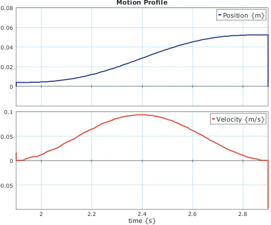
Figure 4.3 shows the pattern of the motion profile of function Interpolate. The duration of such a motion profile depends on the length of the line and a predefined parameter of the maximum velocity. The advantage of cycloidal profile for the velocity is that at the end of the command the velocity is zero. Consequently, drawing right or acute angles have no risk of overshoot. However this is not always the optimal way of drawing looking at the time aspect. For example, when the next line is almost in the same direction the plotter still stops between both lines, instead of just moving on without slowing down the velocity. However finding the optimal way of moving is a project in itself.
Motion Profile
Figure 4.3: Motion profile of a line.
4.5
Plotter software in gCSP
The plotter software is written in gCSP. The plotter software runs at the PC/104. The software is written in gCSP, because of the ability to design real-time CT-based software in a graphical application.
This section describes the design of the plotter software in gCSP. First it gives an introduction to gCSP. This is followed by a functional top level design and ends with a top level structure in gCSP.
4.5.1 Introduction in gCSP
(Hilderink et al., 2000). The CT library is based on the concept of the Occam language, which is a parallel programming language and CSP principles.
Besides code for formal verification of the CSP model can be generated from the model. The formal verification of the model can be done in FDR2 (FDR2, 2007). FDR2 is a model checker which is capable of analysing the models against properties as for example deadlock and livelock.
4.5.2 Functional top level design
From the requirements in the previous section a functional top level design is made. This is depicted in Figure4.4.
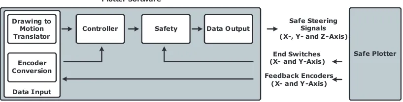
Figure 4.4: Functional top level design plotter software.
DataInput reads the encoder values and converts the pulses to meters, and the drawing to motion translator calculates the setpoints for the motors. Controller compares the reference values with the converted feedback , calculates a steering signal and generates control signals for the z-axis. InSafety the steering values will be limited to a safe domain and theSafety component detects if an end switch is hit. TheDataOutput component writes the data to the Anything I/O board, which sends the signals to the motors.
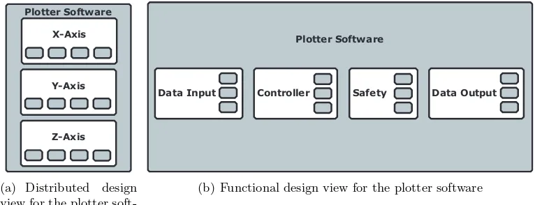
In order to be prepared for distributed control, a functional design does not seem to be a natural way of designing distributed software. It would be more logical to split the software into distributed components (X-, Y- and Z-axis) and divide these components into the functional components described in the previous paragraph. However a functional design gives a direct clear view of the structure of the software. In Figure 4.5 both views are depicted. The small grey blocks in the larger white blocks are in the left figure the functional components and in the right figure the distributed components. The dependencies between the components do not change in the different views.
Z-Axis Y-Axis X-Axis Plotter Software
(a) Distributed design view for the plotter soft-ware
Data Input Controller Safety Plotter Software
Data Output
(b) Functional design view for the plotter software
Figure 4.5: Two types of design views for the plotter software.
4.5.3 gCSP top level structure
In Figure4.6the top level structure of the plotter software in gCSP is depicted.
Figure 4.6: gCSP top level architecture of the plotter software.
The four components are implemented as processes. All processes work parallel in relation to each other. The details of the four processes are shown in AppendixF.
4.6
Conclusion
A workflow is analysed and presented allows the user to make a drawing in a CAD drawing package and plot this drawing with the plotter. The plot command file format is chosen as vector file format which is send to the ViewCorrect Plotter setup. This format represents the original drawing which is designed in a CAD tool, including the drawing order and the movements of the pen. HP-GL(2) is chosen as plot language. A drawing to motion translator is designed which can read a plot command file, written in HP-GL(2), and translates the different commands to setpoints for the motors. The setpoints are limited to the drawing area of the plotter for safety reasons. The drawing to motion translator calculates the setpoints according a cycloidal pattern. At the end of a draw command the velocity is zero and in the middle maximum.
The plotter software is designed in gCSP with a top down approach and with a functional design view. It is divided in four processes: DataInput reads the encoders and the drawing to motion translator calculates new setpoints, Controller computes new steering values from the feedback and reference values,Safety limits the steering values to a safe domain andDataOutput
writes these values to the Anything I/O board.
The plotter software is designed with a functional view. To be prepared for distributed control, it would be more natural to have a distributed design view. However, a distributed design view gives the software a less clear structure. In the current version of gCSP it is not possible to change between these views. It is recommended to have this possibility in gCSP.
No timing has been added to the plotter software. Previous projects concluded that the timed execution of (control) processes in the CT-library contains too much jitter. It is recommended to redesign timing dedicated for the Linux OS with real-time package instead of the current work around.
A cycloidal profile for the velocity is not always the optimal way of drawing looking at the time aspect. Future research is needed to find the optimal way of moving for the plotter.
5.1
Introduction
The plotter software written in gCSP and the model that describes the behaviour of the View-Correct Plotter setup, designed in 20-Sim, are connected to each other. In this way, it is possible to test the software with its physical environment without using the real plant. In order to test the generated code from gCSP together with 20-Sim, a co-simulation facility has to be designed. A lot of commercial co-simulation facilities are available, but they are dedicated to a specific design environment and only for connecting with another specific design environment. Currently no flexible framework exists for co-simulation. This project starts to address the requirements and analyse such a framework.
This chapter starts with discussing heterogeneous design approaches (5.2), details, require-ments and challenges of co-simulation (5.3). This is followed with a co-simulation facility frame-work (5.4) and a case study of testing the plotter software together with the model that describes the behaviour of the ViewCorrect Plotter setup(5.5).
5.2
Heterogeneous design approaches
A mechatronic system, like the ViewCorrect Plotter, is an example of a heterogeneous system. It consists of components belonging to different domains. These components are being described using different specification languages. Like VHDL for hardware or C for software. Two ap-proaches have been developed to design heterogeneous systems: the compositional approach and the co-simulation approach.
The compositional approach, Figure 5.1(a), tries to integrate the different parts into a uni-fied representation. This representation is used to design and verify global behaviour. The unified representation makes its possible to do full coherence and consistency checking. New specification languages can be added to the composition format. A major disadvantage of this approach is that it does not give the design engineer the freedom to choose the most suitable design environment. Examples of this approach are Polis (Polis, 2007) and Ptolemy (Ptolemy, 2007).
Figure 5.1: Two types of approaches for heterogeneous design.
allow for cooperation. Examples of this approach are VCI (VCI, 2007) and CoWare (CoWare, 2007). However both examples only deal with hardware/software co-design. Other examples like Data-Distribution Service (DDS) (DDS, 2007) and RT-LAB Orchestra (C´ecile et al., 2006) only deal with distribution of the data, not with issues like continuous time or discrete event models. A lot of commercial packages are available to connect only two design environments, like PSpice-Matlab/Simulink (EMA, 2007). A difficulty of the co-simulation approach is the checking for overall coherence and consistency due to the fact that the system is split up in multiple subsystems. In the next section, co-simulation is discussed more extensively.
5.3
Co-simulation
Co-simulation is simulation of a heterogeneous system of which parts are interacting and dis-tributed over more than one simulation engine connected with a co-simulation bus. In fact it is a joined simulation of the different parts of the system by using simulation engines and abstraction levels appropriate to each part. It can be used between different design environments, describing different domains or components and between different PCs.
A major reason to use co-simulation is that it allows for combining separate design groups, like software and control engineering. This results in a heterogeneous system design and verifi-cation environment, instead of only the design and verifiverifi-cation of the separate part or domain. This design and verification can be done at different abstraction levels, so it is a verification technique in the entire design cycle. Other additional advantages are (re-) using of models developed in other design tools. Increase of simulation speed when simulation takes places at multiple processors. Besides it allows for cooperation of design engineers at different places. Two types of co-simulation are developed: untimed and timed simulation.
5.3.1 Untimed and timed simulation
Untimed simulation considers the functional behaviour of the overall system. Untimed co-simulation is event based. The data exchange between the design environments is controlled by events. Untimed co-simulation only verifies sequences of operations. Timed co-simulation considers both functionality and (real-) timed behaviour, now timing aspects are included in the functional behaviour. The major problem for timed co-simulation is synchronization between the different design environments.
Untimed or timed co-simulation can be used at different stages of a design cycle. At the beginning untimed co-simulation can be used to verify the functional behaviour of the high level definition of the various components or functions of the system. Later in a design cycle, (real-) timed co-simulation can be used to verify the behaviour of the refined description of the components.
5.3.2 Requirements
The co-simulation facility is described with the following requirements. A major requirement is the first:
• The results of co-simulation should be same as when the different parts where modelled in the same design environment. Consequently the co-simulation facility should not have any effect on the results of the simulation.
• The design environment interface should be generated automatically. This allows the user, regardless of communication protocol or architecture, to concentrate on simulation. Besides it will be easy to use for engineers of other disciplines, because it requires no knowledge of other design environments.
• The data communication should be synchronized, especially during timed co-simulation. All design environments should be at the same point of execution of the overall system model.
• A Graphical User Interface (GUI) or 3D animation model is needed to visualize the impact of design decisions to other design disciplines and to observe problems.
• Able to perform the co-simulation distributed at different workstations/places.
• A common parameter database is needed to strengthen the value of the co-simulation pro-cess. In this database all (common) variables/constants are stored for checking purposes.
The requirements mentioned in the previous section lead to a couple of challenges.
5.3.3 Challenges
Model computation
Computation of the parts might become a problem, when they are simulated with different step sizes or consist of parts simulated in the continuous time or discrete event domain. If all parts use the same step size for their computation, no problems exists related to data availability. However this is not always possible. If some part calculates its state at a lower step size as the other interacting parts, the other parts need data interpolation in this step to avoid erroneous simulation. Figure5.2shows an example of two parts, where one simulation process operates at a higher step size and needs data interpolation.
t1
t1b t
2Figure 5.2: Two simulation processes with different step size.
Data interpolation
Continuous time and discrete event
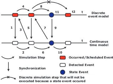
A design environment can work with a discrete event model or a continuous time model. In continuous time models, time is a global variable and advances by (variable) integration steps. In discrete event models, time is a global notion for the overall system. It advances discretely at the occurrence of an event. Continuous time models are computed as discrete time models. Synchronization of these different time models might be problem. Besides, the discrete event simulator must detect state events. “A state event is an unpredictable event, generated by the continuous time simulator, whose time stamp depends on the values of the state variables (for example: a zero-crossing event or a threshold overtaking event)” (Gheorghe et al., 2007). At detecting a state event, the discrete simulator has to advance until the time of the state event, instead of advancing with a normal simulation step. In Nicolescu et al. (2007) the operational semantics for synchronization in continuous/discrete models are presented. The basic idea is illustrated in Figure 5.3. It uses the Discrete EVent System Specification (DEVS) formalism (Zeigler and Kim, 2000). This is an abstract simulation mechanism and enables event-based, distributed simulation. The implementation for a co-simulation interface of this formalism is presented in (Gheorghe et al., 2007).
Discrete event model
Continuous time model 1
Discrete simulation step that will not be executed because a state event occured Synchronization
Figure 5.3: Continuous and discrete-event models synchronization (Nicolescu et al., 2007).
The discrete event simulator starts with executing all processes and updates all signals sensitive to the notified events at zero time. The continuous time simulator gets a time stamp of the next output event of the discrete event simulator (1). The continuous time simulator advances to the time stamp (2) and switches to the discrete event simulator (3), which advances to the event time stamp (4) and this cycle restarts again.
discrete event simulator (7). The discrete event model advances to the time stamp and executes all processes that are sensitive to this external event (8). An advantage of this model is that it does not need a rollback if a state event is detected.
Model ordering
The order of computation of the different parts might become a relevant issue. A part might have import and export variables. If the export variables only depend of their own states and time, the order of computation is not important. This is depicted in Figure5.4(a). The different parts can be calculated in parallel in random order. However if a direct relation between import and export variables exists, it is needed to have specific order of computation. This is depicted in Figure 5.4(b). Now the different parts can only calculated in a certain order.
No direct dependencies
Figure 5.4: Dependencies between simulation processes.
The relations between the different parts might result in an algebraic loop. This can only be solved by iterative methods. If the algebraic loop can not be eliminated, the only solution is to use an algebraic loop solver. This forces the simulation engine to do a lot more computations.
It is needed to know the different dependencies between the processes, a dependency graph. This dependency graph is used to investigate the overall system with respect to the order of computation. An automatic solution for a dependency graph, only looking at the import and export variables, is not possible. The rate of change of a export variable investigated with respect to the rate of change of the import variables might give the idea of a direct relation. However the cause may be a non-linearity of the component. A integrated solution for a dependency graph would be a translation of the part into a formal specification language. The combination of these code blocks, from the different design environments, represent the dependency graph. A similar approach is used in gCSP models and FDR (see subsection 4.5.1).
5.4
Co-simulation facility framework
From the requirements, a framework is chosen to handle the described challenges. The co-simulation facility uses a client/server approach. The co-co-simulation server is a separate unit which controls the overall simulation process. The design environments are clients and exchange data via the co-simulation interface and the co-simulation bus with the co-simulation server.
in-terfaces requires more manual activities, to know for example the interacting with other design environments, because the overall system information is missing. With an extra program in the co-simulation server the design environments and the interfaces need no extra intelligence and therefore the interfaces can be generated easier automatically. A disadvantages of putting all the intelligence in the server is that this creates a higher data transfer rate, because now all the data, for example due to data reconstruction, needs to be send to the clients.
Due to the fact that the co-simulation facility should be able to be distributed over different workplaces, the co-simulation bus will be implemented over a Local Area Network (LAN) or even a Wide Area Network (WAN) and uses Ethernet as data link layer and Internet Protocol (IP) as network layer protocol. Two common transport protocols can be used; Transmission Control Protocol (TCP) and User Datagram Protocol (UDP). In AppendixJboth protocols are discussed extensively.
The main advantage of TCP is its own correction protocol; data will be send and faults are corrected. The disadvantage is that no knowledge exists about how much time it takes to repair faulty transmission. Consequently, it is not known how long it takes to send a packet of data. Another disadvantage of TCP is that broadcasting messages is not possible. UDP has no correction protocol, data will be send, but it is not checked if the data is arrived. An advantage is that faster transmission speeds and broadcasting messages are possible.
The best option here is to use TCP for the untimed and timed simulation, because of the reliability and the simulation time requires no real-time demands. In case of a real-time sim-ulation TCP can be used, but that depends on the time constraints. Otherwise UDP has to used, because an own implementation of flow control is possible, which allows for higher real-time constraints. However along with UDP, it is needed to have error correction to handle for example missing or duplicate data packets.
The co-simulation facility framework is depicted in Figure 5.5. The components of the co-simulation facility framework are described in section5.4.1.
5.4.1 Description of components of the co-simulation facility framework
Bus Interface: The bus interface is part of the interface, but only takes care of exchanging data with the bus. The implementation depends on the technical implementation of the bus.
Bus Library: The bus library contains all the functions or processes to connect and exchange data between the interface and the co-simulation bus. The functions support the communication protocol and are specified to technical aspects of the bus.
Configuration File: This file is developed form high level system analysis and contains the architecture of the heterogeneous system. From the architecture the dependencies of the dif-ferent subsystems are derived. This information is transferred to the sequence controller. The configuration also contains all common information about the simulation of the sub models, like simulation step size, continuous or discrete time. This is needed to initialise the timing component. All these information can be displayed at the GUI.
Co-Simulation Bus: The co-simulation bus transfers all data to and from the interfaces and server.
Co-Simulation Server: The server is in charge of the overall process. The server decides the order and synchronization of computation and interpolates data if necessary. Besides it checks if common variables of the subsystems are similar.
Data Storage: In order to interpolate data, the values of earlier moments have to be stored. These values will be stored at the server.
Data Transfer: Data Transfer transfers all data to the design environments and from the data storage according the communication protocol.
Design Environments: The design environment is software application suitable to do the design and verification of the subsystem.
Graphical User Interface (GUI): The GUI is the visualization of the overall system. The GUI gets the data to visualise the overall system from the data storage. If a design environment is capable of providing a visualisation of the overall system, it might not be needed to have a animation of the system on the GUI. Information from the configuration file and from the parameter relationship component can be displayed at the GUI.
Interface: The interface provides a connection between the design environment and the co-simulation bus.
Interface Library: The interface library contains all the functions or processes to connect and exchange data between the design environment and the bus-interface. The interface library is not aware of technical aspects of the bus. The implementation of the interface will depend on the structure of the design environment.
Parameters Relation File: This file contains all the variables/constants of the system and is part of the configuration file. In case the subsystems share variables, before the start of the sim-ulation it will be checked if they are similar. Mismatches or other information can be displayed at the GUI.
Scheduler: From the dependency graph, the order of how the system has to be calculated becomes clear. In this order the different design environments will be executed. The scheduler commands the data transfer.
5.5
Case study: Co-simulation with 20-Sim and gCSP
This case study will give more insight in the value of the co-simulation facility framework. It should be clear that this is a long term project and that this case study is a start of the complete co-simulation facility. The main purpose is to test the plotter software, but it also will look at the co-simulation facility in a heterogeneous design view.
The idea is that the plotter software, discussed in Chapter4, and the I/O and plant part of the model, discussed in Chapter 3, do not need to be changed for co-simulation. However with the current version of 20-Sim it is needed to use a Dynamic Link Library (DLL) to export or import data. The DLL has to contain predefined functions which are supported by 20-Sim. The plotter software reads and writes data from and to the hardware with link drivers. Therefore in gCSP it should be possible to replace the implementation of the link drivers with TCP/IP drivers instead of the Anything I/O board link drivers. In (ten Berge, 2005) such kind of link drivers have been designed. However tests concluded that these network and remote link drivers do not work under Windows. Therefore it is decided to start from scratch and write new cross platform link drivers for UDP or TCP communication over IP.
The bus interface is implemented with a Socket and a Linkdriver class. The network and remote link drivers’ structure is not yet implemented in these classes. In Socket the basic functions for communication are implemented. The Linkdriver acts as a server or a client and uses functions from Socket. The co-simulation server is not implemented in this case study. Because of the fact that timing is not included in the plotter software, it is synchronized with timing from 20-Sim. Therefore 20-Sim acts as a server and gCSP as client. The co-simulation bus uses TCP as transport protocol. Timing is not included in the plotter software. If this is included, timing can be simulated with SimTimers (ten Berge, 2005). However it should be investigated if the simulated timing behaviour is conform the real timing in the CT-library.
In Figure5.6the framework of the case study is depicted. The plotter software sends steering signals applied as PWM values to 20-Sim. These values are converted to the analogue domain and sent to the plant model. In the plant model the motors, controlled with the PWM signals, are moving the plotter construction. The values of the encoders and end switches are given to the plotter software. The co-simulation server is not implemented in this case study and therefore circled with a dotted line. Now 20-Sim acts as a server.
Co-Simulation Bus
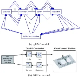
In the following figures, the gCSP and 20-Sim models are depicted with their co-simulation facility. The network and remote link drivers’ structure is not yet implemented. Therefore an extra process is needed in the plotter software. This process called CoSimulationInterface
replaces the link drivers as depicted in Figure4.6.
(a) gCSP model
DA-AD Converter ViewCorrect Plotter
Co-simulation
Facility 20-Sim
(b) 20-Sim model
Figure 5.7: Co-simulation facilities in both design environments.
5.5.1 Results
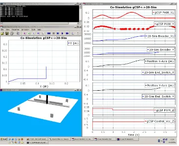
Two tests are performed for the plotter software. A functional test with simulated time under normal operation circumstances, which shows the correctness of the drawing and control part. The second test was a functional test with simulated time with deliberate disorder to show the correctness of the safety part. Figure5.8shows a screenshot of all the programs running. In the left upper corner the plotter software is shown. On the right side a 20-Sim simulation plot of the transfered and additional signals. On the left lower side the 3D animation model is depicted. Above the animation, an x-y simulation plot shows the movements of the plotter. Figure 5.9
Figure 5.8: Screenshot co-simulation with 20-Sim and gCSP.
Co-Simulation gCSP<->20-Sim
0 0.02 0.04 0.06
0.08 gCSP PWM_X1
0 0.5 1 1.5 2
time {s}
0 0.5 1 1.5
20 Sim End_Switch_X
Figure 5.9: Case study: Testing safety part plotter software.
Co-Simulation gCSP<->20-Sim
Figure 5.10: Case study: Critical code error in plotter software.
5.5.2 Conclusion of the case study
The strength of co-simulation for testing software has been proved by the fact that the functional correctness can be verified and errors can be fixed before running the software on the real setup. In this way the ’first time right’ principle of developing software becomes an easier goal, because now the software can also be verified on functional and timed behaviour. However the results depends on the quality of the model. An incorrect or not accurate enough model can give the idea that the software might be right while this is not the case. Co-simulation allows for concurrent engineering, because the software can be developed while the setup might be still under construction. Another advantage is that co-simulation does support rapid prototyping, because features can be verified in different design environments without the need to build the setup. It can be concluded that co-simulation is a powerful tool in heterogeneous system design and especially for testing embedded software in a model-driven design approach, which brings engineers from different disciplines in a natural way together.
This case study has shown the necessity for a configuration file, because both simulators have to operate at a same simulation frequency. Now this has to be edited manually which is susceptible for human faults. Automatic interface generation is not included in the current facility, although it is rather straightforward to implement. Looking at this case study, it is recommended to have automatic interface generation for different design environments, because each design environment has its own structure for cooperation with extern tools. Another fact that was illustrated during the case study is that different names belonging to the same variables or constants require good communication agreements. However a configuration file and a parameter relation file, as stated in the co-simulation facility framework, can overcome these challenges.
5.6
Conclusion
facility framework is designed. A case study is performed to evaluate co-simulation. In this case study, the plotter software, designed in gCSP, is tested together with the 20-Sim model of the ViewCorrect Plotter setup. In this way, the plotter software is verified on functional and timed behaviour without using the real setup. It can be concluded that co-simulation is a powerful tool for verification in a model-driven design approach for embedded control systems, which brings engineers from different disciplines in a natural way together. However the success of co-simulation depends on the quality of models used for testing, like the model used for testing the software, and whether the design environments allow for cooperation.
6.1
Introduction
A couple of times the ViewCorrect Plotter setup demonstrated unexpected behaviour. Because of the fact that the setup consist of several components like electrical, hardware and software, analysing the cause of this behaviour is not easy. Besides, the behaviour occurred at a time a new software application of the ForSee toolchain was used. This challenge requires a systematic workflow of verifying (individual) system performance characteristics. Such a workflow for the used components is not yet available at the CE laboratory. In the next section a systematic workflow is presented to isolate and solve a cause of unexpected behaviour. The workflow uses parts of the Failure Mode, Effects and Criticality Analysis (FMECA) approach as presented in Blanchard and Fabrycky (Blanchard and Fabrycky, 2004). This approach is translated to an workflow which is useful for failure analyses specialized at research setups at the CE laboratory. The words fault and failures are used as defined in (Jovanovic, 2006). A fault in a system is a defective value in the state of a component or in the design of a system. Failure is the behaviour of a system that deviates from that which is specified.
6.2
Systematic workflow
Finding a cause of a failure is finding how the failure is introduced in the system. Further it is needed to note the effect on other elements of the system and the system as an entity. This asks for identifying possible faults in the system, determine the causes of failures, determine the consequences of failures and identify failure detection means. In order to design and construct reliable systems, this failure analysis has to be done from the beginning of a project (”before the fact”). However, due to lack of time or bad system engineering this is not always implemented and happens ”after the fact”.
In general a research setup at the CE laboratory consists of components of different domains; mechanical and electrical engineering, and a ECS. The mechanical part is often a construction, where a subpart is able move in order to do a specific task. The electrical part is divided into two subparts. Firstly the actuators and sensors, secondly the PCBs to process the signals to the actuators and from the sensors to a I/O interface of the ECS. The ESC processes the available information from the sensors to steer the actuators. The ECS consist of hardware and software. The software is designed and created on a development PC with software applications, like 20-Sim and/or gCSP. The software is adjusted for and send to the hardware with other software applications, like the ForSee toolchain. In each of these domains failures might occur. Figure
(1) Identify
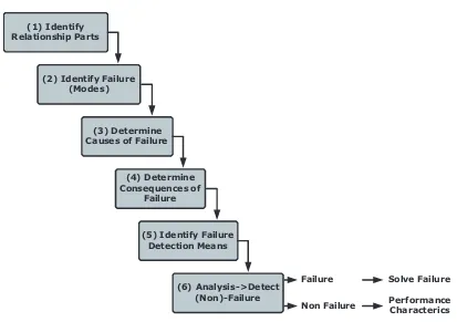
Figure 6.1: Systematic workflow for failure analysis.
1. Identify the relationship between the different parts and/or levels of the system. This helps with getting a global view and finding the effects of failure.
2. Identify, which failures are likely to happen. This can be extended with the failure mode, which is the manner a system element fails to accomplish his function. For example a sensor may fail cause of low power supply or dirt.
3. Determine the cause of the failure. This means analysing the environment, equipment, material or procedures. Examples of causes are a software coding error, defective materials or abnormal equipment stresses during operation.
4. Consider the consequences of the failures on the same, higher and overall system level. The results of step one can be helpful here.
5. Address ways to detect identified failures in the setup, with for example aids, tools or measurements devices.
6. Analyse the identified failures with the detection options described in step five. This step results in detection of a failure or detection of non-failure. In case of a failure, plans have to be made to solve the failure. In case of a non-failure, performance characteristics have to be reported. This starts with analysing the lowest level components of the system. After that the higher level components are analysed together with the lower level components or alone. The advantage of this approach is that in this way components from lower levels can be used for detecting failures at a higher level. This gives the advantage of using the existing components instead of making new components only for test purposes.
part. Failures