Bayesian Survival Analysis without Covariates
Using Optimization and Simulation Tools
Yasmin Khan1, Athar Ali Khan2
Research Scholar, Department of Statistics & Operations Research, Aligarh Muslim University, Aligarh, Uttar Pradesh, India1
Professor, Department of Statistics & Operations Research, Aligarh Muslim University, Aligarh, Uttar Pradesh, India2
ABSTRACT: Weibull and exponential distribution is one of the most important and flexible distributions in survival analyses. In this paper, Bayesian regression analysis without covariate with censoring mechanism is carried out for intrauterine device (IUD) data problem. Throughout the Bayesian approach is implemented using R and appropriate illustrations are made.
KEYWORDS: Bayesian Inference, Right censoring, LaplaceApproximation, Survival function.
I. INTRODUCTION
The analysis of survival data is a major focus of the statistics business. The main theme of this chapter is the analysis of survival data using two parametric models, namely Weibull and exponential. These models are very flexible and have been found to provide a good description of many types of time-to-event data. These are the distributions which occupy a central role because of their demonstrated usefulness in a wide range of situations. There are many potential life time models but these models are used quite effectively to analyze skewed data sets and give best data fit.
Weibull distribution has two parameter, shape and scale. Its density, survival and hazard functions, respectively are:
a ab
y
b
y
b
a
y
f
(
)
exp
1
ab
y
y
S
(
)
exp
Where a > 0 and b > 0 are the shape and scale parameters respectively. Corresponding probability density, survival and hazard function of exponential model are:
b
y
t
S
b
y
b
t
f
exp
)
(
exp
1
)
(
Likelihood function for right censored data is,
i i
i i
n
i i i n
i
y
S
y
f
y
L
11 1
)]
(
[
)]
(
[
)
,
Pr(
Where
i is an indicator variable which takes value 1 if observation is censored and 0 otherwise. Section III begins with a brief discussion of the Bayesian analysis of intercept model based on the Weibull and then exponential distribution. There has been growth in the development and application of the Bayesian inference. The Bayesian inference enables us to fit very complex model that cannot be fit by alternative frequentist methods. To fit the Bayesian models, one needs a statistical computing environment. An environment that meets these requirements is the R (R Development Core Team [1]) software. In this paper, an attempt has been made to illustrate the Bayesian modelling by using the R language. The package used in the paper to get the posterior summary is LaplacesDemon Statisticat [2] which reveals the conceptual simplicity of the Bayesian approach for survival data analysis. This package has several optimization and simulation algorithms. The default optimization algorithm is LBFGS (Broyden-Fletcher-Goldfarb-Shanno). Also a very popular algorithm, i.e. the Nelder-Mead [3], is a derivative-free, direct search method which is efficient in small-dimensional problems. The LaplacesDemon offers numerous MCMC algorithms for simulation in Bayesian inference, and are, Random-Walk Metropolis (RWM), Metropolis-within-Gibbs (MWG), Delayed Rejection Metropolis (DRM), etc. This package provides a complete Bayesian environment to the user. Section VII provides a model compatibility study based on DIC and deviance criterion so that the choice of these two models can be justified for the data under consideration. Finally, in the last section a brief discussion and conclusion is given.II. RELATED WORK
A significant amount of work has been done for estimating the linear regression model for censored data khan and khan[4], Khan and khan[5], Khan et al[6], Collet[7] and Puja et al. [8] discuss the Bayesian survival analysis of head and neck cancer data and conclude that which therapy has give better performance for patients. In this paper all analyses and computation were undertaken using LaplacesDemon package available in R software.
III. BAYESIAN FITTING OF INTERCEPT MODEL WITH CENSORING
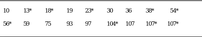
Here we want to make inferences about the response and intercept. In this section, we will consider these two models, Weibull and exponential models for the data which is discuss here are the time to discontinuation of the use of an IUD. The data in Table 1 refer to the number of weeks from the commencement of use of a particular type of intrauterine device (IUD), known as Multi load 250, until discontinuation because of menstrual bleeding problems. Data are given for 18 women, all of whom were aged between 18 and 35 years and who had experienced two previous pregnancies. Discontinuation times that are censored are labelled with an asterisk.
Table I: Time in weeks to discontinuation of the use of an IUD.
10 13* 18* 19 23* 30 36 38* 54*
56* 59 75 93 97 104* 107 107* 107*
The intercept model is in the form of
y
e
Where, a and b are shape and scale parameter and
X
,log(
b
)
X
~
N
(
0
,
1000
)
~
halfcauchy
(
25
)
IV. FITTING OF WEIBULL MODEL
Weibull distribution has two parameters, shape and scale. It can be denoted as
y
~
W
(
a
,
b
)
thus, the likelihood is
n i a i a ib
y
b
y
b
a
b
a
y
p
1 1exp
)
,
|
(
which implies log-likelihood as
n i a i a ib
y
b
y
b
a
b
a
y
p
1 1exp
log
)
,
|
(
log
Bayesian fitting of Weibull model for this data can be done in R by using function LaplaceApproximation and then
with LaplacesDemon. Its fitting includes codes for creation of data and definition of model. R codes to fit Weibull model is being described below.
A .CREATION OF DATA
LaplaceApproximation function requires data that is specified in a list. Though most R functions use data in the form of a data frame, Laplace's Demon uses one or more numeric matrices in a list. It is much faster to process a numeric matrix than a data frame in iterative estimation. For the above data of 18 patients with discontinuation time has given the survival times in weeks as a response variable. Since intercept is the only term in the model, a vector of 1s is inserted into design matrix X. Thus, X=1 indicates only column of 1s in the design matrix.
library(LaplacesDemon) y<-c(10,13,18,19,23,30,36,38,54,56,59,75,93,97,104,107,107,107) censor<-c(1,0,0,1,0,1,1,0,0,0,1,1,1,1,0,1,0,0) N<-18 J<-1 X<-matrix(1,nrow=length(y)) mon.names<-c("LP","shape") parm.names<-as.parm.names(list(beta=rep(0,J),log.shape=0)) MyData<-list(J=J,X=X,mon.names=mon.names,parm.names=parm.names,y=y)
There are J=1 independent variables (response variable). The R codes defined above must have a name specified for each parameter in the vector parm.names, and parameter names must be included with the data in a list called
as.parm.names. The user must specify the number of observations in the data as either a scalar n or N. If these are not found by the LaplaceApproximation or LaplacesDemon functions, then it will attempt to determine sample size as the number of rows in y or Y.
B. INITIAL VALUES
Laplace's Demon requires a vector of initial values for the parameters. Each initial value is a starting point for the estimation of a parameter. When all initial values are set to zero, Laplace's Demon will optimize initial values using a hit-and-run algorithm with adaptive length in the LaplaceApproximation function.
C. MODEL SPECIFICATION
Model<-function(parm,Data) {
beta<-parm[1:Data$J] shape<-exp(parm[Data$J+1])
beta.prior<-sum(dnorm(beta,0,1000,log=T)) shape.prior<-dhalfcauchy(shape,25,log=T) mu<-tcrossprod(beta,Data$X)
scale<-exp(mu)
w1<-log(scale)+log(shape)+(shape-1)*log(y)-scale*y^shape s1<--scale*y^shape
LL<-censor*w1+(1-censor)*s1 LL<-sum(LL)
LP<-LL+beta.prior+shape.prior
Modelout<-list(LP=LP,Dev=-2*LL,Monitor=c(LP,shape),yhat=mu,parm=parm) return(Modelout)
}
D. FITTING OF MODEL WITH LAPLACE APPROXIMATION
M1<-LaplaceApproximation(Model,Initial.Values,Data=MyData,Sample=1000,Iterations=10000)
The output summary is tabulated in Table 2 and Table 3.
Table 2:Approximated posterior summary of IUD data using LaplaceApproximation function with posterior mode, posterior sd and their quantiles.
Mode SD LB UB
beta -7.69 2.06 -11.81 -3.57
Log.shape 0.52 0.27 -0.03 1.07
Table 3:Simuated posterior summary of IUD data using sampling importance resampling in LaplaceApproximation function with posterior mean, posterior sd and their quantiles.
Mean SD LB Median UB
beta -7.55 1.64 -10.72 -7.42 -4.64
Log.shape 0.47 0.23 0.04 0.47 0.87
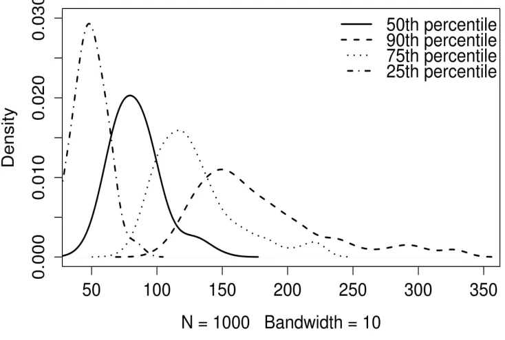
V. MEDIAN SURVIVAL TIME
Median survival time is the time beyond which 50% of the individuals in the population under study are expected to survive, and is given by that value t(50) which is such that S(t(50)) = 0.5. As we know Survival time distribution is always positively skew, the median is the preferred summary measure of the location of the distribution. Once the survivor function has been estimated, then it is easy to obtain an estimate of the median survival time.
The estimated median survival time, {t(50)}, is defined to be the smallest observed survival time for which the value of the estimated survivor function is less than 0.5.
t
(
50
)
min
t
i|
S
(
t
i)
0
.
5
,Where
t
i is the observed survival time for theith
individual,i
1
,
2
,...
n
.
since the estimated survivor function onlychanges at a death time, this is equivalent to the definition
t
(
50
)
min
t
i|
S
(
t
j)
0
.
5
,Fig 1. Median survival time and other percentile of IUD data.
The corresponding interval for the true median discontinuation time is (53.81,126.69), so that there is 95% chance that the interval from 54 days to 127 days includes the true value of the median discontinuation time.
VI. SIMULATION STUDY: INDEPENDENT METROPOLIS ALGORITHM
For the purpose of simulation from joint posterior distribution, independent Metropolis algorithm will be performed. Now, in this section we have to explore IUD data using function LaplacesDemon. It maximizes the logarithm of the unnormalized joint posterior density with MCMC and provides samples of the marginal posterior distributions, deviance, and other monitored variables. In LaplacesDemon function there is an argument called Algorithm, here the algorithm used for simulation from joint posterior distribution is independent-Metropolis algorithm. Multivariate normal has been treated as a proposal distribution
q
(
)
. Here, the proposal distribution does not depend on the previous state of the chain. The IM algorithm is efficient when the proposal is a good approximation of the target posterior distribution. Good independent proposal densities can be based on LaplaceApproximation (Tierney and Kadane[9] Tierney et al.[10] and Erkanli[11]).Thus, a generally successful proposal can be obtained by a multivariate normal distribution with mean equal to the posterior mode and precision matrix
)
log
(
|
)
|
(
2
log
p
(
|
y
)
log
p
(
y
|
)
log
p
(
)
evaluated at the posterior mode
. Consequently, an efficient proposal is given by,
q
(
)
N
,
H
(
)
1
The acceptance probability, when proposing a transition from
to
, is given by
)
(
)
|
(
)
(
)
|
(
,
1
min
q
y
p
q
y
p
Which can be re-expressed as,
,
)
(
)
(
,
1
min
w
w
Where,
w
(
)
p
(
|
y
)
/
q
(
)
is the ratio between the target and the proposal distribution and is equivalent to the importance weight used in importance sampling Ntzroufras[12]. This theory is implement in LaplacesDemon with object name M2,Initial.Values<-as.initial.values(M1)
M2<-LaplacesDemon(Model,Data=MyData,Initial.Values,Covar=M1$Covar,Algorithm="IM", Iterations=10000,Status=F,Specs=list(mu=M1$Summary1[1:length(Initial.Values),1]))
The output obtained from M2 object is summarized in Table 4. Table 4 contains posterior mean, posterior sd and respective quantiles. The marginal posterior density plots of both parameter i.e. scale and shape parameters from LaplaceApproximation and LaplacesDemon functions are reported is Figure 2.
Table 4: Simulated posterior summary using LaplacesDemon functionwith posterior mean and quantiles.
Mean SD LB Median UB
beta -7.72 1.08 -10.06 -7.68 -5.81
Log.shape 0.51 0.14 0.24 0.51 0.80
Fig 2: Marginal posterior density plots of scale (left) and shape (right) parameter. Solid line depicts the marginal posterior density obtain by LaplaceApproximation method with posterior mode 0.0004 and dotted line is posterior density plot obtain by simulation
-0.002 0.000 0.002 0.004 0.006
0 1 0 0 2 0 0 3 0 0 4 0 0 5 0 0
Posterior density of scale
N = 1000 Bandwidth = 0.0005
D e n s it y LaplaceApproximation LaplacesDemon
0.0 0.5 1.0 1.5 2.0 2.5 3.0
0 .0 0 .5 1 .0 1 .5
Posterior density of shape
N = 1000 Bandwidth = 0.25
using LaplacesDemon function with posterior mean 0.0002. Similarly the solid and dotted line of shape parameter in right, depicts the marginal posterior density with posterior mode 1.68 amd posterior mean 1.66, respectively.
VI. FITTING OF EXPONENTIAL MODEL
R-codes for the fitting exponential distribution is being describe below,
library(LaplacesDemon)
y<-c(10,13,18,19,23,30,36,38,54,56,59,75,93,97,104,107,107,107) censor<-c(1,0,0,1,0,1,1,0,0,0,1,1,1,1,0,1,0,0)
N<-18 J<-2
X<-matrix(1,nrow=length(y)) mon.names<-c("LP")
parm.names<-as.parm.names(list(beta=rep(0,J)))
MyData<-list(J=J,X=X,mon.names=mon.names,parm.names=parm.names,y=y) Initial.Values <- c(rep(0,J))
Model<-function(parm,Data) {
beta<-parm[1:Data$J]
beta.prior<-sum(dnorm(beta,0,1000,log=T)) mu<-tcrossprod(beta,Data$X)
scale<-exp(mu)
w1<-log(scale)+log(1)+(1-1)*log(y)-scale*y^1 s1<--scale*y^1
LL<-censor*w1+(1-censor)*s1 LL<-sum(LL)
LP<-LL+beta.prior
Modelout<-list(LP=LP,Dev=-2*LL,Monitor=c(LP),yhat=mu,parm=parm) return(Modelout)
}
M2<-LaplaceApproximation(Model,Initial.Values,Data=MyData,Sample=10000,Iterations=10000)
Table 5:Approximated posterior summary of IUD data using LaplaceApproximation function with posterior mode, posterior sd and their quantiles.
Mode SD LB UB
beta[1] -4.836 0.353 -5.543 -4.129
beta[2] -4.685 0.316 -5.318 -4.053
Table 6:Simuated posterior summary of IUD data using LaplacesDemon function with posterior mean, posterior sd and their quantiles.
Mean SD LB Median UB
beta[1] -4.825 0.364 -5.678 -4.868 -4.244
Fig 3: Marginal posterior density of scale parameter. Solid line ( ) is the density obtain as a result of LaplaceApproximation function and dotted line (---) is the density obtain by LaplacesDemon function. The posterior mode is 0.0079 and posterior mean is 0.008 also evident from Table 5 and Table 6 after doing exp(beta[1]).
A. MEDIAN SURVIVAL TIME OF EXPONENTIAL DISTRIBUTION.
Median of exponential distribution
is given as,
50
100
100
log
1
b
t
medDensity plots of median discontinuation survival times and also percentile is reported in Figure 4.
Fig 4. Median survival time and other percentile of IUD data under the assumption of exponential distribution. The 90th percentile of the distribution of discontinuation times is 287 days. This means that on the assumption that the risk of discontinuation the use of an IUD is independent of time and 90% of women will have a discontinuation time less than 287 days.
0.000 0.005 0.010 0.015 0.020 0.025
0
5
0
1
0
0
1
5
0
2
0
0
2
5
0
3
0
0
Posterior density of scale
N = 10000 Bandwidth = 0.0006
D
e
n
s
it
y
VII. MODEL COMPARISON
In this section, a goodness-of-fit criterion tests would be applied in order to verify which distribution fits better for this data. To compare the two models; namely exponential and Weibull distribution, the model selection criterion preferred by the Bayesians and likelihoodists are deviance and deviance information criterion (DIC, Spiegelhalter et al.[13], is a model assessment tool). A smaller DIC and deviance indicates a better fit to the data set.
Table 7: Model comparison of Weibull and exponential model for IUD data. Both deviance and DIC criterion support Weibull distribution is a better choice as compared to exponential distribution.
Model Deviance DIC Weibull 100.704 101.690 Exponential 207.097 210.481
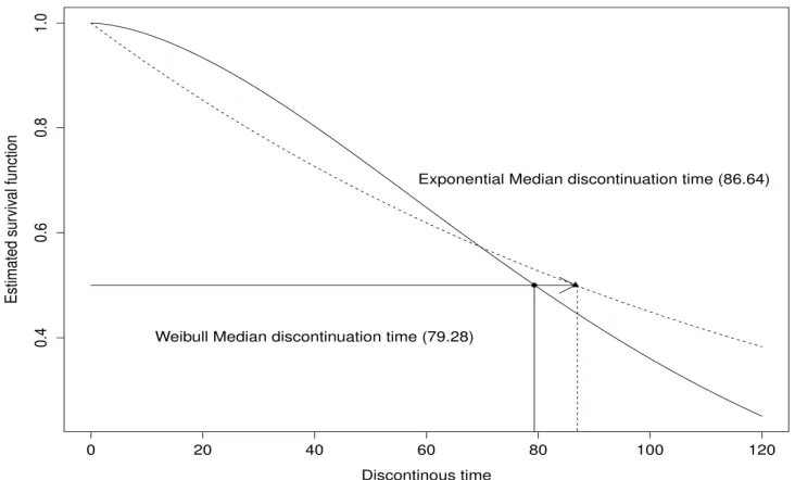
VII. CONCLUSION
In trials involving contraceptives, prevention of pregnancy is an obvious criterion for acceptability. The IUD data which was discussed in the whole chapter is the time origin corresponds to the first day in which woman uses IUD, and the end point is the discontinuation because of bleeding problems. Some women in the study ceased using IUD because of the desire of pregnancy, or because they had no further need for a contraceptive, while others were simply lost to follow-up. The data was fully analyzed in Bayesian framework.
Fig 5: Estimated survival curve for Weibull and exponential distribution showing their median survival time.
Weibull distribution, the estimated median discontinuation time for IUD data is 79.29 days and the 90 percentile is 162 days as reported in Figure 1. So 90%of women will have a discontinuation time less than 162 days. Hence it is very clear that the median is therefore estimated more precisely when the discontinuation time are assumed to have a Weibull distribution. It would also be evident from Table 7. Table 7 shows the deviance and DIC of both models. Here the deviance of Weibull model is 100 whereas exponential model have 207, which prove that Weibull model is suitable for this data and exponential model does not provide an acceptable fit to this data.
REFERENCES
1. R Development Core Team ,” R: A Language and Environment for Statistical Computing”, R Foundation for Statistical Computing, Vienna, Austria, ISBN 3-900051-07-0, URL http://www.R-project.org, 2015.
2. Statisticat, LLC, LaplacesDemon: “Complete environment for Bayesian Inference”, R package version 13.03.04, URL
http://www.bayesianinference. com, 2013.
3. J. A. Nelder, and R. Mead, “A simplex method for function minimization”, The Computer Journal Vol. 7, 308-313, 1965.
4. Y. Khan, and A. A. Khan, “Bayesian regression analysis of Weibull model with R and Bugs”, Statistical Methodologies and Applications, Vol. 2, 131-140, 2014.
5. Y. Khan, and A. A. Khan, “Bayesian analysis of Weibull and log normal survival models with censoring mechanism”, International Journal of Applied Mathematics, Vol. 26, 671-683, 2013.
6. Y. Khan, M. T. Alhtar, R. Shehla, and A. A. Khan, “Bayesian modelling of forestry data with R using optimization and simulation tools”, Journal of Applied Analysis and computation, Vol. 5, 38-51, 2015.
7. D. Collet, “Modelling Survival Data in Medical Research”, London: Chapman & Hall, 1994.
8. M. Puja, K. S. Puneet, R. S. Singh, and S. K. Upadhyay, “Bayesian Survival Analysis of Head and Neck Cancer Data Using Lognormal model”, Communications in Statistics-Simulation and computation, 2013.
9. L. Tierney, and J. B. Kadane, “Accurate approximations for posterior moments and marginal densities", Journal of the American Statistical Association, Vol. 81, 82-86, 1986.
10. L. Tierney, R. E. Kass, and J. B. Kadane, “Fully exponential Laplace approximations to expectations and variances of non-positive functions”, Journal of the American Statistical Association, Vol. 84, No. 407, pp. 710-716, 1989.
11. Erkanli, “Laplace approximations for posterior expectation when the model occurs at the boundary of the parameter space”, Journal of the American Statistical Association, Vol. 89, 205-258, 1994.
12. Ntzoufras, “Bayesian Modelling using WinBugs”, John Wiley & Sons, 2009