New Intelligent Classification Techniques for
Diagnosis of Diabetes Mellitus based on
Modified PSO
P.Palanikumar, M. Arun
Research Scholar, Dept of Electrical Engineering, Annamalai University, Chidambaram, India
Assistant Professor, Dept of Electrical Engineering, Annamalai University, Chidambaram, India
ABSTRACT: An overview of some of the classification techniques appearing in this paper for Diabetes diagnoses and treatment. Hybrid optimization techniques are in the form Artificial Neural networks, Genetic Algorithm, Fuzzy classifier, Support Vector Machine, Least Squares Support Vector Machine, Particle Swarm Optimization. All the techniques are analyzed using Pima Indians Diabetes Data set from UCI repository of machine learning databases. This review aims to conclude best optimization technique for Diabetes Mellitus Diagnosis
KEYWORDS: Diabetes Mellitus (DM), Artificial Neural networks (ANN), Genetic Algorithm (GA),Particle Swarm Optimization (PSO), Least Squares Support Vector Machine (LS-SVM).
I. INTRODUCTION
2 describes the problem background and related work. The proposed hybrid algorithm is introduced in section 3 while experimental results are presented in section 4. The last section is devoted to the conclusion and further research.
II. RELATED WORKS
In mathematics, computer science and operations research, mathematical optimization, also spelled mathematical optimization, alternatively named mathematical programming or simply optimization or optimization, is the selection of a best element (with regard to some criterion) from some set of available alternatives. In the simplest case, an optimization problem consists of maximizing or minimizing a real function by systematically choosing input values from within an allowed set and computing the value of the function. The generalization of optimization theory and techniques to other formulations comprises a large area of applied mathematics. More generally, optimization includes finding "best available" values of some objective function given a defined domain (or input), including a variety of different types of objective functions and different types of domains
2.1 Optimization Problem
An optimization problem can be represented in the following way: Given: a function f : A R from some set A to the real numbers Sought: an element x0 in A such that f(x0) ≤f(x) for all x in A ("minimization") or such that f(x0) ≥f(x) for all x in A ("maximization").Such a formulation is called an optimization problem Many real-world and theoretical problems may be modeled in this general framework. Problems formulated using this technique in the fields of physics and computer vision may refer to the technique as energy minimization, speaking of the value of the function f as representing the energy of the system being modeled.Typically, A is some subset of the Euclidean space Rn, often specified by a set of constraints, equalities or inequalities that the members of A have to satisfy. The domain A of f is called the search space or the choice set, while the elements of A are called candidate solutions or feasible solutions.The function f is called, variously, an objective function or cost function (minimization),[2] a utility function or fitness function (maximization), or, in certain fields, an energyfunction . A feasible solution that minimizes (or maximizes, if that is the goal) the objective function is called an optimal solution.
Linear programming (LP), a type of convex programming, studies the case in which the objective function f is linear and the constraints are specified using only linear equalities and inequalities. Such a set is called
a polyhedron or a polytope if it is bounded.
Nonlinear programming studies the general case in which the objective function or the constraints or both contain nonlinear parts. This may or may not be a convex program. In general, whether the program is convex affects the difficulty of solving it.
Quadratic programming allows the objective function to have quadratic terms, while the feasible set must be specified with linear equalities and inequalities. For specific forms of the quadratic term, this is a type of convex programming.
Stochastic programming studies the case in which some of the constraints or parameters depend on random variables.
2. Particle Swarm Optimization Algorithm
A basic variant of the PSO algorithm works by having a population (called a swarm) of candidate solutions (called particles). These particles are moved around in the search-space according to a few simple formulae.[8] The movements of the particles are guided by their own best known position in the search-space as well as the entire swarm's best known position. When improved positions are being discovered these will then come to guide the movements of the swarm. The process is repeated and by doing so it is hoped, but not guaranteed, that a satisfactory solution will eventually be discovered.Formally, let f: n→ be the cost function which must be minimized. The function takes a
a solution a for which f(a) ≤ f(b) for all b in the search-space, which would mean a is the global minimum. Maximization can be performed by considering the function h = -f instead.Let S be the number of particles in the swarm, each having a position xi∈ n in the search-space and a velocity vi∈ n. Let pi be the best known position of particle i and let g be the best known position of the entire swarm. A basic PSO algorithm is then
PSO is based on the principle that each solution can be represented as a particle in the swarm. Each particle has a position in the search space which is represented by a vector xi (xi1 , xi 2 ,..., xiD ) , where D is the dimensionality of the search space. Particles move in the search space to search for the optimal solutions. Therefore, each particle has a velocity which is represented as vi (vi1, vi 2,..., viD) ,during the movement, each particle updates its position and velocity according to its own experience and that of its neighbors. The best previous position of the particle is recorded as the personal best pbest, and the best position obtained by the population thus far is called gbest. Based on pbest and gbest, PSO searches for the optimal solutions by updating the velocity and the position of each particle according to the following equations:
x x v (1)
v vc1r1 ( pbest x) c2 r2 (gbest x) (2)
Where is inertia weight, which is to control the impact of the previous velocities on the current velocity. c1 and c2 are acceleration constants.r1 and r2 are random values uniformly distributed in [0,1]. The velocity is limited by a predefined maximum velocity,vmax and v [ vmax , vmax] The algorithm stops when a predefined criterion is met, which could be a good fitness value or a predefined maximum number of iterations. Inertia Weight plays an important role in the process of providing balance between investigation and manipulation. It determines the contribution rate of a particles previous velocity to its velocity at the current time step.The basic algorithm step can be explained in three stages which are described as follow, (i) Evaluating the fitness value of each particle. (ii) Updating local and global best fitness and positions. (iii) Updating the velocity and the position of each particle. The Pseudo Code of the Particle Swarm Optimization is shown below
The Pseudo Code of the Particle Swarm Optimization
Step1. Begin
Step2. randomly initialize particles swarm
Step3. while (the stopping criterion is not met)
Step4. evaluate fitness of particles
Step5. for n = 1 to number of particles
Step6. find pbest
Step7. find gbest
Step8. for d=1 to number of dimension of particle
Step9. update the position of particles by Eq. (1)-(2)
Step10. next d
Step11. next n
Step12. update the inertia weight value
Step13. next generation until stopping criterion is met
Step14. End
2.2 Least Squares Support Vector Machine
Least Squares Support Vector Machines (LS-SVM) are reformulations to the standard SVMs which lead to solving
emphasize and exploit primal-dual interpretations. Links between kernel versions of classical pattern recognition algorithms such as kernel Fisher discriminant analysis and extensions to unsupervised learning, recurrent networks and
control are available. Given a training dataset of N points { Xi , Yi }N i=1 ,with input data Xi Rn output Yi R , the optimization problem considering
mi n 〖J(w,b,e)=(/2) w^T w+(/2) ∑_(i=0)^n▒e^2 〗
(4)
Where is a regularization factor, e is the difference between the desired output and the actual output, and (.)is a nonlinear function mapping the data points into a high dimensional Hilbert space; in addition, the dot product in the high-dimensional space is equivalent to a
positive definite kernel function
(5)
In primal weight space, a linear classifier in the new space takes the following form Where W is the weight vector and b is
called as the bias term. bR. After elimination of w and e which generates the Support Vectori. (6)
Where Y=[Y1, Y2,……. YN ] ,=[ 1, 2……N] and Kernelmatrix is KRNxN The resulting estimated function is
(7)
Radial basis function RBF kernel is
(8)
The Pseudo Code of the Least Squares Support Vector Machine
Step 1: Load the training data set of n data points { Xi , Yi }N i=1 ,with input data Xi Rn output Yi R Step 2: Generate random weights for each input data point.
Step 3: Determine the value of the bias term b and initialize the error e for each point randomly. Step 4: Initialize and using random values.
Step 5: Search for values of e, w and b that minimize the objective function, (3) and, (4).
Step 6: Construct the Lagrangian function with the solution that must satisfy the KKT conditions in the set of, (5) Step 7: Calculate number of support vector s( ∝) using, (6)
Step 8: Training data for LS-SVM model could be classified using, (7) with RBF kernel function, (8) Step 9: Classify any new point by, (10) using RBF kernel function, (8)
Step 10: Loop until stopping criteria is met, usually until reach the maximum number of iterations.
III. PROPOSED WORK
A modified version of PSO was proposed, The main idea of this modified version is as in the following equations. For the ith particle in d dimension, it could update its velocity and position using,(9) and,(10)
x x v) (9) v vc1r1 ( pbest x) c2 r2 (gbest x)] (10)
where is a convergence factor, which can be calculated using following formula c-c2-4c (11)
Where c=c1+c2
In this proposed method is calculated using the formula (12)
Step 1: Initialize population of particles X(t) which consists of random positions x1, x2…. Xn and velocities V(t)are made up of the particle’s initial velocity v1, v2…… vn on ‘n’ dimensions.
Step 2: Evaluate the fitness for each particle.
Step 3: For each particle, find the maximum fitness and compare it to the best found so far (pbest), if f(xi) less then f(bbest) then f(bbestk)=xi
Step 4: Set Pi equals to the location of the maximum fitness value xi
Step 5: Compare fitness evaluation with the population’s overall previous best. If current value is better than gbest , then reset gbest to the current particle’s array index and value.
Step 6: Calculate the convergence factor using,(11) Step 7: Calculate the Inertia weight using,(12)
Step 8: Update the position of the particle according to, (9) and, (10) and the new population (+ 1) will be generated.
Step 9: Adjust the acceleration of the particles using,
Step 10: Loop to step (2) until stopping criterion is satisfied (Reach a maximum number of iterations )
A hybrid classification algorithm which integrates Modified-PSO algorithm as a parameters optimization technique and LS-SVM for classification was proposed The proposed algorithm for DM diagnosis and treatment is composed of two main stages, Parameters Optimization and Classification. Modified-PSO algorithm was used as a parameters
optimization technique aiming to improve the sitting of the parameter values of LS-SVM. Hence, overcoming it’s sensitivity to the parameter values changes. Classification stage using LS-SVM technique consists of two steps , Training followed by a Testing. The aim of parameters optimization stage using Modified-PSO is to find the optimal
values for the parameters of the LS-SVM classifier. The second stage utilizes LS-SVM to classify the DM patients into one of two classes (Live/Die) using the optimized parameters.
Algorithm-3: Proposed Algorithm:
Step 1: Load the data set of n data points, { Xi , Yi }N i=1 , where Xi is the input vector and YiR is the corresponding target with values {−1,+1}.
Step 2: Generate random weights for each input data point.
Step 3:Initialize the bias term b and the error e for each point randomly. Step 4: Find the optimal values for and using algorithm 1.
Step 5: Find optimal values of (e,w,b)for the objective function in, (3) and, (4). Step 6: Calculate number of support vectors (∝)using, (6)
Step 7: Classify any new point by using RBF kernel function, (8)
Step 8: Loop until stopping criteria is met, usually until reach the maximum number of iterations
IV. EXPERIMENTAL RESULTS
In this section, we present the performance evaluation methods used to evaluate the proposed method. Finally, we give the experimental results and discuss our observations from the obtained results. The proposed algorithm worked on Pima Indians Diabetes Data Set. Some of the records in this data set contains zeros in some features. Cells with zero entry were kept unchanged . The input for the Modified-PSO algorithm is total of 768 records. About 768 random individuals are generated in the search space for 100 Iterations. The output from the Modified-PSO is the optimal values for and , which are 100 and 0.5 respectively. LS-SVM classifier is run with the optimized parameters and RBF kernel function, (8), seeking to find the optimal hyper-plan that separates the search space into 2 classes (Live, Die) by finding the optimal values for (w, e and b) in the objective function, (3) and, (4) the classification accuracy was calculated using, (13)
True Negatives (TN): Classifies No Diabetic as No Diabetic. False Positives (FP): Classifies No Diabetic as Diabetic. False Negatives (FN): Classifies Diabetic as No Diabetic
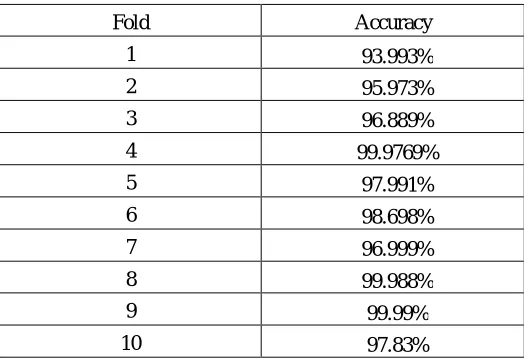
The performance of proposed method is evaluated using 10-fold cross-validation test. In this section, the obtained results are reported. The results with all features and optimal features found through modified PSO search in terms of Accuracy is shown in Table 1.
Fig(1) demonstrates the results of the average classification accuracy of the proposed algorithm against the accuracy of other classification algorithms applied on the same data set. Results show the effectiveness of the proposed Algorithm, which has the maximum average classification accuracy of 97.833% over other algorithms. TABLE(II) also articulates the average classification accuracy obtained from all algorithms in addition to the number of records used from Pima Indians Diabetes Data set in each algorithm
TABLE I. ACCURACY OF 10-FOLD CV
Fold Accuracy
1 93.993%
2 95.973%
3 96.889%
4 99.9769%
5 97.991%
6 98.698%
7 96.999%
8 99.988%
9 99.99%
10 97.83%
V. CONCLUSION AND FUTURE WORK
Diabetes is a complex and complicated disease characterized by either lack of insulin or a resistance to insulin, a hormone which is crucial for metabolism of blood sugar. This paper introduced a hybrid optimization Algorithm for DM patients. The proposed Algorithm integrates modified version of PSO and LS-SVM algorithm. The proposed algorithm was implemented on Pima Indians Diabetes Data set from UCI repository of machine learning databases. The average classification accuracy of LS-SVM method with RBF kernel was 97.833% which is the best while compared with other algorithms which worked on the same data set. As a future work, Ant Colony System (ACS) could be used as an optimization technique. Also, other kernel functions could be applied in the classification stage.
TABLE II. AVERAGECLASSIFICATIONACCURACY OF THE PROPOSED ALGORITHM AND OTHER CLASSIFCATION ALGORITHMS
Method Accuracy
GRNN 82.99%
Modified PSO fuzzy classifier 85.19 %
PSOANN 70.27%
Genetic Algorithm 80%
Fig. 1. Average Classification Accuracy of DM using the proposed algorithm and other classification algorithms
REFERENCES
[1] Centers for disease control and prevention, national diabetes, fact sheet, www.cdc.gov/diabetes (2011).
[2] World health organization, diabetes center, fact sheet n312,www.who.int/mediacentre/factsheets/fs312/en (2011). [3] http://ftp.ics.uci.edu/pub/ml-repos/machine-learning databases/pima-indians-diabetes, 2003.
[4] International Diabetes Federation 2011, Diabetes Atlas 4rd Edition, IDF
[5] Hamid Reza Sahebi,,Sara Ebrahimi “AFuzzy ClassifierBased on Modified Particle SwarmOptimizationfor DiabetesDisease Diagnosis” ACSIJ Advances in Computer Science: an International Journal, Vol. 4, Issue 3, No.15 , May 2015