On Network-based Control and Sensitivity Characterization of Mobile Robot in Intelligent Space

(1)

ABSTRACT

VANIJJIRATTIKHAN, RANGSARIT. On Network-Based Control and Sensitivity Characterization of Mobile Robot in Intelligent Space. (Under the direction of Dr. Mo-Yuen Chow.)

This dissertation addresses the problem of path-tracking control of a mobile robot, also

called an Unmanned Ground Vehicle (UGV), in Intelligent Space, where the controller is located on an entity different from the robot and communicates with the robot over a

communication network. The involvement of a communication network leads us to the core of this research, the network time-delay factor. The existence of a network delay presents a challenging problem that might degrade the overall system performance and even destabilize

the closed-loop control system.

The existing research area for the aforementioned scenario is called Network-based

control system (NBC) mostly focused on a general linear system for which the controller must be redesigned so that the overall NBC system can work properly. Distinct from the existing research, and innovative in its own right, the research presented in this dissertation

focuses on a specific nonlinear system, the remote UGV path-tracking. More specifically, we focus on the methods that allow the existing workable path-tracking controller to be reused in

the NBC environment.

In this work, Accumulated effect parameter tuning method is firstly proposed to tune the geometrical path-tracking controller used in UGV before operating over communication

network; then sensitivity analysis is introduced to consider how the system is sensitive to

(2)

processor (FP) is proposed to alleviate the effect of network delay by using UGV position estimation through UGV kinematics model; along with FP, UGV response time is proposed to demonstrate the effect of different UGV characteristics on path-tracking performance;

finally, the effect of using Gain scheduler (GS) with two-dimensional and one-dimensional gain table is investigated for the capability to alleviate the network delay on remote UGV

(3)

On Network-Based Control and Sensitivity Characterization of Mobile Robotin Intelligent Space

by

Rangsarit Vanijjirattikhan

A dissertation submitted to the Graduate Faculty of North Carolina State University

in partial fulfillment of the requirements for the Degree of

Doctor of Philosophy

Electrical Engineering

Raleigh, North Carolina 2008

APPROVED BY:

___________________________ ___________________________ Dr. Fen Wu Dr. Griff L. Bilbro

(4)

DEDICATION

To my parents, Phitaya and Sirima Vanijjirattikhan, and

my wife, Sukwida Manorangsan, for their endless love,

(5)

BIOGRAPHY

Rangsarit Vanijjirattikhan was born in Suphanburi, Thailand. He received his Bachelor

of Engineering in Computer Engineering from Kasetsart University, Bangkok, Thailand in 1996. He received his Master of Science in Electrical Engineering from North Carolina State

University in 2003. He is currently a Ph.D. candidate at North Carolina State University. During his study at North Carolina State University, he worked as a teaching assistant for a Mechatronics course. He also worked as a research assistant at Advanced Diagnosis,

Automation, and Control lab. His research area is in mobile robot path-tracking and Network-based control system. He is also interested in computer simulation and computer

(6)

ACKNOWLEDGEMENTS

I would like to express my deepest gratitude to Dr. Mo-Yuen Chow for his tireless effort

teaching me how to do research. Dr. Mo-Yuen Chow has been a great advisor with his care on many aspects of my student life. He also provided me an opportunity to come here to

study in USA. I am grateful to Dr. Chow and his kindness of providing me 5 years full financial support. I also would like to thank Dr. James J. Brickley, Dr. Griff L. Bilbro, and Dr. Fen Wu for his time being my committee and useful comments.

I would like to thank Dr. Yodyium Tipsuwan for his friendship and his help during my first two years in the USA. I thank my colleagues at Advanced Diagnosis, Automation, and

Control (ADAC) lab for their friendship and their help in several aspects of my study. I would like to make a special mention of Mr. Zheng Li for his insight on sensitivity research, Ms. Rachana A. Gupta for providing technical support at various stages, Mr. Manas Talukdar

for proof reading my dissertation, and making very insightful suggestions, Mr. Yixin Cai for contributing to the development of parts of the ADAC iSpace simulation program that I have been using, Mr. Lei Wang , Mr. Unnati Ojha, Ms. Preetika Kulshrestha and Mr. Hong-Bo Li

for several helpful comments on my oral exam presentation. I would like to thank my wife, Mrs. Sukwida Manorangsan, for being such a good friend and providing me supports on

every aspect of my life. I would like to thank my mother-in-law, Mrs. Siriporn Manorangsan, for her help in taking care of my son.

(7)

(8)

LIST OF TABLES

CHAPTER II

Table 1. * for VP path tracking... 36

0 d

Table 2. * for QC path tracking. ... 37

0 d

Table 3. * for PP path tracking. ... 37

0 d

Table 4. Tuned dmax and β... 38

Table 5. UGV parameters. ... 40

CHAPTER III

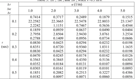
Table 1. Δτ , Δκ, and Δv when v=0.1 m/s. ... 67 Table 2. Δτ , Δκ, and Δv when v=0.2 m/s. ... 67 Table 3. Δτ , Δκ, and Δv, when v=0.3 m/s... 68

CHAPTER IV

Table 1. UGV chassis parameters... 85 Table 2. Motor parameters... 85

Table 3. Quadratic curve path tracking parameters. ... 86

CHAPTER V

(12)

Table 2. Motor parameters... 112

Table 3. Quadratic curve path-tracking parameters... 113

Table 4. Setups of the remote UGV path-tracking to be simulated... 118

Table 5. Path tracking cost for the simulation result set A. ... 121

Table 6. Path tracking cost for the simulation result set A with additional network delay. ... 121

Table 7. Path tracking cost for the simulation result set B. ... 122

(13)

LIST OF FIGURES

CHAPTER I

Fig. 1. Human-robot interaction in an iSpace... 5

Fig. 2. Intelligent Space. ... 6

Fig. 3. Local decision making in Control Agent... 7

Fig. 4. Global decision making in Control Agents. ... 8

Fig. 5. Simplified diagram of Network-based control system, Direct Structure. ... 10

Fig. 6. Distributed control system, Hierarchical Structure. ... 10

Fig. 7. Network-based control system. ... 11

Fig. 8. An example of feedback control system with network delay... 12

Fig. 9. Step responses of feedback control system with various network delay... 13

CHAPTER II Fig. 1. UGV path tracking using geometrical algorithm. ... 30

Fig. 2. UGV trajectory while using QC to track a constant curvature path with d0 = 0.5 m (left) and d0=0.4m (right)... 33

Fig. 3. UGV trajectory to illustrate the state representation. ... 35

(14)

Fig. 5. Area showing the distance the UGV moves caused by exerting the reference signal for one sampling step (left), Area showing the distance the UGV moves affected by the

UGV dynamics (right). ... 39

Fig. 6. Tracking path used in simulation. ... 40

Fig. 7. Path tracking cost according to different values of look-ahead distance (the dashed line is the tuned look-ahead distance)... 42

Fig. 8. Path tracking cost according to different values of look-ahead distance with added noise. ... 42

CHAPTER III Fig. 1. The overall structure of an iSpace. ... 51

Fig. 2. Network-based control system. ... 52

Fig. 3. Mobile robot path-tracking network-based control system... 55

Fig. 4. Information exchange between the mobile robot and the central controller. ... 57

Fig. 5. Path-tracking error without network delay... 59

Fig. 6. Path-tracking error with network delay τ . ... 59

Fig. 7. Path-tracking cost J (gray area) formed by robot trajectory... 61

Fig. 8. Path-tracking cost sensitivity respected to round trip time delay, _SJ τ . ... 64

Fig. 9. Path-tracking cost sensitivity respected to path curvature, _SJ κ ... 64

(15)

CHAPTER IV

Fig. 1. UGV path tracking network-based control system. ... 75

Fig. 2. Unmanned Ground Vehicle (UGV)... 78

Fig. 3. Conceptual diagram for quadratic curve algorithm... 79

Fig. 4. Timing diagram for data transmission between UGV and the controller. ... 81

Fig. 5. UGV path tracking NBC system applied with Feedback Preprocessor. ... 82

Fig. 6. The test path used for the time-delay effect analysis. ... 86

Fig. 7. The shortest distance between the UGV and the path... 87

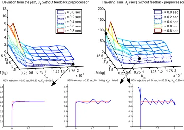
Fig. 8. Simulation Result, J1 and J2 (without Feedback Preprocessor). ... 88

Fig. 9. Simulation Result, J1 and J2 (with Feedback Preprocessor)... 89

Fig. 10. Step response of UGV wheel speed with response time T1, T2, T3 according to mass M= 1.5 kg and various motor electromotive force constants Km. ... 90

Fig. 11. UGV response time with various M and Km... 91

Fig. 12. J1 and J2 with respect to TUGV and τ. ... 91

Fig. 13. Contour plots of J1 and J2 with respect to TUGV and τ ... 92

CHAPTER V Fig. 1. Intelligent space in manufacturing plant. ... 99

Fig. 2. iSpace at NCSU prototype configuration. ... 100

Fig. 3. iSpace structure diagram. ... 102

Fig. 4. Main controller GUI program. ... 103

(16)

Fig. 6 Time diagram of the GSM operations. ... 107 Fig. 7. Remote mobile robot path-tracking model applied with GSM. ... 108 Fig. 8. The effect of the delay time on path-tracking mobile robot without FP (left) and

with FP (right)... 109 Fig. 9. Histogram of the random delay between ADAC lab and Hashimoto lab. ... 113

Fig. 10. 2-D gain for GS module. ... 114 Fig. 11. Scenario when the UGV tracks a straight path length l (left) and the distance ε that the UGV travels because of the adjusted speed (right)... 115

Fig. 12. 1-D gain table for GS module, on the left and on the right.

... 116

1

ˆ ( ki

new

K τ + ) ( )

new UGV

K κ

Fig. 13. Tracking path used in the simulation... 118 Fig. 14. The mobile robot while tracking the predefined path. ... 119 Fig. 15. Remote UGV path-tracking simulation result for set A when there is no delay,

when there is delay but without GSM, and when there is delay and GSM. ... 126 Fig. 16. Remote UGV path-tracking simulation result for set A with 0.35 sec additional

delay... 127 Fig. 17. Remote UGV path-tracking simulation result for set B when using GSM with 1-D

generated gain table having κ_UGV fixed at 0.0, 1.8573, and 11.5607 respectively... 128 Fig. 18. Remote UGV path-tracking simulation result for set C when using GSM with 1-D

generated gain table having τˆki+1 fixed at 210.0 msec, 236.9 msec, and 281.0 msec

(17)

APPENDIX A

Fig. 1. Unmanned Ground Vehicle (UGV)... 134 Fig. 2. Block diagram of the Unmanned Ground Vehicle (UGV)... 135

APPENDIX B

Fig. 1. Conceptual diagram for quadratic curve algorithm... 142

APPENDIX C

Fig. 1. Gain Scheduler Middleware for unmanned ground vehicle path-tracking. ... 147

(18)

CHAPTER I

INTRODUCTION

Automated Guided Vehicle (AGV) is usually referred to a mobile robot that can automatically move from one place to a desired place without the need for human intervention. There are several applications that emerge with the evolution of the AGV, such

as automated delivery system, patrol and security, and house hold application. AGV has gained much attention due to the need for efficient transportation[1], reducing human

workload, decreasing cost[2], and enhancing human life style[3]. Some examples of AGV in action are:

1. Fork Lift Vehicle (FLV) AGV from Egemin®[4] that can automatically move the

pallet for material handling task in several industries such as automotive, paper & printing, and textile.

2. Mobile robot from KIVA Systems®[5] that can automatically move product inventory in the distribution center such as WalGreens’ and Staple’s in order to facilitate online order fulfilment.

3. ADAM AGV from RMT Robotics®[6] used in the tire industry to transfer tires between work stations.

4. TransCar AGV from Swisslog®[7] used in hospital that can navigate through multi-floors facilities for material delivery.

(19)

Electrolux®[3], the autonomous vacuum cleaning robots that can do intelligence planning to traverse the floor area.

6. Automower from Husqvarna®, Robomower from Friendly Robotics®, and Lawnbott

from Zucchetti®[3], the autonomous robot that can automatically mow the lawn and come back to the dock station for battery charging without human interaction.

There are several research areas related with the algorithms that control the AGV such as artificial intelligence, path-planning, path-tracking, and collision avoidance ([8] and references therein, [9-11]). As the main purpose of the AGV is to be autonomous, the

controller that drives the robot is usually installed locally on the robot itself. This is distinct from the research area in our focus where the mobile robot is controlled by using

communication network for data exchange in the control loop. The aforementioned research area can be a basis for a new area of applications because, in several situations of mobile robot path-tracking control, the best decisions can be made from a remote site. For example,

in the situation where the AGV is tracking the path in a complex environment (such as a maze), the local sensors and controller on the AGV may not have enough information to guide the AGV to avoid obstruction and go to the destination. The sensors and controller

installed somewhere else, such as at the ceiling of the room, can acquire more useful information and guide the robot more efficiently. Or, in the situation that the controller

requires computing power such as interpreting human behavior by image processing, then the controller should locate on a computer with high computing power instead of on a small robot. The aforementioned situations are in line with a new application framework called

(20)

The research presented in this dissertation focuses on the problem of controlling a mobile robot to track a predefined path in which the exchanged data between the path-tracking controller and the mobile robot is conducted over a communication network. This

chapter introduces the motivation of our research including the challenge and the literature survey of the existing researches in the same area. This chapter is organized as follows:

Section I introduces the concept, structure, and advantage of an application area for remote UGV path-tracking called Intelligent Space; Section II introduces the network delay problem of Network-based control system; Section III provides a survey on the methods proposed for

network delay alleviation in NBC system. At the end of this chapter, we provide an outline of the rest of our dissertation.

I.INTELLIGENT SPACE

The existence of computational device and computer systems provide plenty of useful

applications such as robots in factory automation[13], computer numerical control milling machine in manufacturing process, automatic suspension control and anti-lock braking

system in automobiles[14], mower robot in household application[3], etc. However, current applications of computational devices are mostly limited by their physical location, i.e. the computational device is embedded into a local object such as the robots or cars.

A rapidly evolving and innovative trend in engineering research based applications is to spread computational devices including sensors and actuators into a space and to provide

(21)

Workspace or Intelligent Environment[12,15-17], as it has been called in published literature, is a novel way of providing the aforementioned services using autonomous agents with little or no human control effort involved. We will refer to such a system as iSpace. With advances

in technologies such as sensor network, network-based control, mechatronics, miniaturization of sensors and actuators (MEMS, NEMS), distributed control, robotics, etc., iSpace has been

rapidly evolving.

To demonstrate some general aspects of the systems mentioned above, system definitions from published literature are described here. In [12], Hashimoto defines

intelligent space (iSpace) as “a space where we can easily interact with computers and robots and get useful services from them”. In [16], NIST (National Institute of Standards and

Technology) defines Smart Space as “a work environment with embedded computers, information appliances, and multi-modal sensors allowing people to perform tasks efficiently by offering unprecedented levels of access to information and assistance from computers.”

And, in [17], Huang and Trivedi define Intelligent Environments as “systems that are aware of the spatial information and activities within them through sensors and interact with people in a natural and unobtrusive way.” All of these definitions emphasize on a natural way of

human-machine interaction and providing services according to human’s need.

As an example corresponding to the concept, Fig. 1 shows a room with a number of

(22)

Human

Webcam

Webcam Mobile Robot

Microphone Microphone

Webcam

Fig. 1. Human-robot interaction in an iSpace.

This scenario can be applied to a hospital where a patient is having difficulty helping

himself. If he is in iSpace, the patient can use verbal or posture command to ask the robots to help him get water and food, or allow the robots to take appropriate action in case of an

emergency.

In this manuscript, we adopt the iSpace architecture from the viewpoint of Hashimoto [12] because the structure that had been laid out is simple and covers all the major

functionalities of iSpace.

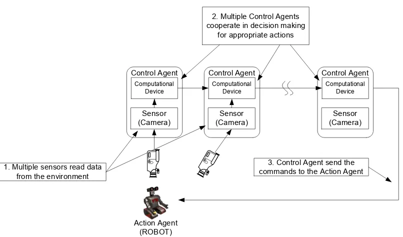
iSpace has 3 main types of components as shown in Fig. 2.

• Control Agent

• Communication Network

(23)

Action Agent

(ROBOT) HUMAN Action Agent(ROBOT)

Sens or

Comp utatio

nal

Devic

e _Sensor

Computational Device

Se nso_r

Co_mp uta

tion_al De

vice Communication Network

Physical Space Control Agent

Co ntro_{l A}

gen_t Contr

ol Ag ent

Fig. 2. Intelligent Space.

Control Agent composes of a computational device and sensors. The functionalities of

Control Agent are

• Observing events in the space via sensors such as camera, microphone, ultrasonic

sensors, etc.

• Processing data and transferring processed data to other Control Agents through

computer network in a sensor-independent format for further processing

• Making decisions according to the event observed by itself or by other Control

Agents on the network.

• Commanding the Action Agents, e.g. robots, to perform physical actions.

Communication Network (wired or wireless) is used to transfer data among Control

Agents and Action Agents.

(24)

is to execute tasks to support people in the physical space.

In order to provide a service, Control Agents in iSpace make (1) local decisions based on it’s own sensor information or

(2) global decisions based on aggregated information from other Control Agents (collaborative decision and control) as shown in Fig. 3 and Fig. 4 respectively.

As a result, Control Agents can compute distributively when compared to an integrated computational device.

Sensor (Camera)

Control Agent

1. Sensor read data from the environment 2. Control Agent makes decision for appropriate actions based on local

computational device

3. Control Agent send the commands to the Action Agent

Action Agent (ROBOT)

(25)

Sensor (Camera)

Control Agent

1. Multiple sensors read data from the environment

2. Multiple Control Agents cooperate in decision making

for appropriate actions

3. Control Agent send the commands to the Action Agent

Action Agent (ROBOT)

Sensor (Camera)

Control Agent

Sensor (Camera)

Control Agent

Fig. 4. Global decision making in Control Agents.

Many different research areas such as human-machine interface, human position prediction, face recognition, omnivision sensors, and robot navigation[17-20] are currently involved in investigating and developing iSpace. There are still many issues and open

problems that need much more investigation. One important research topic that arises in iSpace is to solve the network delay problem that occurs when remote controllers (control

agents) send control signals to the actuators (action agents) through a communication network.

In general, integration/collaboration among computational device, sensors, and actuators

to offer a service starts from sensors getting data from the environment. Then, the data is transferred to the computational device for processing and collecting useful information.

(26)

command/reference signal is sent between computational device, sensors, and actuators. As a result, the actuators’ performance (e.g., accuracy, stability, robustness) might degrade. One reason for the performance degradation is the time shift where the actuators receive a control

command that is not appropriate for the current time period.

We can formulate this network delay issue in the iSpace as a closed-loop control system

operated over a communication network. In the next section, we introduce the problem of control performance degradation that may be caused by network delay.

II.NETWORK-BASED CONTROL SYSTEM AND NETWORK DELAY PROBLEM

Control system can be classified as open-loop control system or closed-loop control

system (feedback control system). In general, open-loop control system refers to the control system where the controller ignores the outcome of the controlled process. The controller only uses the signal from the reference input r to determine the control signal u. On the other

hand, closed-loop control system or feedback control system refers to the control system that the controller can observe the result of the controlled process (controlled variable, y) in

addition to only the objective (reference input, r) available in open-loop control system. For conventional feedback control system, data transfer between controller and controlled process is direct and immediate. But, in some cases, the connection between

controller and controlled process is implemented by a communication network. This can introduce several advantages to the control applications such as reducing investment and

maintenance cost for wiring complexity (e.g., in factory automation), enabling teleoperation, and rendering new control concepts and applications [12,16,21-23].

(27)

communication within a single computer to global and massive information sharing over the Internet. Communication networks also take part in control system applications such as the control network in automobiles, teleoperation of robot arm manipulators, and distributed

control of multiple robots [21,24,25]. This network-based control (NBC) system, networked control system (NCS), or distributed control system [26-28] is an emerging topic that has

gained a lot of attention during the last decade.

N

There are several structures for the NBC system implementation. Denoting controller by

Cn, sensor by Sn, and actuator by An, n=1, 2, ,… , a control system with communication

network can be configured in a Direct Structure as shown in Fig. 5, or in a Hierarchical

Structure as shown in Fig. 6.

S₁ A₁

C₁ Network Control signal

Sensor measurement

Fig. 5. Simplified diagram of Network-based control system, Direct Structure.

S₁ A1

C₁

S₂ A2

C₂

S₃ A3

C₃

C_M

S₁ A1

C₁

S₂ A2

C₂

S₃ A3

C₃

C_M

Network

Fig. 6. Distributed control system, Hierarchical Structure.

(28)

of the subsystems. An example of the cooperation is that Cm provides reference inputs to C1,

C2, and C3 while C1, C2, and C3 control their own actuator according to the received

reference input. Because the components of the control system in both Fig. 5 and Fig. 6 are

physically decentralized, we also call these kind of systems as distributed control system [29].

In this dissertation, we will focus only on the direct structure which can be represented by the block diagram shown in Fig. 7.

CONTROLLER

Control

signal, u CONTROLLED

PROCESS

Controlled variable, y

COMMUNICATION NETWORK, Nt

Reference input, r

+ _

Error, e

SENSOR

Fig. 7. Network-based control system.

The sequence of operation for network-based control (NBC) system starts from the

controller generating control signal (u), from the error (e) between reference input (r) and controlled variable (y) (Fig. 7). The control signal u is sent through the communication

network Nt to actuate the controlled process or actuator. According to the system dynamics,

the output of controlled process is generated, measured by sensor, and then, sent back to the controller to complete the process cycle. The controller then starts to generate a control

signal and sends it to the actuator for the next cycle. Studies show that the network delay induced by the communication network can degrade the performance and reduce the stability

(29)

We simulate a NBC system composed of an actuator/plant, a controller and communication delays as shown in Fig. 8. The plant is a third-order system described by a

transfer function ( ) 30 ( 3)( 6)

G s

s s s

=

+ + . The controller is a proportional controller with gain

of one. The reference signal of the feedback control loop is provided by a step function.

Fig. 8. An example of feedback control system with network delay.

The simulation results of the step response with various constant delays are depicted in Fig. 9. These results demonstrate that increasing delay time also increases the system overshoot and settling time. Hence, the system performance is degraded as the delay time is

(30)

Fig. 9. Step responses of feedback control system with various network delay.

The simulation results in Fig. 9 show that it is important to have the effect of network delay considered when designing a NBC system. In the next section, a survey on existing

literature that had been proposed to alleviate the effect of network delay is presented.

III.SURVEY ON NBC SYSTEM

Control applications using communication networks can reduce investment and maintenance cost for wiring complexity (e.g., in factory automation), and render new control

concepts and applications such as iSpace[12,18,39-41]. One major area of application of a control system with network is teleoperation, such as the Jason project[42] with an undersea

robot exploring the famous sunken ship Titanic, the Mercury project[23] with the first on-line robotics arm to explore the terrestrial surfaces, the Xavier project[43] with the first on-line mobile robot moving to a destination preset by the remote user, the USAR (Urban Search

(31)

minimal invasive surgery, and NASA’s Mars Exploration Rovers[22] with the ability to survey Martian terrain.

Among all the control systems with network, one major challenge is the existence of a

network delay that might degrade the overall system performance and even destabilize the closed-loop control system in the network.

There exist several approaches to alleviate the effect of delay time. As in teleoperation where the human operator can use a master robot to remotely control a slave robot located far away, the simplest method is to use human intuitive to learn about the effect of network

delay and perform “move and wait”, in which the operator slightly moves the master robot at a time [45]. Then, the operator waits to observe the slave robot to see if the movement is

under control. In this way, the operator can get some knowledge of the delay effect and be able to control the master robot to the extent that the slave robot is still working as expected. Another method to deal with the network delay is “teleprogramming” where there exists an

extra controller at the remote plant as shown by the hierarchical structure in Fig. 6 [46]. The central controller (human or a program) needs to send only a command or a task to the remote plant. Then, that extra controller will take responsibility to finish the task and network

delay will not have any effect on this local operation. This method presents a solution of the communication delay problem in a system in which the delay does not need to be directly

considered. As a result, the system tends to be less flexible and less interactive compared to the system that directly uses the information of the delay time and has the feedback loop span over the communication network. This aspect is the primary focus of the research presented

(32)

One well-known direction in dealing with communication delay in NBC is by using passivity theorem. Along this line, Anderson and Spong [31] used the power variable in force feedback teleoperation to successfully stabilize the NBC system in passive environment

under an arbitrary size of the delay. Niemeyer and Slotine [47] introduced the wave variable instead of power variable for information exchange in force feedback teleoperation. In

addition to robustness and system stability to arbitrary network delay, wave variable has the benefit to reduce the complexity of the system implementation. In [33,48], Hannaford and Ryu harnessed the concept of passivity to enhance the haptic interface system which has the

information flow in two directions, like force feedback teleoperation system. They used a real-time energy measurement module and adaptive energy dissipative element in order to

interactively control the net energy of the system so that the stability of the system is achieved with less conservative than a rigid passivity based design.

Another direction to address the NBC problem is focusing at the communication

network to derive a suitable network characteristic such as the communication protocol, scheduling algorithm, transmission rate, and bandwidth. In [32,49] Halevi and Ray proposed an analytical technique to test the stability of a specific NBC system whose communication

delay can be assumed periodic. Their approach can be applied to a token passing network, such as token ring. They also proposed a time skew varying method to reduce the vacant

sampling and message rejection of the data packet transmitted between the controller and the plant through a communication network. This method will help the controller to have higher probability of getting the most updated data from the sensor and eventually improve the

(33)

try-once-discard (TOD), for multiple-input-multiple-output (MIMO) NBC system. TOD allows the node that has the highest priority to get the transmission while ensuring the maximum allowable transfer interval of every node to guarantee stability. In [34], Zhang et al. studied

the relationship between the network round-trip-time delay (RTT), controller sampling period, and the stability of a system. They proposed an analytical method to find a stability

region given controller sampling period and RTT for a specific case of the system. Their results also include the stability condition of a NBC hybrid system, system with packet dropouts, and multiple-packet transmission. In [28] Lian et al., proposed a guideline to find a

relationship between the control quality of performance (QoP) and the network and control parameters. They provided a method to choose a proper sampling period so that the rate of

the data exchange between the controller and the plant is high enough to maintain an acceptable performance but not too high until the network is congested.

Another direction to deal with network delay in NBC system is by using techniques

based on soft computing such as Neural network and Fuzzy logic. In [38] Almutairi et al. uses fuzzy logic compensation method to compensate network delay effect by externally updated PI controller gain with respect to the system output error caused by network delay.

In [50], Lee et al. proposed the remote fuzzy logic controller method in which a typical PID controller is replaced by a fuzzy logic controller. For both methods, the expert knowledge

can be embedded within the fuzzy rules to calculate the control signal based on the system error in order to alleviate the effect of delay. On the other hand, Neural network (NN) does not need the expert knowledge but uses learning capability to cope with the delay effect. In

(34)

system control under constant delay. Smith predictor is a famous method to control a system with delay using an accurate model-based prediction [52]. Huang and Lewis propose to use recurrent neural network to compensate the nonlinear effect of the plant so that the plant can

be treated as a linear system to be controlled using Smith predictor.

Several researchers approached the network delay problem by considering model-based

predictor. In [53], Luck and Ray use observer-based compensator to alleviate the effect of network delay. They use observer to determine the state of the plant from the plant output. Then, based on the plant model, the compensator can estimate the current plant state from the

delayed plant state so that the controller will get the most updated state to calculate the control signal. In [54], Chan and Ozguner used the estimated state of the plant based on the

transmission queue length information embedded in the data packet before sending it from the plant. The queue length can determine how many time periods have passed after the plant output is measured. Then, a model-based predictor can predict the state of the plant so that

the control signal can be prepared accordingly. In [37], Montestruque and Antsaklis use model-based prediction to predict the future state of the linear plant. A stability condition is also provided so that the maximum period of two consecutive data transmissions can be

determined to reduce the network load while the system remains stable.

The stability of the NBC system is also studied using the counterpart of the Lyapunov

stability condition, Lyapunov-Krasovskii and Razumikhin stability condition. There is emerging literature focussing in this direction such as [36,55] and the references therein. For a linear NBC system in general, the stability can be tested by formulating the L-K or

(35)

represented by Linear Matrix Inequalities which can be efficiently solved by existing algorithm [56].

Optimal stochastic control and robust control have also been reported to have the

capability to alleviate the network delay problem. In [35], Nilsson proposed an optimal stochastic control method to control a NBC system in which the random round-trip-time

delay is less than the sensor sampling period. This method can derive an optimal control signal subjected to minimizing a predefined cost function. In [57], Shousong and Qixin formulate a NBC system so that the optimal stochastic control framework can be applied to

the NBC system where the delay time is larger than the controller sampling period. In [58,59], robust control framework is used to alleviate the effect of delay time. Random delay

is treated as bounded system uncertainties and the robust controller is designed for all system variation under uncertainties to ensure a predefined limit of the error amplification (i.e., the plant output can track the reference signal within a bound). In [60], Kyoo Kim et al.

formulate a NBC system into several patterns according to the history of the delay. Several

controllers are designed to form a switched

H_∞ H_∞ controller in order to ensure a bounded

error amplification corresponding to the pattern of the delay history for each time instant. The aforementioned researches mostly focus on a general linear system for which the controller must be redesigned so that the overall NBC system can work properly. Distinct

from the existing research, and innovative in its own right, the research presented in this dissertation focuses on a specific nonlinear system, the remote UGV path-tracking. More

(36)

into the existing system so that the outputs from the UGV is preprocessed before using them in the control signal calculation and the control signals are adjusted appropriately for current network traffic condition and path-tracking environment.

The succeeding chapters are organized as follows. In chapter II, we focus on the parameters tuning of path-tracking algorithm as it is important that the path-tracking

parameters should be finely tuned before operating in NBC environment.Chapter III focuses on how the path-tracking error is sensitive to the UGV speed, path curvature, and magnitude of network delay so that we can carefully compensate when those signals have noise or

perturbation. Chapter IV focuses on the Feedback Preprocessor module to preprocess the sampled data from the UGV before using them in path-tracking controller in order to

alleviate the effect of network delay. Chapter IV introduces the concept of UGV response time to predict the level of performance degradation caused by network delay. Finally, Chapter V focuses on applying Gain Scheduler Middleware with a variation of gain table to

alleviate the effect of network delay in Intelligent Space by externally adjusting the path-tracking controller gain.

REFERENCES

[1] J. Zhang, P. A. Ioannou, and A. Chassiakos, "Automated container transport system between inland port and terminals," ACM Transactions on Modeling and Computer Simulation (TOMACS), vol. 16, pp. 95-118, 2006.

[2] P. A. Ioannou, et al., "Advanced Material Handling: Automated Guided Vehicles in Agile Ports," Center for Advanced Transportation Technologies, Univ. Southern California, Los Angeles, 2000.

(37)

[4] http://www.egeminusa.com/.

[5] http://www.kivasystems.com/. [6] http://www.adam-i-agv.com/. [7] http://www.swisslog.com/.

[8] I. F. A. Vis, "Survey of research in the design and control of automated guided vehicle systems," European Journal of Operational Research, vol. 170, pp. 677-709, 2006.

[9] K. Yoshizawa, et al., "Path tracking control of mobile robots using a quadratic curve," Proceedings of the 1996 IEEE Intelligent Vehicles Symposium, 1996.

[10] O. Amidi, "Integrated Mobile Robot Control, tech. report CMU-RI-TR-90-17," Robotics Institute, Carnegie Mellon University 1990.

[11] J. Wit, C. D. Crane III, and D. Armstrong, "Autonomous ground vehicle path tracking," Journal of Robotic Systems, vol. 21, pp. 439-449, 2004.

[12] H. Hashimoto, "Intelligent space - How to make spaces intelligent by using DIND?," Proceedings of the 2002 IEEE International Conference on Systems, Man and

Cybernetics, Yasmine Hammamet, Tunisia, 2002.

[13] M. Mes, M. van der Heijden, and J. van Hillegersberg, "Design choices for agent-based control of AGVs in the dough making process," Decision Support Systems, vol. 44, pp. 983-999, 2008.

[14] R. Isermann, R. Schwarz, and S. Stolzl, "Fault-tolerant drive-by-wire systems," IEEE Control Systems Magazine, vol. 22, pp. 64-81, 2002.

[15] B. F. Johanson, A.; Winograd, T., "The Interactive Workspaces project: experiences with ubiquitous computing rooms," Pervasive Computing, IEEE, vol. 1, pp. 67-74, 2002.

(38)

[17] K. S. Huang and M. M. Trivedi, "Networked omnivision arrays for intelligent environment," Proceedings of Applications and Science of Neural Networks, Fuzzy Systems, and Evolutionary Computation IV, San Diego, CA, 2001.

[18] P. T. Szemes, T. Sasaki, and H. Hashimoto, "Mobile agent in the intelligent space which can learn human walking behavior," Proceedings of the 2005 IEEE/ASME International Conference on Advanced Intelligent Mechatronics, 2005.

[19] S. K. Das, et al., "The role of prediction algorithms in the MavHome smart home architecture," IEEE Wireless Communications, vol. 9, pp. 77-84, 2002.

[20] K. Morioka, et al., "Robust tracking of multiple objects using color histogram in intelligent environment," Proceedings of the 2003 IEEE/ASME International Conference on Advanced Intelligent Mechatronics, 2003.

[21] J. Leven, et al., "DaVinci Canvas: A Telerobotic Surgical System with Integrated, Robot-Assisted, Laparoscopic Ultrasound Capability," in Medical Image Computing and Computer-Assisted Intervention (MICCAI), 2005, pp. 811-818.

[22] J. J. Biesiadecki, P. C. Leger, and M. W. Maimone, "Tradeoffs Between Directed and Autonomous Driving on the Mars Exploration Rovers," The International Journal of Robotics Research, vol. 26, pp. 91-104, 2007.

[23] K. Goldberg and R. Siegwart, Beyond webcams : an introduction to online robots. Cambridge, MA: MIT Press, 2002.

[24] N. Navet, et al., "Trends in Automotive Communication Systems," Proceedings of the IEEE, vol. 93, pp. 1204-1223, 2005.

[25] A. Al-Jumaily and S. Kozak, "Behavior based multi robot cooperation by target/task negotiation," Proceedings of the 2004 IEEE Conference on Robotics, Automation and Mechatronics, 2004.

[26] Y. Tipsuwan and M.-Y. Chow, "Control Methodologies in Networked Control Systems," Control Engineering Practice, vol. 11, pp. 1099-1111, 2003.

[27] G. C. Walsh and H. Ye, "Scheduling of networked control systems," in IEEE Control Systems Magazine, vol. 21, 2001, pp. 57-65.

(39)

[29] R. Uusijävri and M. Törngren, "Introducing Distributed Control in Mobile Machines Based on Hydraulic Actuators," Journal of Mechatronics, vol. 4, pp. 139-157, 1994.

[30] G. C. Walsh, H. Ye, and L. G. Bushnell, "Stability analysis of networked control systems," IEEE Transactions on Control Systems Technology, vol. 10, pp. 438-446, 2002.

[31] R. J. Anderson and M. W. Spong, "Bilateral control of teleoperators with time delay.," IEEE Transactions on Automatic Control, vol. 34, pp. 494-501, 1989.

[32] Y. Halevi and A. Ray, "Integrated communication and control systems : Part I - Analysis," Journal of Dynamic Systems, Measurement, and Control, vol. 110, pp. 367-373, 1988.

[33] B. Hannaford and J.-H. Ryu, "Time-domain passivity control of haptic interfaces,"

IEEE Transactions on Robotics and Automation, vol. 18, pp. 1-10, 2002. [34] W. Zhang, M. S. Branicky, and S. M. Phillips, "Stability of networked control

systems," IEEE Control Systems Magazine, vol. 21, pp. 84-99, 2001.

[35] J. Nilsson, "Real-time control systems with delays," in Department of Automatic Control. Lund, Sweden: Lund Institute of Technology, 1998, pp. 138.

[36] K. Gu, V. Kharitonov, and J. Chen, Stability of time-delay systems. Boston [Mass.]: Birkhèauser, 2003.

[37] L. A. Montestruque and P. J. Antsaklis, "On the model-based control of networked systems," Automatica, vol. 39, pp. 1837-1843, 2003.

[38] N. B. Almutairi and M.-Y. Chow, "Stabilization of Networked PI Control System Using Fuzzy Logic Modulation," Proceedings of the American Control Conference, Denver, Colorado, 2003.

[39] W.-L. Leung, et al., "Intelligent space with time sensitive applications," Proceedings of the 2005 IEEE/ASME International Conference on Advanced Intelligent

Mechatronics, Monterey, California USA, 2005.

[40] J.-H. Lee and H. Hashimoto, "Intelligent Space - Its concept and contents," Advanced Robotics Journal, vol. 16, pp. 265-280, 2002.

[41] R. Vanijjirattikhan, et al., "Mobile Agent Gain Scheduler Control in Inter-Continental Intelligent Space," Proceedings of the 2005 IEEE International Conference on

(40)

[42] http://www.jasonproject.org/.

[43] R. Simmons, et al., "Lessons learned from Xavier," IEEE Robotics & Automation Magazine, vol. 7, pp. 33-39, 2000.

[44] R. R. Murphy, "Human-robot interaction in rescue robotics," IEEE Transactions on Systems, Man, and Cybernetics, Part C: Applications and Reviews, vol. 34, pp. 138-153, 2004.

[45] T. B. Sheridan, "Space teleoperation through time delay: review and prognosis,"

Robotics and Automation, IEEE Transactions on, vol. 9, pp. 592-606, 1993.

[46] J. Funda, T. S. Lindsay, and R. P. Paul, "Teleprogramming: toward delay-invariant remote manipulation," Presence: Teleoperators and Virtual Environments, vol. 1, pp. 29-44, 1992.

[47] G. Niemeyer and J.-J. E. Slotine, "Telemanipulation with Time Delays," The International Journal of Robotics Research, vol. 23, pp. 873-890, 2004.

[48] J.-H. Ryu, D.-S. Kwon, and B. Hannaford, "Stable teleoperation with time-domain passivity control," IEEE Transactions on Robotics and Automation, vol. 20, pp. 365-373, 2004.

[49] A. Ray and Y. Halevi, "Intergrated communication and control systems: Part II - Design considerations," Journal of Dynamic Systems, Measurement, and Control, vol. 110, pp. 374-381, 1988.

[50] S. Lee, S. H. Lee, and K. C. Lee, "Remote fuzzy logic control for networked control system," Proceedings of the 27th Annual Conference of the IEEE Industrial

Electronics Society (IECON '01), 2001.

[51] J.-Q. Huang and F. L. Lewis, "Neural-network predictive control for nonlinear dynamic systems with time-delay," IEEE Transactions on Neural Networks, vol. 14, pp. 377-389, 2003.

[52] O. J. M. Smith, "A controller to overcome dead-time," Instrument Society of America Journal, vol. 6, pp. 28-33, 1959.

[53] R. Luck and A. Ray, "An observer-based compensator for distributed delays,"

(41)

[54] H. Chan and U. Ozguner, "Closed-loop control of systems over a communications network with queues," International Journal of Control, vol. 62, pp. 493-510, 1995.

[55] E. Fridman, "New Lyapunov-Krasovskii functionals for stability of linear retarded and neutral type systems," Systems & Control Letters, vol. 43, pp. 309-319, 2001.

[56] S. P. Boyd, Linear matrix inequalities in system and control theory. Philadelphia: Society for Industrial and Applied Mathematics, 1994.

[57] H. Shousong and Z. Qixin, "Stochastic optimal control and analysis of stability of networked control systems with long delay," Automatica, vol. 39, pp. 1877-1884, 2003.

[58] G. M. H. Leung, B. A. Francis, and J. Apkarian, "Bilateral controller for teleoperators with time delay via mu-synthesis," IEEE Transactions on Robotics and Automation, vol. 11, pp. 105-116, 1995.

[59] F. Goktas, J. M. Smith, and R. Bajcsy, "mu-synthesis for distributed control systems with network-induced delays," Proceedings of the 35th IEEE Decision and Control, 1996.

(42)

CHAPTER II

ACCUMULATED EFFECT PARAMETER TUNING METHOD

FOR GEOMETRICAL PATH TRACKING OF WHEELED

MOBILE ROBOTS

Rangsarit Vanijjirattikhan, Manas Talukdar, Mo-Yuen Chow

rvanijj, mtalukd, [email protected]

Advanced Diagnosis Automation and Control Lab

Department of Electrical and Computer Engineering North Carolina State University, Raleigh NC 27695, USA

This chapter is published in the proceedings of the 2007 IEEE/ASME International

(43)

ACCUMULATED EFFECT PARAMETER TUNING METHOD

FOR GEOMETRICAL PATH TRACKING OF WHEELED

MOBILE ROBOTS

Abstract - This paper proposes a novel method for parameter tuning in geometrical path

tracking algorithms for wheeled mobile robots. Geometrical path tracking has the advantage in its ease of implementation. However, before using such an algorithm, several critical parameters need to be found experimentally. Such a procedure is quite time consuming and

unreliable. Moreover, there is no certainty that the parameters found using this method will hold for different kinds of paths. The research presented in this paper addresses this

particular issue. A tuning method called Accumulated Effect (AE) parameter tuning method is proposed for determining the appropriate parameter values which will hold for different paths under different conditions. This method is based on the steady state of a mobile robot,

tracking a circular path. The effectiveness of this method has been demonstrated using simulation results for three different path tracking algorithms.

Keywords: mobile robot, parameter tuning, path tracking

I. INTRODUCTION

Path tracking of wheeled mobile robot has gained substantial research attention in last

decade due to extensive applications of wheeled mobile robot such as automatic inventory

(44)

Network-based control applications [3, 4].

There are three basic problems related with the path tracking of wheeled mobile robot. We can categorize the existing literature based on these three problems:

• The first problem is path following where there exists a path known by the

controller and the mobile robot needs to follow the path.

• The second problem is trajectory tracking where there exists a virtual reference

robot moving along the desired path and the actual mobile robot needs to be

controlled to converge to the reference robot.

• The third problem is set point stabilization where there exists a final posture

where the robot at an initial posture is required to converge to.

Ideally, a path tracking algorithm should address all of these problems. Most existing

algorithms address one or a combination of these problems. Some existing works are geometry based path tracking controller proposed by Amidi [5], Yoshizawa [6], and Wit [7],

which can address the path following problem and the trajectory tracking problem. The kinematics model based stable non-linear path tracking controller proposed by Kanayama et al. [8] and adaptive fuzzy logic-based controller by Das and Kar [9], addresses the trajectory

tracking problem. Globally stabilizing time-varying feedback approach proposed by Samson [10] and dynamic feedback linearization approach proposed by Oriolo et al. [11], addresses

both the trajectory tracking and set point stabilization. Robust adaptive controller based on neural network and backstepping paradigm by Fierro and Lewis [12], addresses all of the problems. Each of these approaches has their own nuances. For example, [8, 10, 11] consider

(45)

the kinematics and dynamics for controller design. [9, 12] also has the capability to adapt the controller based on model uncertainty. [5, 6] considers only the position error between the robot and the path/trajectory while the other algorithms also consider the heading error.

In this paper, we focus on the path following problem implemented by geometrical algorithms [5-7]. These algorithms are relatively easy to implement after the information of

the path is known since there is no need to generate the trajectory of the virtual reference robot as aforementioned in the trajectory tracking problem. However, using these geometrical algorithms require tuning of some parameters which are typically done by

experiment and can be time consuming. Therefore, we propose a parameter tuning method called Accumulated effect (AE) parameter tuning approach based on the numerical result of

the steady state, while the robot tracks a constant circular path. A bound of path deviation error is used in the tuning process so that the robot using the tuned parameter has path-deviation error approximately within the assigned bound.

The parameter tuning for geometrical path tracking is a vital issue which merits meticulous research. There is an existing work [13] that addresses the look-ahead distance for a stable pure pursuit path tracking system. However, there is no analysis on the path tracking

performance. Some other literature [9, 12] address the issue of the unknown robot dynamics parameter, but up to our awareness, there has been no specific detailed study of geometrical

path tracking parameter tuning.

This paper is organized as follows: in section II, the system setup is described, section III discusses the parameter tuning method of geometrical path tracking algorithm, section IV

(46)

II.SYSTEM SETUP

In this section, we give an overview of the unmanned ground vehicle (UGV) path

tracking system used in this research. The focus here will be on path following problem where the path can be varied according to the environment and the information of the path is

known by the path tracking controller (e.g., UGV for services in hospitals, offices, homes, or industrial plants [2]).

A. Uumanned ground vehicle model

In this research, we considered the path tracking of a differential drive mobile robot with two driving wheel and one or more caster wheels. The UGV can turn by driving the wheels

with two different speeds. The center of turn is treated as the point-wise position of the UGV for path tracking error calculation. The center of turn can be different from the center of gravity (CG) because the position of the wheel may be away from the most density part of

the mass.

]

The model of the UGV is used to describe the behavior of the UGV according to the

control signal which is reference speed and turn rate, u . This UGV model is

composed of the UGV kinematics & dynamics, the motor dynamics, and the motor speed controllers. The simulation in this paper is based on the nonholonomic UGV kinematics &

dynamics described in [14] and the DC motor and gear train model described in [15]. [v_refω_ref T

=

B. Path tracking algorithms

(47)

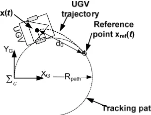
drive the UGV along a predefined path.

In order to track the path, the UGV needs to target one reference point on the path at a

time and steer towards that point. The reference point will lead the

UGV and keep a distance, called look-ahead distance (d0), ahead of the UGV as shown in

Fig. 1. As the UGV follows the reference point and the point moves along the path, the UGV eventually tracks the predefined path.

( ) [ ]T

ref t = xref yref

x

G

Σ

Fig. 1. UGV path tracking using geometrical algorithm.

d0 can be a fixed constant as in PP and VP or a function of the tracking condition as in

QC. In QC, the look-ahead distance is adjusted based on the curvature of the path, using the

quadratic coefficient (A), as calculated by Eqn. (1) where dmax and β are constants, A is

equal to 1 2R_UGV .

0 max (1 )

d = d +β A ₍₁₎

For all three algorithms, after the path tracking controller knows where the reference point in each calculation step is, the UGV needs to find the speed gain K and the circular radius of the UGV trajectory RUGV in order to calculate vref and ωref according to Eqn. (2)-(3)

ref

(48)

UGV

ref K R

ω = ₍₃₎

where v_ref is the speed of the UGV in m/s and ω_ref is the turn rate of the UGV describing

how the heading angle changes in rad/s. By using the control signal from Eqn. (2)-(3), the

UGV will run along a circle path radius RUGV with the speed K m/s. In VP and PP, is

typically kept constant. However, in QC, is changed according to the path curvature as

shown in Eqn. (4)

ref v

( )x (1 )

ref

v =sign e α + A (4)

where α is a constant, sign e( )_x is 1 if the reference point is ahead of the UGV and -1 if it is

behind the UGV. For the detailed calculation of K and RUGV for VP, QC, and PP, please refer

to [5-7].

III.PARAMETER TUNNING FOR GEOMETRICAL PATH TRACKING ALGORITHM

There are several constant values that appear in the path tracking algorithms such as d0

and K in VP and PP and dmax,β and α in QC. Note that dmax and β in QC is used to

calculated d0 which is required to find the reference point the same way as in PP and VP. All

of these constants are the parameters that must be carefully tuned because of their critical effect on path tracking performance. For example, if d0 is too large the robot can take a

shortcut while tracking the path and cause a large error. If d0 is too small, the robot may

oscillate around the path and take a long time to reach the destination.

(49)

be easily selected. At the end of this section, we will provide a data table for parameter lookup based on the characteristics of the robot such as the speed and the controller

sampling period T. This can simplify the implementation process of the path tracking

algorithm. In this paper, we first discuss tuning d0, and then tuning dmax, ref v

β .

A. Look-ahead distance (d0) tuning

Tuning for a suitable look-ahead distance d0 for using in the path tracking algorithm is

not an obvious task since there are a lot of factors we need to consider such as the initial position and heading of the UGV, the speed of the UGV, the sampling rate of the UGV, and the shape of the path. Ideally we need to define a mapping function between d0 and the path

tracking performance so that we can adjust d0 to tune for the best path tracking performance

using the least possible information.

Our method for tuning d0 is called Accumulated effect (AE) parameter tuning approach.

The approach is based on an observation of the UGV while tracking a fixed radius circular path. Given enough time, the UGV tends to converge to a steady state where the distance

between the UGV and the path is constant. We call this distance as the path-deviation error at steady state or steady state error where the distance between the robot and the path is

(50)

0 0.1 0.2 0.3 0.4 0.5 0.6 0.7 0.8 0.9 1 -0.5

-0.4 -0.3 -0.2 -0.1 0 0.1 0.2 0.3 0.4 0.5

X_G YG

0 0.2 0.4 0.6 0.8 1 -0.5

0 0.5

XG

YG

Fig. 2. UGV trajectory while using QC to track a constant curvature path with d0 = 0.5 m

(left) and d0=0.4m (right).

Fig. 2 shows the trajectories of the same UGV while using QC to track the path with

constant d0 = 0.5 and 0.4 m. The UGV starts from the origin and successively track the

circular path as showed by the arrows. We can observe the difference in the path-deviation error with different values of d0. Our AE method provides a way to find the steady state error

of the UGV path tracking. Given the path-deviation toleranceε_e∈R as the maximum bound

of the error, we can adjust d0 so that the error at steady state is less thanεe. If there are

several values of d0 causing the steady state error less thanεe, we will select the value of d0

that makes the UGV converge to the steady state the fastest, since this value of d0 would

imply a good response of the UGV to regulate the path-deviation error. As a result, this AE

approach can provide a data table so that we can look up for an appropriate d0 according to

the UGV speed, the sampling period, and the minimum radius of the tracking path. We can describe our approach in the following steps:

(i) Define discrete-time state transition function of the UGV

(51)

successively calculating the next state of the UGV from the current state. The simulation can be used to acquire the state of the UGV at any given time. However, the result would depend highly on the detail specification of the UGV such as the mass, dimension, and motor

parameters, making it difficult to draw a general conclusion. Therefore, we propose a discrete time state transition equation with the assumption that the turn radius and the exact distance

the UGV traveled in each sampling period is known to represent the UGV in general. The proposed discrete-time state transition function of the UGV is shown in Eqn. (5)

(

)

1 0

(_i ) ( ), ,_i ,_U

bt+ = b bt d Rpath s

x f x _GV ₍₅₎

where d0 is the look-ahead distance, Rpath is the circular path radius having positive value

when the path center is on the left of the robot, is the distance that the robot travels

within one sampling period,

UGV s

( )

b ⋅

f is the state transition function elaborated in the appendix,

and is a transformed state of the UGV. We use the transformed state here to reduce

the information we need to consider. Since we focus on the path-deviation error to be calculated in each step, we don’t need to know the exact position of the UGV. Therefore, we

can represent the state of the UGV, by the distance between the UGV and the path, and the heading angle of the UGV referenced with a perpendicular line from the path denoted by

b

x x_b

[

T

b= xb φb

]

x , as shown in Fig. 3. This representation of state can help us easily keep track of

(52)

0 0.5 1 1.5 2 0

0.2 0.4 0.6 0.8 1

Σ

b Σ b

φ

φ Gb

Σ

Fig. 3. UGV trajectory to illustrate the state representation.

Another benefit of new state representation is that it is easier to calculate the state of the

UGV for the next period because the calculation is done in the adjusted world

coordinate , described by (XGb, YGb) where the position of the UGV on YGb axis is always

zero.

Gb

Σ

(ii) Find steady state error based on the system parameters

We can observe from Fig. 2 that there is a situation where the trajectory of the UGV

converges to the state that has constant path-deviation error. We call this constant value of the error as the steady state error. Our goal is to find this steady state error according to sUGV,

Rpath, and d0. Steady state error is denoted as x_b* in * * * T b=⎡_⎢_⎣xb bφ ⎤_⎥_⎦

x which can be described by

the proposed state transition equation as shown in Eqn. (6).

(

)

* *

0

, , , _UGV

b= b b d Rpath s

x f x ₍₆₎

We can numerically find by using the state transformation equation to successively

find the next state from the current state. When the next state is equal to the current state,

then we obtain the steady state . In practical scenario, is found by checking for the

difference between the current state and the next state to be within a small bound for several

* b

x

* b

(53)

periods. Associated with are d0, Rpath, and sUGV. A smaller value of steady state error

contributed by d0 indicates a good tracking performance which implies that the

path-deviation error is small. We select d0 that makes the steady state error stay within a small

bound of

* b

x

e

ε . We denote this optimal value of d0 by . In addition, to ensure that the robot

will converge to the path fast and has a small path-deviation error, is selected so that the

UGV takes the least state transformation steps to converge to steady state.

* 0 d

(iii) Collect the optimal d0 and generate a lookup table

For each path tracking algorithm, we collect the data of for several values of * 0

d R_path

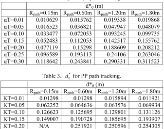
and sUGV as shown in Table 1-Table 3 given εe=0.05 m. Note that is represented by KT

for VP & PP and is represented by

UGV s

T

α for QC. From the tables, if we know α or K used in

the path tracking algorithm, the radius of the pathRpath, and the sampling period T, we can

determine the optimal look-ahead distance for the path tracking algorithm. If the path to

be tracked comprises of several circular curves with different radius, will be looked up

from the smallest

* 0 d

path 0

R because should be suitable for the worst case since the UGV has the most difficulty tracking the circular path with smallest radius.

* d

Table 1. * for VP path tracking.

0 d

d*0 (m)

Rpath=0.15m Rpath=0.60m Rpath=1.20m Rpath=1.80m

(54)

Table 2. * for QC path tracking.

0 d

d*0 (m)

αT=0.01 0.010629 0.015762 0.019338 0.019868 αT=0.05 0.016523 0.036821 0.047947 0.048079 αT=0.10 0.033477 0.072053 0.093245 0.099735 αT=0.15 0.052483 0.112053 0.142517 0.155762 αT=0.20 0.077119 0.15298 0.188609 0.208212 αT=0.25 0.096589 0.193113 0.24106 0.263046 αT=0.30 0.118642 0.243841 0.290331 0.311523

Table 3. * for PP path tracking.

0 d

d*0 (m)

KT=0.01 0.01298 0.01298 0.015894 0.011921

KT=0.05 0.062252 0.064636 0.063576 0.069934 KT=0.10 0.126623 0.125695 0.129801 0.131126 KT=0.15 0.149007 0.190728 0.185695 0.193907

KT=0.20 N/A 0.251921 0.250596 0.254305

KT=0.25 N/A 0.311391 0.313907 0.316689

KT=0.30 N/A 0.375762 0.379073 0.375894

B. Find dmax andβ for QC algorithm

According to QC algorithm, at different * 0

d R_path is calculated from quadratic curve

coefficient, A, as shown in Eqn. (1) where the relationship between A and Rpath can be

derived as A=1/(2R_path) when the UGV moves withRUGV =Rpath. Therefore, instead of looking

up * from

0

d R_path and αT, QC needs to look up dmax and β for each αT. We can find dmax

and β for each αT by using the information in Table 2 and nonlinear curve fitting based on

Eqn. (1). An example for finding dmax and β for one value of αT from each row of Table 2

On Network-based Control and Sensitivity Characterization of Mobile Robot in Intelligent Space

ABSTRACT

DEDICATION

To my parents, Phitaya and Sirima Vanijjirattikhan, and

my wife, Sukwida Manorangsan, for their endless love,

BIOGRAPHY

ACKNOWLEDGEMENTS

TABLE OF CONTENTS

LIST OF TABLES

LIST OF FIGURES

CHAPTER I

INTRODUCTION

CHAPTER II

ACCUMULATED EFFECT PARAMETER TUNING METHOD

FOR GEOMETRICAL PATH TRACKING OF WHEELED

MOBILE ROBOTS

ACCUMULATED EFFECT PARAMETER TUNING METHOD

FOR GEOMETRICAL PATH TRACKING OF WHEELED

MOBILE ROBOTS

(

)

[

]

(

)