KARP, STEPHANIE. Not in my Backyard: Suburban Forests and Climate Change. (Under the direction of Dr. Gary Blank).
Climate change will impact the suburban forest and the ecosystem services it provides.
Diversifying and increasing the amount of canopy cover are considered fundamental strategies
for mitigating impacts of climate change on the suburban forest. However, little is known about
communities most at-risk to adverse effects of climate change, especially in communities where
private homeowners manage trees. To understand which subdivisions are most at-risk, applied
historical ecology was used to provide a frame of reference for assessing the vulnerabilities of
suburban forests (n=76) throughout Fayetteville, North Carolina. Then I evaluated the
socio-economic characteristics and, using a Likert-scaled survey, the adaptive capacity of the
homeowners (n=76) within those subdivisions to mitigate and adapt the suburban forest. The
most at-risk subdivisions were evaluated for potential risk factors that could be more broadly
applicable for identifying at-risk subdivisions. The majority of trees in the study area had low to
moderately low vulnerability, with higher vulnerability species being at the southern or
eastern-most edge of their habitat range. Approximately half of the samples currently above 30%
canopy cover are predicted to fall below 30% due to the impacts of climate change on vulnerable
species. Evidence suggests that the modern-day presence of vulnerable species is related to (1)
subdivision age, (2) changes in the land cover that occurred during early settlement, and (3) land
use changes that occurred during the Great Depression and World War II. The strongest
evidence suggests that land abandonment and the rise of ruderal species following the Great
Depression is correlated with greater proportions of higher vulnerability species, indicating a
possible land use trend. The capability, willingness and knowledge of homeowners to mitigate
number of land use changes occurring between pre-European contact and today was found to
significantly improve the model for adaptive capacity from an adjusted R2 of 0.20, for income alone, to an adjusted R2 of 0.31. Within the sample, eight subdivisions were found to be at-risk to the adverse effects of climate change, none of which were high minority or low-income
communities. Two possible risk factors were found: (1) the number of land use changes that
occurred following the Great Depression and World War II and (2) the total number of land use
changes that occurred between pre-settlement and today; however, the results from Monte Carlo
simulations and Mantel-Haenzel testing were inconclusive. The results highlight the importance
of including the historical perspective to increase effectiveness of management by identifying
trends that may lead to greater risk, inform managers of possible outcomes for particular land
management practices, and help to guide or constrain management actions in the future.
Moreover, the historical perspective adds explanatory power to understanding of the current
suburban forest and its vulnerabilities, which can improve predictive models, thereby reducing
potential missteps. Additionally, the results are a cautionary tale against strictly relying on
socio-economics, as the most at-risk subdivisions were not highest minority or lowest income
communities. Nor should decision-makers neglect to consider future climatic conditions when
considering canopy cover improvement goals. Integrating historical, socio-economic, and
ecological factors into assessment, planning, decision-making, and management tools for
suburban forests is needed. While the complexity and dynamic nature of suburban landscapes
and tree vulnerability make identifying vulnerable subdivisions challenging, such understanding
is of vital importance for sustaining the ecosystem services that suburban forests can provide for
© Copyright 2018 by Stephanie Karp
by Stephanie Karp
A thesis submitted to the Graduate Faculty of North Carolina State University
in partial fulfillment of the requirements for the degree of
Master of Science
Natural Resources
Raleigh, North Carolina
2018
APPROVED BY:
_______________________________ _______________________________ Dr. Gary B. Blank Dr. George Hess
Committee Chair
ii
DEDICATION
I dedicate this thesis to my little research assistants, Abigail and Grant Karp, who offered
assistance in the field, many distractions, and more patience than can be asked of young children.
I also dedicate this to my husband, Oliver Karp, for encouraging me, even during the most
difficult times. I want to thank my aunt, Therese O’Toole, for her academic discussions,
guidance, and inspiration. I also want to thank my uncles, Jimmy O’Toole and Jim King, for
helping me at a crucial moment in my research. Lastly, I want to thank my father-in-law,
iii
BIOGRAPHY
My interests in people and the landscape began when I was a geography undergraduate in
2001 at the United States Military Academy at West Point, New York. After graduation, I was
commissioned as an officer in the United States Army and began training in human resource
management. After completing my training, I began a journey around the world, serving in a
variety of job positions. My diverse experiences lend to my understanding of the interface
between the human and natural environments. My interests include urban and suburban ecology,
land transitions, and conservation in the built environment. The coursework I have pursued has
sought to understand how various fields view the intersection of the suburban typology, the
iv
ACKNOWLEDGMENTS
I would like to thank my advisor, Dr. Gary Blank, who helped me to navigate my way
through this research. Thank you for letting me fall when I needed to fall, for keeping me from
trying to solve the world’s issues, and for helping to coalesce this paper.
I would like to thank Dr. Consuelo Arellano and Chandni Malhotra for their assistance
with the statistical analysis. I learned more about statistics and statistical analysis in our
discussions than a semester’s worth of statistics class. Chandni, you have a knack for explaining
v
TABLE OF CONTENTS
LIST OF TABLES ... vi
LIST OF FIGURES ... vii
Chapter 1: Introduction ... 1
Chapter 2: Methodology ... 11
Overall ... 11
Census Data ... 13
Survey ... 14
Historical Land Use and Land Cover ... 15
Tree Inventory and Rating ... 18
Chapter 3: Analysis ... 23
Chapter 4: Results ... 25
The Suburban Forest ... 25
Tree Species Vulnerability and Historical Land Factors ... 28
Adaptive Capacity and Socio-Economic Factors ... 37
At-Risk Subdivisions ... 41
Chapter 5: Discussion ... 46
The Suburban Forest ... 46
Tree Species Vulnerability and Historical Land Factors ... 49
Adaptive Capacity and Socio-Economic Factors ... 52
At-Risk Subdivisions ... 53
Chapter 6: Conclusion ... 55
References ... 59
APPENDICES ... 74
Appendix A: Suburban Forest Survey ... 75
Appendix B: Historical Land Use and Land Cover Procedures ... 79
T1: Pre-European Contact, pre-1730s ... 79
T2: Settlement, Natural Resource Exploitation, and War, 1730s - 1918 ... 82
T3: Fort Bragg and the Automobile, 1918 - 1939 ... 89
T4: WWII, 1939 - 1945 ... 95
T5: Post-WWII, 1945 - 2011 ... 99
Appendix C: R Code... 103
vi
LIST OF TABLES
Table 2.1 Tree Vulnerability Matrix ... 21
Table 4.1 Canopy Cover Summary Table ... 28
Table 4.2 At-Risk Subdivisions ... 42
Table 4.3 Comparing Socio-economic and Historical Land Factors by Sample,
Census Block, and At-Risk ... 45
vii
LIST OF FIGURES
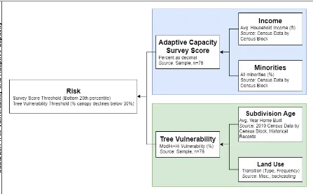
Figure 2.1 Suburban Tree Vulnerability and Adaptive Capacity Assessment Conceptual
Diagram ... 12
Figure 2.2 Determining the Number of Land Use Changes and the Types of Land Use Changes... 17
Figure 4.1 Histogram of the Percentage of Tree Species Vulnerable to Climate Change ... 26
Figure 4.2 Canopy Cover: Current, Expected Decline, and Expected Under Climatic Conditions... ... 27
Figure 4.3 Histograms of Historical Land Factors... ... 29
Figure 4.4 Forest Transitions of Fayetteville, North Carolina... ... 30
Figure 4.5 Pathways of Changes in Land Use Type... ... 32
Figure 4.6 Plots of The Percent of Vulnerable Tree Species and Historical Land Factors... ... 34
Figure 4.7 Spatial Relationship Between Tree Species Vulnerability and Historical Land Factors... ... 35
Figure 4.8 Modeling Tree Species Vulnerability and Historical Land Factors, QQ Plots... ... 36
Figure 4.9 Histograms for Adaptive Capacity Scores and Potential Socio-Economic Factors that may Influence Adaptive Capacity Scores ... 38
Figure 4.10 Spatial Relationship Between Adaptive Capacity Scores and Socio- Economic Factors.... ... 39
Figure 4.11 Scatterplots of Adaptive Capacity Scores and Log-Income, Proportion of Minorities, and Total Land Use Changes ... 40
Figure 4.12 Maps for At-Risk Subdivisions ... 43
Figure B.2 Fayetteville’s Transportation Network (Cohon, 1863) ... 83
Figure B.3 1782 Sketch of Cumberland County (top) and McDuffie’s Map of Cumberland County, 1884 (bottom) ... 84
viii Figure B.5 Current Longleaf Pine and Historical Railways and Roads, T2: Settlement and
Natural Resources Exploitation ... 89
Figure B.6 Photograph of the Rail Line extending to Fort Bragg, undated
(Tooker et. al, 2011) ... 91
Figure B.7 Changes in Urban Spread, 1923 to 1930.... ... 94
Figure B.8 Expanding Urbanization. Urbanization at the end of T2: settlement and natural resources exploitation period (Blue), T3: rise of the automobile (Purple),
T4: World War II (Green)... 96 Figure B.9 Current Land Use at the end of T5: Post-WWII.. ... 101
Figure B.10
1
CHAPTER 1 INTRODUCTION
Suburban forests provide many social, economic, and environmental benefits. In the
eastern part of the United States, for every dollar a city spends on street trees it will realize $3.25
(Raciti, 2006). Often the benefits trees provide go unnoticed until their decline begins to impact
these benefits. A perfect example of this is illustrated in the Baltimore-Washington,D.C. area
between 1973 and 1997. The canopy had declined approximately 15%, causing stormwater
runoff to increase by 19% at a cost of $1.08 billion, in addition to $24 million per year to remove
air pollutants (Cappiella et. al, 2005). This example also demonstrates the potential issues for
people living in the suburbs that could arise as a consequence of climate change. With nearly
half of the US population living in the suburbs and receiving ecosystem services the suburban
forest provides, understanding the vulnerabilities and adaptive capacity of suburban forests is
critical so that governments, subdivisions, and homeowners can plan for the future and act to
lessen the impact of climate change (Frey, 2012).
To understand how climate change my impact the suburban forest, both the caretakers of
the forest and the forest itself need to be considered (Dale, 1997). The research on suburban
forests, especially with respect to climate change, is relatively limited (Wilby and Perry, 2006).
The impacts that climate change will have on the suburban forest is just beginning to be
understood, with studies completed for several metropolitan suburbs to include Chicago, Illinois;
Atlanta, Georgia; Washington D.C., and Philadelphia, Pennsylvania (Brandt et. al, 2016; Lanza
and Stone, 2016; Brandt et. al, n.d.). However, these studies focus on only one form of the
2 not consider suburbs where privately managed trees dominate, suggesting that the definition of a
suburb is problematic.
In suburbs, where privately managed trees dominate the forest, the socio-economics of
the individuals within the suburb need to be understood to evaluate the management capabilities.
Much of the literature that evaluates the relationship between the suburban forest and its
caretakers has centered on the quantity of the forest, such as the amount of canopy (Heynen and
Lindsey, 2003; Danford et. al, 2014). However, little is understood about the relationship
between the quality of the suburban forest, especially with respect to climate change, and the
socio-economics of its caretakers.
While climate change will affect the current suburban forest in the future, a need to
understand relationships between historical legacies and current conditions exists. Past dynamics
not only form current conditions, but also inhibit future responses (Foster et. al, 2003). It is well
understood that historical land legacies influence both the ecosystem structure and function on
long temporal scales and may even be potentially irreversible (Christensen, 1989; Foster, 1992;
Goodale and Aber, 2001; Dupouey et. al, 2002; Foster et. al, 2003; Janowiak, 2017). This
knowledge of historical land legacies adds explanatory weight to our understanding of current
conditions of suburban forests. More importantly, such knowledge reduces missteps in planning
and managing the suburban forest for future climatic conditions (Foster et. al, 2003). More
importantly, historical legacies have been found to greatly improve climate feedback models
(Caspersen et. al, 2002). Despite the importance of including historical land legacies, no
research has focused on the relationship between historical land legacies and the presence of
3 policy makers and homeowners in planning for and enacting mitigative and adaptive strategies to
lessen impacts to the suburban forest (Dale, 1997).
Therefore, considering predicted climate change, I conducted an assessment of
vulnerability and adaptive capacity focused on a suburban forest. My research uses Fayetteville,
NC as a model for representing southeastern US suburban forests. Fayetteville is centrally
located in Cumberland County and is predominately suburban. Fayetteville has a wide range of
developments of various ages and socio-economic configurations. Additionally, Fayetteville has
well over a century of documented historical changes to the landscape. To assess the
vulnerability and adaptive capacity of suburban Fayetteville to predicted climatic conditions, I
used a dynamic framework outlined by Ramalho and Hobbs (2012). Their dynamic framework
evaluates the urban ecosystem on varied spatial-temporal scales, such as socio-economic land
use, urbanization age, past vegetative remnant configurations, and land use legacies. Ultimately,
this data will be used to evaluate where and who is at risk to ecosystem services degradation
given predicted climatic conditions (Allen et. al, 2010).
Many definitions of risk, vulnerability and adaptive capacity exist (Brooks, 2003). In
general, risk is a function of exposure and vulnerability (Cardona et. al, 2012; Brooks, 2003). To
further complicate the issue, there are two aspects of vulnerability: exposure and ability to cope
(Chambers, 1989). It is important to differentiate the social vulnerability from the biophysical
vulnerability, where adaptive capacity is a determinant of vulnerability (Brooks, 2003). As such,
risk is defined as a degradation of ecosystem services as a function of biophysical vulnerabilities
of tree species to climate change and the adaptive capacity of people living within a subdivision.
Biophysical vulnerability results from forest composition and structure. The average
4 respectively (Dwyer and Nowak, 2000). Theory suggests that species are more sensitive to
changes in the habitat when remaining habitats are below 30%, which was confirmed by
Banks-Leite et. al (2014), who found that both phylogenetic integrity and endemism declined when the
canopy cover was below 30%. Additionally, the results of empirical studies looking at habitat
changes and ecosystem function have suggested a threshold of 30 percent woodland cover
(Huggett, 2005). As such, the minimum threshold for tree vulnerability is 30 percent canopy
cover or if the canopy cover is already below 30% and declines.
The threshold for adaptive capacity using a Likert-scaled survey is the bottom 20th percentile or lowest quintile. Quintiles are commonly used by the US Census Bureau for
comparing income groups (Donovan, 2015). As such, adaptive capacity scores were grouped in
the same manner. Subdivisions that fall below both canopy cover and adaptive capacity score
thresholds are deemed at risk to ecosystem service degradation. This study assumes that the
absence of action to address ecosystems with vulnerable trees will result in ecosystem service
degradation given climate change (Murphy et. al, 2015). Thus, subdivisions with low mitigative
and adaptive capacity coupled with high numbers of vulnerable tree species are at the greatest
risk of ecosystem service degradation.
Tree vulnerability is defined as the degree of susceptibility of a tree species to climate
change and its ability to adapt to climate change (Glick et. al, 2011, Mach and Mastrandrea,
2014, Brandt et. al, 2016). I developed a tree species vulnerability matrix based on this
definition was created by using the suitability of the future habitat for a given tree species and its
ability to adapt. Similar matrices have been developed for forested habitats, but are based on
abundance data (Janowiak et. al, 2017; Iverson et. al, 2011). In urban areas, approximately
5 counterparts (Woodall, et. al 2010). Abundance data of forest tree species for urban and
suburban applications, therefore, may not be as relevant (Janowiak et. al, 2017). I used
ForeCASTS (Potter and Hargrove, 2013) to determine the suitability in lieu of the US Forest
Service (USFS) Climate Change Tree Atlas (Prasad et. al, 2007) because suburban trees can be
maintained in habitats that are outside of Importance Value Ranges used by the USFS. Within
the USFS Climate Change Tree Atlas, however, MODFACs provides readily available
information about the adaptability of tree species based on a multitude of factors to include life
history, disease, and pests (Matthews et. al, 2011). MODFACs was used in conjunction with
ForeCASTS to determine the vulnerability of a species. The species vulnerability was combined
with the adaptive capacity of suburban communities to determine the risk of ecosystem service
degradation.
To define the adaptive capacity of suburban communities, this study uses the
Intergovernmental Panel on Climate Change (IPCC) definition of adaptive capacity, which is
defined as “the potential or ability of a system, region, or community to adapt to the effects or
impacts of climate change” (McCarthy, 2011). Expanding on this, adaptive capacity is a
function of the willingness, knowledge, and abilities of communities to mitigate or adapt their
environment to climate change stimuli or their effects or impacts (Murphy et. al, 2015; Eakin and
Luers, 2006). Thus, subdivisions with low adaptive capacity are viewed as those that lack action
or capacity to employ adaptive or mitigative strategies (Murphy et. al, 2015). Adaptive and
mitigative strategies are complementary strategies to address climate change. Mitigation
strategies focus on the causes of climate change, while adaptation strategies center on
6 dependent. This study does not seek to determine the efficacies of any particular strategy nor to
determine the drivers of adaptive capacity, but rather uses common strategies as an indicator of
the mitigative and adaptive capacity (Smit and Wandel, 2006).
Adaptive capacity in this study was estimated using a survey based on common
mitigative and adaptive strategies presented by Brandt et. al (2016). The strategies from the
Brandt et. al (2016) study include resisting change, enhancing resiliency, and facilitating
transitions. These strategies include retaining biological legacies, maintaining and enhancing
native species, increasing biodiversity, and promoting diverse age structures. Strategies to
facilitate transitions include selecting tree species adapted to current and future site conditions,
introducing southerly species that are expected to adapt, and incorporating disease and
insect-resistant species (Brandt et. al, 2016). These strategies formed the basis for the questions used in
the survey.
The management and thereby, the capacity for adaptation, of the suburban forest is a
social endeavor (Wilby and Perry, 2006; Ordóñez and Duinker, 2014). Since, the suburban
forest has an inherent social component, adaptive capacity and the management of the suburban
forest is related to socio-economic factors. The quantity of canopy cover is commonly used to
predict the relationship between the management of the suburban forest and socio-economic
factors. Numerous quantitative canopy cover studies have found that higher levels of canopy
cover are correlated to higher income, neighborhood age, and inversely correlated to the
proportion of the total population made up by minority populations (Heynen and Lindsey, 2003;
Danford et. al, 2014). This study, however, seeks to understand the role socio-economics plays
in the managing the composition, particularly the vulnerability to climate change, rather than the
7 subdivisions, so two factors known to be related to the quantitative management of the suburban
forest, income level and minority populations, were explored as possible determinants of
adaptive capacity. While adaptive capacity seeks to understand the potential future implications
of managing and adapting the suburban forest, it is also important to understand the historical
factors that have led to the current composition.
There is a long debate among cultural geographers about how to look at the landscape, to
include the suburban landscape. Two schools of thought on how to look at the arrangement of
the landscape exist: as a chronological series of layers of landscape changes or as a temporal
process, whereby, a multitude of dynamic processes are occurring on varying temporal scales
(Crang, 1998; Heatherington et. al, 2017). The temporal process allows for one to view the
spatial dispersion of change, which was the approach taken in this study. The changes of interest
for this study are historical land use and land cover because of their impacts on forests
(Christensen, 1989; Foster, 1992; Goodale and Aber, 2001; Janowiak, 2017). Several methods
exist for determining historical land uses and land cover, some more quantitative and others
more qualitative. One promising quantitative approach is a back-cast approach, which has been
used in a few, relatively recent studies (Tayyebi et. al, 2015). The back-cast approach to
modeling land use and land cover changes is an alternative to forecasting. Back-casting begins
with defining desirable futures and working backwards to the current conditions. It is used to
identify pathways leading to desirable states. However, for historical land use and land cover
reconstruction applications, the direction is reversed. Reconstruction begins with defining the
oldest historical point and working forwards to current conditions. One recent study
reconstructed the historical land uses of the Ohio River Basin, where two reference land use
8 population censuses (Tayyebi et. al, 2015). However, this approach may lack the ability to
capture some of the more nuanced land use changes that can occur on a local level, depending on
the length of time under consideration, the accuracy and availability of historical data, and the
questions being asked (Christensen, 1989). A qualitative approach, alternatively, can capture
land use processes at a regional and local level that more generalized, quantitative approaches
cannot (Gragson and Bolstad, 2006). For this study a combined quantitative and qualitative
approach was used, where a historical narrative was generated for multiple critical time periods
and coupled with current land cover and land use datasets, previous research results, and
historical documents, such as census data, to reconstruct historical land uses and land covers.
Because land use and land cover are interrelated, these terms are often used
interchangeably (Anderson, 1976). Land use describes the human activities on the landscape,
along with the decisions about the use of land (Anderson, 1976; Nickerson et. al, 2015).
Meanwhile, land cover refers to the vegetative or manmade constructions on the surface of the
land (Anderson, 1976; Nickerson et. al, 2015). However, it is important to note that there is not
a singular land use or land cover classification system that is ideal and tends to be subjective
(Anderson, 1976). The USGS National Gap Analysis Program is a dataset of regionally distinct
vegetation based on the national vegetation classification level, suitable for use in reconstructing
land cover (GAP, 2011). There are three datasets applicable to the study area that classify land
use or are a hybrid classification of land use and land cover: Economic Research Service, Natural
Resources Conservation Service, and the US Geological Survey’s (USGS) National Land Cover
Database (NLCD). The Economic Research Service is a comprehensive land use dataset dating
back to 1945 (Nickerson et. al, 2015). While ideal for the topic of this research, the Economic
9 suitable for this study. The Natural Resources Conservation Service and the NLCD use a hybrid
classification system of both land use and land cover. The focus of the Natural Resources
Conservation Service database is agricultural, while the NLCD is focused on ecosystems,
biodiversity, climate change, and land management policies. The NLCD is based on the
Anderson Land Cover Classification System, which takes into special consideration the
definitions used by other agencies to categorize land uses, permits the use of vegetation as
surrogates for certain land use activities, and was designed for land use planning and
management activities (Anderson, 1976). Therefore, the NLCD is the best candidate for using to
reconstruct historical land uses in this study area. Differentiating between land use and land
cover is important in terms of modelling, where land cover is needed for physical environmental
models, while land use tends to be used for policy, planning, and management purposes
(Comber, 2008). Furthermore, the characteristics of land cover differ from land use in important
ways. Land cover classification the record of the vegetation on the surface of the earth tends to
be static, while land use is complex, where many simultaneous land uses can occur at any given
location (Comber, 2008). This study looks at both the physical and management aspects of the
suburban forest, hence the importance for differentiating land use and land cover.
There are three questions guiding my research. The first question looks at possible
historical factors that might result in higher portions of species of trees vulnerable to climate
change. Are there land use or land-cover legacy pathways or eras of development that are
correlated to the proportion of the number of species of trees vulnerable to climate change? The
second question seeks to understand the socio-economic factors that could limit a subdivision
from applying adaptive or mitigative strategies. Does income or the proportion of minorities
10 considered, different than subdivisions not at risk in the sample or from the subdivisions in the
study area?
Hypotheses:
1. There is a positive correlation between the percent of vulnerable tree species and
subdivision age, with mid-century subdivisions having the highest proportion of
vulnerable tree species.
2. There is a positive correlation between the percent of vulnerable tree species and
frequency of land use and land cover change.
3. There is a positive correlation between the percent of vulnerable tree species and land
use change and land cover pathways.
4. Adaptive capacity scores are positively correlated to income and negatively correlated
to the percent of minorities in a subdivision.
5. The mean of each factor for subdivisions identified as at-risk will be statistically
11
CHAPTER 2 METHODOLOGY Overall
In this study, I used Fayetteville, NC as a model for US southeastern suburban forests to
conduct a vulnerability and adaptive capacity assessment. First, I identified which tree species in
the southeastern suburban forest are vulnerable to climate change. Then, I determined the
subdivisions, categorized by historical land factors, where the greatest amounts of vulnerable tree
species occur. Next, I quantified the adaptive capacity of the different socio-economic
subdivisions. Lastly, I evaluated the subdivisions at risk of ecosystem services degradation.
Using the dynamic urban framework outlined by Ramalho and Hobbs (2012), a
multi-step process was used for this assessment (Figure 2.1). The initial multi-step was collecting, filtering,
and sorting already accessible data, which included average age of homes built, income and
demographics from Census data. Simultaneously, historical documentation was collected to
develop an historical narrative. The historical narrative was interpreted and, using a backcasting
method, the land use and land cover for 5 periods was determined. This was then analyzed to
determine the land use and land-cover legacy pathways, to include the frequency of change and
the types of changes for each subdivision. The next step was to sample suburban homeowners
and their lots throughout Fayetteville, NC to determine the mitigative and adaptive capacities of
homeowners and percentage of vulnerable tree species. A survey was used to assess the
mitigative and adaptive capacities at each sample site and at the same sample site, trees were
identified and quantified for each species. Later, both the survey and tree inventory were
tabulated, assigning each sample site a survey score and a percentage of vulnerable tree species.
12 and the selected socio-economic factors: incomes and percent of minorities. The percentage of
vulnerable tree species was analyzed to see if a correlation with subdivision age, land use, or
land-cover legacies existed. The last step was to determine subdivisions that are at risk of
ecosystem service degradation.
One important concept to consider is the characterization of the suburban forest. The
characterization of what makes an area suburban or not is difficult to discern as there are
numerous definitions available (Forsyth, 2012). Gianotti et. al (2016) presented a method that
qualitatively characterizes suburbs, making comparisons between different suburbs feasible.
Due to time constraints, this method was not used; however, this method may offer a solution for
comparing various suburban typologies in the future. As an alternative, Gordon and Shirokoff
(2014) characterize suburbs into three types: (1) exurbs or low density rural areas, (2) auto
suburbs, where dwellers commute via personal transportation, and (3) transit suburbs or
13 metropolitan suburbs that use advanced public transit systems (Gordon and Shirokoff, 2014).
The study area in this research is an auto suburb, which is different from the Chicago
metropolitan suburbs used in the Brandt et. al study (2016). Since the definition of a forest
differs from the collective of trees in the suburbs, the urban forest definition from Duinker et. al
(2015) was used, which defines the urban forest as including “[a]ny tree found within a city
boundary, whether planted or naturally occurring.” Trees were defined using the USFS Urban
Forest Inventory and Analysis definition: a woody perennial plant with a single well-defined
stem, definite crown, and a diameter of 3 inches (USDA Forest Service, 2016).
Census Data
US Census data for Cumberland County was used to determine subdivision age, the
percentage of minorities (US Census Bureau, 2010a), and income (US Census Bureau, 2010b)
for each census block. Census blocks are statistical areas that are bounded by a variety of
visible features, such as streets, streams, and select property lines (US Department of Commerce,
1994). Census blocks are the smallest statistical areas with accessible social-economic data and
was found to be generally consistent with politically and socially recognized subdivisions (City
of Fayetteville, 2017a). Subsequently, the census block was used as a proxy for subdivisions.
Overall, 118 census blocks make up the study area.
The City of Fayetteville has overlapping relationships and responsibilities with outlying
communities, including Fort Bragg, Hope Mills and Spring Lake (City of Fayetteville, 2017b).
Since these outlying communities are still socially, culturally, and, in some regards, politically
unique from Fayetteville, they were not included as part of the study area.
In the census report, the age of the census block is equivalent to the year when the
14 determine home ages prior to 1950. Using the historical maps collected for the historical land
use and land-cover, the census blocks recorded as 1950 in the dataset were re-evaluated to
determine what decade the majority of the census block was built; either 1950 or earlier. Census
blocks were not dated to earlier than 1900, as only two census blocks cover the area of settlement
that occurred between the 1730s and 1900. No census blocks were recorded with dates between
1930 and 1950 for several reasons. First, this period starts with the Depression and was followed
by World War II, a period of limited residential development. Furthermore, of the few homes
that were built during this period, many of them were built on land cleared for development in
the 1920s, thus filling in subdivisions. Lastly, the criterion is based on the majority of homes in
a census block. While homes were built during this period, they did not constitute the majority
of a census block.
Survey
The suburban forest survey asks 26 questions to determine the awareness, willingness,
and ability of an individual to use these mitigation and adaption strategies (see Appendix A).
This survey was approved by North Carolina State University’s Institutional Review Board for
the Protection of Human Subjects in Research (Protocol # 11714). Several questions pertain to
financial and physical capabilities that some participants chose not to answer. Non-responses
were not included in the overall score. The Likert scale was used, where parametric testing can
be used (Sullivan and Artino Jr., 2013). Using the Likert scale, each response was assigned a
point value, with higher values assigned to responses that support a mitigative or adaptive
strategy. The mean of the responses was the individual’s mitigative and adaptive capacity score.
Subdivisions with large proportions of tree species vulnerable to climate change and low
15
Historical Land Use and Land Cover
The method used for part of this research was a combination of both quantitative and
qualitative approaches. First, a historical narrative was generated for five critical time periods.
This narrative was then quantitatively interpreted using research, historical maps, records, and
census data. Finally, the current land use/land cover quantitative datasets and the quantitative
interpretations were back-casted to estimate the historical land use and historical land cover for
each time period for each census block. From this data, the frequency of changes and the types
of changes and pathways for land use and land cover was determined. To capture possible
gardening trends that may have influenced the composition of suburban forests, particularly the
presence of vulnerable tree species, the age of the subdivision was determined using census data
and historical maps.
The temporal frame for constructing the historical land use and land cover begins prior to
European contact and ends in 2017. The temporal frame is divided into five periods. Each
period remains relatively constant in terms of development during a given period. The periods
are demarcated by significant events, such as a new technology or war, that result in dramatic
changes in the landscape. These periods include: pre-European contact to 1730s (T1), with an
influx of European settlers; 1730s to 1918 (T2), marked by the new railroad line,
industrialization, and natural resource exploitation; 1918 to 1939 (T3), when Fort Bragg was
permanently established and the automobile became commonplace; 1939 to 1945 (T4), when
incoming troops and returning troops begin to settle in Fayetteville; and the post-war period,
from 1945 to 2017 (T5), with the conception and continuation of suburbia.
The decennial census reports from 1880 to 2010 for Cumberland County from the
16 land and woodlands (Manson et. al, 2017). The census block age, as discussed earlier, was also
used to evaluate when land became urbanized. The census data, coupled with historical research
reports, historical maps, and modern research, especially longleaf pine research, were used to
develop a historical narrative. The historical narrative was used to interpret the land use and land
cover for each period. The interpretation provided quantitative guidelines for calculating the
land use and land cover for each period. The current or baseline maps were used to develop the
land use and land cover for the first period, pre-European contact (T1), which has the fewest land
use and land cover categories, primarily due to the lack of more detailed data. The second
period, T2: settlement and natural resources exploitation, was based off the first map, where
elements were added or removed in accordance with the interpretation of the historical map.
However, the changes for the period of settlement and natural resources exploitation period (T2)
were checked to ensure that they made sense with the baseline map. Subsequent periods were
17
Figure 2.2 Determining the Number of Land Use Changes and the Types of Land Use Changes. After each period is estimated, the number of changes is recorded based on the amount of acres to a category. For example, between the settlement and natural resources exploitation period (T2) and the T3: rise of the automobile period, the land transitioned from
18 I generated a baseline map for the land cover using data from the USGS National Gap
Analysis Program (GAP) from 2011. The baseline land cover map displays the macro group
national vegetation classification level, which features regionally distinct vegetation (GAP,
2011). The baseline map for the land use was generated using data from the USGS National
Land Cover Database (NLCD) from 2011. Both maps are raster, but slight variations in cell size
exist, so caution should be exercised when selecting baseline maps. While the baseline maps
offer relatively accurate resolution to approximately 1 acre (GAP, 2011), it is important to note
that resulting representational historical data derived from these baseline maps are not intended
to provide the same resolution. Rather, this data provides a coarse resolution, approximating the
land-cover and land use based on available research and historical maps. It is assumed that this
coarse resolution should hold true down to the census block level, where the average census
block is 473.6 acres and the smallest census block is approximately 101 acres. Additionally, it is
important to evaluate the applicability of this method to other cases. The Census Bureau’s
criteria for a census block establishes a minimum of 30,000 square feet, which is approximately
0.69 acres (US Department of Commerce, 1994). While not applicable to this case, the method
employed may not be applicable to regions where census block areas do not correlate with
representational historical maps or historical data. See Appendix B for procedures for historical
land use and land cover reconstruction.
Tree Inventory and Rating
Tree data was collected based on standard sampling and inventory protocols used by
i-Tree (Nowak et. al, 2008). Samples were determined using a randomized grid (Blood et. al,
2016). An 18 x 15 square (470 acres/square) grid was applied to the study area using fishnet in
19 each grid cell. The nearest residential intersection to this point was selected as a sample site.
Any grid cells that did not have a point inside of the study area was not included. Additionally, 6
grid cells with a point inside the study area lacked any residential intersections and were
excluded. Mobile home parks were excluded as they are land renters, while mobile homes on
land owned by the same person were included in the study. Condominiums and townhouses
were included, as well. Lastly, the absence of trees did not preclude a homeowner from
participating. The total number of potential sample sites was 119, from which 76 samples were
obtained. Maps produced in ArcGIS, however, show 61 census blocks, as some census blocks
had multiple samples and were averaged.
A similar sampling method employed by Nitoslawki and Duinker (2016) to evaluate tree
diversity in suburban developments was used. Starting clockwise at the nearest intersection,
homeowners were asked to participate in the study. Homeowners must have been above the age
of 18. If the homeowner did not wish to participate, the homeowner to the left of the original
randomly selected home was asked, and so on until a homeowner chose to participate in the
study. When a homeowner opted to participate, they were provided a written survey (Appendix
A) to complete and all trees on the property were identified, quantified, and recorded.
In the field, a variety of field guides were used to verify tree species. The main resource
was Katherine Kirkman’s Native Trees of the Southeast (2007). Trees that were unfamiliar and
not identifiable in field guides were photographed and subsequently researched. Most of the
photographed trees were exotic species that are available in local nurseries. Tree species were
recorded and counted for each property. Trees were then evaluated using the tree vulnerability
20 The tree vulnerability matrix evaluates both the habitat suitability and the adaptability of
a species based on a multitude of factors to include life history, disease, and pests. The habitat
suitability model used was ForeCASTs. From ForeCASTS, the “Present and Future Ranges”
maps were used for the matrix and are based on the Hadley climate model, lower emissions
scenario (B1) to the year 2050 (Potter and Hargrove, 2013). On these maps, green represents
new habitat in 2050, red represents areas that are currently suitable, but expected to be unsuitable
in the future, yellow represents areas that are both currently and projected to be suitable in the
future, and white represents areas beyond the habitat range. It is important to note that all
species distribution models, such as the USFS Climate Change Tree Atlas and ForeCASTS, have
limitations. These limitations include grid cell size, number of cells needed, and assumptions
about biotic interactions, to include human interactions (Iverson and Hargrove, 2014). In
ForeCASTS, a grid cell is 4 square kilometers and the study area is approximately, 230 square
kilometers or approximately 57 grid cells. To overcome uncertainties associated with the limited
number of grid cells for the study area, a regional approach, which is more robust, was used
(Littell et. al, 2011). Because more than one category of suitability can be found within a region,
the tree vulnerability matrix categorizes the suitability based on both the dominant category on
the ForeCASTs map and the second most dominant category. (First color is the dominant color,
2nd is minor compared to dominant). Green represents future suitability. Green-Yellow
represents future suitability, although limited areas might be suitable now and in future.
Yellow-Green represents both current and future suitability, but some areas might only be suitable in the
future. Yellow represents both current and future suitability. Yellow-red represents both current
and future suitability, but some areas might be unsuitable in the future. Red-Yellow represents
21 represents habitats expected to be unsuitable in the future. White represents areas not currently
or predicted to be suitable in the future. Because the habitat suitability model does not take into
account biological and disturbance factors, MODFACs was used to evaluate adaptability of
species. MODFACs is a score system based on current literature that evaluates 9 biological and
12 disturbance factors. These factors can modify the interpretations of the future habitat
suitability model. For example, if the future habitat of a species currently present is predicted to
be unsuitable, then extirpation is likely. However, if the species is highly adaptable, then the
species could do better than the habitat suitability model suggests. Species with a MODFACs of
greater than 0 (+), are more adaptable and may do better than modelled, while species with a
MODFACs score of less than 0 (-) are less adaptable and may do worse than modelled (Table
2.1).
Table 2.1 Tree Vulnerability Matrix
MODFACS
Decreasing in Species Adaptability
VHi+ Hi+ Lo+ Minimal Lo- Hi- VHi-
F or eC A S T S Dec re as in g in H ab it at Su it ab ili ty
Green Low Low Low Low Low Low Low
Green-Yellow Low Low Low Low Low Low Low
Yellow-Green Low Low Low Low Low Low Low
Yellow Low Low Low Low Low Low Low
Yellow-Red ModLo ModLo ModLo Mod Mod Mod Mod
Red-Yellow Mod Mod Mod ModHi ModHi ModHi High
Red ModHi ModHi ModHi High High High High
White ModHi ModHi ModHi High High High High
22 For species not identified in the ForeCASTS model or MODFACs database, a literature
review was conducted. Pests, pathogens, climate-related disturbances, and hardiness zones were
used as proxies for both habitat suitability and adaptability (Hunter, 2011). Species similar to
forest species used in ForeCASTS and MODFACs, were categorized the same, unless the
literature review suggested a higher or lower categorization. Species were categorized using the
same categories as the tree vulnerability matrix: low, moderately low, moderate, moderately
high, and high vulnerability.
The total species for each sample were tabulated, indicating the species richness for each
sample. Using the tree vulnerability matrix, species categorized with high and moderately high
vulnerability were summed together to determine the total species vulnerable. The proportion of
tree species vulnerable equals the sum of species categorized with high and moderately high
vulnerability in the sample divided by the total species in the sample. For example, a site has
four species, one of which is categorized as high vulnerability and two categorized as moderately
high vulnerability. The total vulnerable species is three and the proportion of species vulnerable
to climate change is three divided by four total species or 75%. Subdivisions with higher
proportions of tree species vulnerable to climate change along with low adaptive capacity scores
23
CHAPTER 3 ANALYSIS
SAS® software v 9.4.1 (SAS Institute Inc., 2016) was used for all analyses. The
procedures used for the descriptive statistics for all variables were MEANS, CORR, REG,
UNIVARIATE, FREQ, and SGPLOT. Income was transformed using a log transformation to
use for linear regression analysis. The percent of tree species vulnerable to climate change was
transformed using a square root transformation to address the skewness and for regression
analysis.
Socio-economic factors that could inhibit a subdivision from applying adaptive or
mitigative strategies were evaluated using Pearson’s correlation. A linear regression model was
fit for adaptive capacity scores, the dependent variable, to further explore the relationship. Low
adaptive capacity was defined as the lower 20th percentile of adaptive capacity scores and was
calculated using R version 3.4.3 software (R Core Team, 2017). See Appendix C for code.
Possible historical factors (land use legacies, land-cover legacies, and development ages)
that might result in higher portions of tree species vulnerable to climate change were explored.
Pearson’s correlation and partial correlation were used to assess the relationship between the
percent of tree species vulnerable to climate change and historical factors. A multiple linear
regression analysis was conducted between historical land factors and the percent of vulnerable
species.
The National Land Cover Database 2011 USFS Tree Canopy (Cartographic) was used for
determining the current canopy cover of each census block (Homer et. al, 2015). To estimate the
proportion of the canopy cover that is vulnerable, species richness was used as a proxy (Conway
24 proportion of species vulnerable to climate change found from the sample within that census
block (Eqn 1). For example, a sample in a census block with 50% total canopy cover, four total
species inventoried, and one species vulnerable to climate change, the proportion of the total
canopy cover that is vulnerable is 12.5%. When calculating the canopy cover under future
climatic conditions, the worst-case scenario was used: extirpation of all vulnerable species. The
canopy cover under future climatic conditions is the current canopy cover less the proportion of
the canopy that is vulnerable (Eqn 1). Using the previous example, the predicted canopy cover
would be 37.5%.
𝐶𝑎𝑛𝑜𝑝𝑦 𝐶𝑜𝑣𝑒𝑟𝑓𝑢𝑡𝑢𝑟𝑒= 𝐶𝑎𝑛𝑜𝑝𝑦 𝐶𝑜𝑣𝑒𝑟𝑐𝑢𝑟𝑟𝑒𝑛𝑡− (𝑉𝑢𝑙𝑛𝑒𝑟𝑎𝑏𝑙𝑒 𝑆𝑝𝑒𝑐𝑖𝑒𝑠 𝑅𝑎𝑡𝑖𝑜 ∗ 𝐶𝑎𝑛𝑜𝑝𝑦 𝐶𝑜𝑣𝑒𝑟𝑐𝑢𝑟𝑟𝑒𝑛𝑡) (𝐄𝐪𝐧 𝟏)
If the future canopy is predicted to decrease below 30% or if the current canopy cover is
already below 30% and is predicted to decline further, then the census block was deemed to be at
risk of ecosystem service degradation.
Subdivisions at risk of ecosystem degradation due to the impact of climate change on
trees was defined by having low adaptive capacity scores (20th percentile and below) and
canopies predicted to decrease below 30% or if currently below 30%, then any further decline.
Socio-economic and historical land factors showing a possible relationship with at-risk
subdivisions were tested for association using a Monte Carlo randomized Exact Fisher Test and
25
CHAPTER 4 RESULTS
Between February and March 2018, I worked with a statistical consulting team. Dr.
Consuelo Arellano and graduate student, Chandni Malhotra were responsible for all the
statistical analyses that were conducted for this study. Everything in this section, with the
exception of all the figures and the land use and land cover pathway results, are from the
statistical consulting report prepared by Dr. Arellano and Chandni Malhotra (Arellano and
Malhotra, 2018).
The Suburban Forest
The tree tree inventory occurred at 76 random plots, corresponding with homeowners
who respondeded to the adaptive capacity survey. The plots varied in size, depending on the
homeowner’s lot size. Plots were varied in subdivision age, dating from 1914 to 2010. The
suburban forest of Fayetteville, NC can be broadly characterized as a temperate forest with a mix
of hardwood and softwood tree species. Oak-pine is the dominant forest type, accounting for
44% (416) of the total trees inventoried (947). The remaining forest is a hodge-podge of species,
most of which are common in the local nurseries. Overall, the 947 trees are comprised of sixty
different species. Of the total number of trees, three species made up approximately 50% (475)
of the trees: Flowering Dogwood, Longleaf Pine, and Loblolly Pine, in descending order.
Twenty-two percent of the trees were the Flowering Dogwood, a popular native ornamental tree.
Two species identified in the study area are characterized as invasive: Callery Pear and Mimosa
(EDDMapS, 2018). The average number of trees per sample site was 12 trees. Two sample
26 Sixty (6.3%) of the trees were categorized as having a moderately-high vulnerability to climate
change and none were categorized as high vulnerability.
The percent of tree species categorized as moderately high and high vulnerability to
climate change within each sample (n = 76), ranged from 0% to 100% with a mean of 18.42%.
The average number of species per sample site is 4 species. There were 60 species identified in
the study area, of which 30% (18) were categorized with moderately high vulnerability to
climate change (Appendix D). None were categorized with high vulnerability to climate change.
Eight of the 18 vulnerable species (44%) are at the southern or eastern edge of their habitat
ranges. Just under half (42%) of the samples had no species vulnerable to climate change,
causing the distribution to be heavily skewed (Figure 4.1).
Tree species richness vulnerability was used as a proxy for canopy cover vulnerability
(Conway and Bourne, 2013). Canopy cover under future climatic conditions is the current
canopy cover less the species richness vulnerability (Eqn 1). Spatially, there is a small cluster of
subdivisions exhibiting canopy risk that is located approximately five miles west of the historic
city center. These subdivisions vary in the proportion of vulnerable species and the current
27 amount of canopy cover (Figure 4.2). The current canopy cover for the study area covers
approximately 21,140 acres out of approximately 55,885 acres.
A total of 25 samples (33% of observations) had canopy covers that were expected to
decline below 30% or are currently below 30% and are expected to decline due to climate change
(table 4.1). Of the 18 samples currently below 30% canopy cover, 39% (7) were not expected to
decline further due to climate change. Approximately, one quarter of the subdivisions with
canopy covers above 30% were expected to decline below the threshold. More than half of the
Figure 4.2 Canopy Cover: Current, Expected Decline, and Expected Under Climatic Conditions. Figure (a) shows the proportion of species vulnerable to climate change (n=76). Figure (b) shows the current canopy cover. Figure (c) illustrates the canopy cover under climatic conditions, where the current canopy declines by the percent of vulnerable species. There appears to be a cluster of subdivisions exhibiting canopy risk, located approximately five miles west of the historic city center.
Historic City Center
Historic City Center
28 subdivisions with canopies expected to decline below the 30% threshold were subdivisions that
are currently above the threshold.
Tree Species Vulnerability and Historical Land Factors
Several historical factors might result in higher proportions of tree species vulnerable to
climate change. Subdivision age, the frequencies of land use and land cover changes, and the
types of land use and land cover changes were analyzed to see if they are factors that indicate
high proportions of tree species vulnerable to climate change. Land use and land cover changes
were reported over five periods. The year subdivisions were built ranged from 1914 to 2010.
Approximately 50% of the samples date from 1978 or later (Figure 4.3). Both the frequency of
land use changes and land cover changes between each of the five periods is reported in discrete
values. The average total number of land use changes per subdivision is five (n=76), while the
Table 4.1 Canopy Cover Summary Table
Current Canopy Cover Canopy Cover Excluding Vulnerable Species Total Risk
> 30% Decrease, but remain > 30% 19 No
> 30% < 30% 14 Yes
> 30% No Change 25 No
< 30% Decrease 11 Yes
< 30% No Change 7 No
29 most frequent number of land cover changes is eight. In general, the values have a relatively
small range and tendency for observations to concentrate around one or two values (Figure 4.3).
Historical studies of forests have found that forest changes occur in predictable ways. In
general, a large decline in forest cover occurs when societies undergo economic development and
industrialization. After that, the trend reverses and forest cover increases slowly. This occurs
simultaneously with increasing urbanization (Mather, 1990; Walker, 1993; Mather and Needle,
1998; Rudel, 1998; Rudel et. al, 2005). However, this overall trend occurs on various scales, may
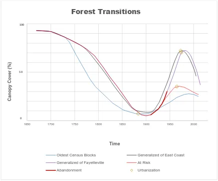
30 vary from one place to another, and is not inevitable (Rudel et. al, 2005). In this study, this general
trend of canopy decline followed by a slow increase in canopy corresponds with the land use and
land cover changes across the entire study area. This study also produces evidence that land use
and land cover changes varied among subdivisions. Subdivisions closer to the historical town
center underwent this trend earlier than other subdivisions (as indicated in the blue line in Figure
4.4). While at-risk subdivisions followed the same general trend, it was when these subdivisions
transitioned to urbanization that is notable.
Figure 4.4 Forest Transitions of Fayetteville, North Carolina. Fayetteville, like the forests on the eastern coast of the United States follows a general trend of deforestation, followed by a slow increase in canopy until multiple land use pressures begin to change the canopy again (Drummond and Loveland, 2010; Houghton and Hackler, 2000). Fayetteville, however, reaches its minimum earlier and reaches its maximum later. Early in the 20th century, a trend of abandonment of farm land and field succession persisted (Manson et. al, 2017). This trend had not fully reversed until after 1940. At-risk subdivisions begin heavy urbanization directly following this period. Final canopy cover estimates were from Nowak and Greenfield, 2010.
1650 1700 1750 1800 1850 1900 1950 2000
C a n o p y C o v e r (% ) Time
Forest Transitions
Oldest Census Blocks Generalized of East Coast
Generalized of Fayetteville At Risk
Abandonment Urbanization
100
50
31 The most common pathway of land use changes follows the general downward trend of
canopy cover resulting from industrialization, intensive natural resource exploitation, railroads,
and movement towards agricultural land uses. However, the pathway departs from the expected
trend of a slow increase in canopy cover between T3: rise of the automobile and T4, following the
Great Depression and the onset of World War II. This departure from the general canopy cover
trend in the eastern United States and Fayetteville, in general, is due to the abandonment of
agricultural lands, leading to a rise in ruderal species (Manson et. al, 2017). Any gains in canopy
cover were minimal before urbanization occurred. This particular pathway of land use changes,
FP_P_JO_ABC, accounts for 36% of the land use change pathways that occurred in the study area.
Nearly half of the subdivisions with this pathway showed canopy risk. Six of the eight (75%)
32
Figure 4.5 Pathways of Changes in Land Use Type. Approximately 1/3 of the samples had the same land use change pathway, FP_P_JO_ABC. Seventy-five percent of risk samples were from this same pathway. The remaining at-risk samples followed similar pathways: FP_N_JO_ABC and
33 Forty-seven unique land cover change pathways occurred between pre-European contact
(T1) and the post-war period (T5). The most common land cover change pathway (70% of
pathways) mirrors the most common pathway for land use changes, where a rise in ruderal
species occurs between T3: the rise of automobile and T4: World War II due to field
abandonment. Of the 53 samples that followed this general land cover pattern to the beginning
of T4: World War II, over 70% were converted to suburbs. Those samples that converted to
suburbs following the rise of ruderal species between T3: the rise of the automobile and T4:
World War II account for 76% of the subdivisions with canopy risk and 88% of the at-risk
subdivisions.
Subdivision age, the frequency of land use changes, and the frequency of land cover
changes were explored to see if they are factors that might result in the presence of tree species
vulnerable to climate change. Both the scatterplots and spatial mapping of the percent of tree
species vulnerable to climate change and historical factors do not appear to show any strong
34
35 Pearson’s correlation coefficient was used to test for relationships between the percent of
trees vulnerable to climate change and historical land factors. Only three historical land factors
had a correlation with the percent of tree species vulnerable to climate change: the number of
land cover changes between T2: settlement and natural resources exploitation and T3: rise of the
automobile, the number of land use changes occurring between T3: the rise of the automobile
and World War II (T4), and subdivision age. However, all are weak, non-significant,
36 Three models were fitted for the percent of tree species vulnerable to climate change.
The models were fitted with (1) the number of land use changes between T3: the rise of the
automobile and T4: World War II, (2) the number of land use changes between T3: the rise of
the automobile and T4: World War II and subdivision age, and (3) the number of land use
changes between T3: the rise of the automobile and T4: World War II and the number of land
cover changes between the period of settlement and natural resource exploitation (T2) and T3:
rise of the automobile (adj. R2 = 0.01, 0.02, 0.03, respectively). None of the models explained more than 3.5% of the variation and therefore no meaningful linear relationship exists between
the three identified explanatory variables and the percent of tree species vulnerable to climate
change. The same weak relationships were found when a randomization test for model F was
run (Cassell, 2002). It is likely that the weakness of the model might be explained by the high
number of samples characterized by an absence of trees species vulnerable to climate change
(42%), shown as the row of horizontal sample points (Figure 4.8). A relationship with historical
land factors does appear to exist with the samples where vulnerable tree species are found.
While there is no strong evidence about whether the percent of vulnerable tree species can be
Model 1 Model 2 Model 3
37 explained by historical land factors, indicators do suggest a possible relationship and point to
possible future studies.
Adaptive Capacity and Socio-Economic Factors
The survey included 76 random respondents from a wide range of socio-economic
backgrounds across the study area. Adaptive capacity scores (n = 76), on a 0 to 1 scale, range
from 0.54 to 0.92. Adaptive capacity scores show a symmetrical distribution with a mean of
0.71, 95% CI [0.69, 0.73], indicating that the sample size is adequate. Two factors contributing
to adaptive capacity scores were assessed: income and proportion of minorities. The mean
income of the 76 samples is $51,432.30, after a log10 transformation (M = 4.67, 95% CI [4.62,
4.71]). The mean for the proportion of minorities is 52.76%, 95% CI [46.92, 55.59] (Figure 4.9).
Both income and the proportion of minorities appear to cover a sufficient cross-representation of
38
39 Income and the proportion of minorities were explored to see if they were factors that
could inhibit subdivisions from applying adaptive or mitigative strategies to overcome the
impacts of climate change on the suburban forest. The spatial mapping of adaptive capacity
scores and socio-economic factors suggest possible relationships (Figure 4.10).
Moreover, scatterplots of adaptive capacity scores and socio-economic factors also support the
possibility of relationships (Figure 4.11). While not originally considered a factor, the scatterplot
of the total land use changes variable and adaptive capacity scores showed an overall negative
40 linear trend, indicating that this relationship should be considered (Figure 4.11). It is important
to note that the observation of 8 total land use changes might be the cause of this negative trend.
Using Pearson’s Correlation Coefficient, adaptive capacity scores were found to be
moderately correlated with log-income (r = 0.46, p < 0.0001). Both the total land use changes
variable and the percent of minorities were found to have a weak, negative correlation with
adaptive capacity score (r = -0.20, p = 0.08; r = -0.25, p = 0.03; respectively). The correlation
41 with total land use changes variable significantly improves after controlling for logincome (r =
-0.3851; p = 0.0006), which supports the importance of these two variables when modeling
adaptive capacity scores.
The models fitted for adaptive capacity scores were (1) log-income, (2) total land use
change variable, and (3) both log-income and the total land use change variable (adj. R2 = 0.20,
0.03, and 0.31, respectively). In model 3, income is a more important factor for determining
adaptive capacity scores than total land use change variable (StdB = -0.36, 0.56, respectively).
In the absence of adaptive capacity scores, the total number of land use changes and median
household income can be used to estimate adaptive capacity scores using:
𝐴𝐶𝑆̂ = −0.278 + (−0.038) ∗ 𝐿𝑎𝑛𝑑 𝑈𝑠𝑒 𝐶ℎ𝑎𝑛𝑔𝑒𝑠𝑇𝑜𝑡𝑎𝑙+ 0.255 ∗ 𝐿𝑜𝑔10𝐼𝑛𝑐𝑜𝑚𝑒 (𝐄𝐪𝐧 𝟐)
At-Risk Subdivisions
Subdivisions at-risk were defined as having adaptive capacity scores that fall below the
20th percentile and canopy covers that decrease below 30% or any decline if the canopy cover is currently below 30%. The 20th percentile adaptive capacity score is 0.62. Sixteen of 76 (21.1%) homeowners surveyed had adaptive capacity scores below the 20th percentile threshold.
Twenty-five of 76 (32.9%) samples had canopies that were at risk of decreasing below the 30% canopy
threshold or were already below 30% and are at risk of further decline in ecosystem services.
Overall, eight out of 76 samples (10.5%) had adaptive capacity scores below the 20th percentile and large proportions of vulnerable tree species that may result in a decline in canopy below the