Rank-Based Statistical Methodologies for Quantitative Trait Locus Mapping
Fei Zou,*
,1Brian S. Yandell
†and Jason P. Fine
†*Department of Biostatistics, University of North Carolina, Chapel Hill, North Carolina 27599 and †Department of Statistics, University of Wisconsin, Madison, Wisconsin 53706
Manuscript received April 13, 2003 Accepted for publication July 25, 2003
ABSTRACT
This article addresses the identification of genetic loci (QTL and elsewhere) that influence nonnormal quantitative traits with focus on experimental crosses. QTL mapping is typically based on the assumption that the traits follow normal distributions, which may not be true in practice. Model-free tests have been proposed. However, nonparametric estimation of genetic effects has not been studied. We propose an estimation procedure based on the linear rank test statistics. The properties of the new procedure are compared with those of traditional likelihood-based interval mapping and regression interval mapping via simulations and a real data example. The results indicate that the nonparametric method is a competitive alternative to the existing parametric methodologies.
Q
UANTITATIVE genetics has developed rapidly, methods.KruglyakandLander(1995) apply the lin-ear rank statistics to interval mapping, which is imple-especially with progress in DNA-based geneticlinkage maps. Various statistical approaches have been mented in the latest version of Mapmaker/QTL ( Lin-colnet al.1993) and Qlink (Drinkwater1997). However, proposed to identify QTL by using molecular markers,
such asSax’s (1923) single-marker t-test,Landerand the method tests only for the presence of a QTL and does not provide an estimate of the phenotypic effect
Botstein’s (1989) maximum-likelihood-based interval
mapping,HaleyandKnott’s (1992) regression inter- of the QTL. In this article, we extend the rank-based test statistic to the estimation of the quantitative trait val mapping, andZeng’s (1993, 1994) andJansenand
effects.
Stam’s (1994) composite interval mapping.
Rank-based methods play an important role in non-All the methods mentioned above are based on the
parametric statistics. The linear rank statistic has been normality assumption (or other parametric models) for
widely used in practice and its theoretical properties the component distributions. The normal mixture
have been thoroughly studied (HajekandSidak1967; model is the default analysis and is implemented in the
Hajek 1968). For linear regression, estimates of the
widely used packages Mapmaker/QTL (Lincoln et al.
regression coefficients based on linear rank statistics are 1993) and QTL Cartographer (Basten et al. 1997).
available and have efficiency and robustness properties Many traits, however, are not normally distributed. An
that are similar to those of the linear rank statistics. example is tumor counts, which arise in cancer studies
In this article, we adapt the existing methodology to and often appear to follow a negative binomial (
Drink-construct rank-based estimates for genetic effects under
waterand Klotz 1981). Naively assuming normality
the assumption that the underlying QTL component of the underlying distributions greatly simplifies the
distributions have the same form and differ only by a form of the likelihood function. A problem is that if
shift. This appears to be the first attempt to apply linear this assumption is violated, then false detection of a
rank-based estimates directly to the interval mapping major locus may occur (Morton1984).
and thus complements existing parametric methods. When the underlying distributions are suspected to
Simulations are conducted to compare the relative effi-be nonnormal, one strategy is to use a likelihood
ap-ciencies of the nonparametric and parametric methods proach after transforming the data using, for example,
under a variety of distributions. the Box-Cox transformation (DraperandSmith1998).
The article is arranged as follows. In the next section, However, an appropriate transformation may not exist
we briefly introduce linear rank statistics and related or may be difficult to find. Also this approach can raise
estimation procedures for regression analysis. In
non-serious issues of interpretation and the transformation
parametric interval mapping, the estimates of QTL
involves an extra parametric assumption.
effects are proposed in the context of interval mapping. An alternative approach is to consider nonparametric
In numerical studies, the relative efficiencies of the
proposed estimates are compared with the parametric estimates in simulation studies and the methods are
1Corresponding author: Department of Biostatistics, University of
illustrated in backcross data where the phenotype has
North Carolina, 3107D McGavran-Greenberg Hall, CB 7420, Chapel
Hill, NC 27599. E-mail: [email protected] a highly skewed distribution. Inconclusion and
y|Xi)⫽F(y⫺Xi⬘), where,Xi僆. Again,Fis totally
unspecified. Similar to the simple regression, we define First consider a simple regression model:P(Yi⬍y|Xi)⫽
F(y⫺Xi), whereFis an unknown distribution,Xiare
Yi(b)⫽ Yi ⫺(Xi⫺X)⬘b
regressors, andYiare responses, i⫽1, . . . ,n, and we
are interested in testing H0: ⫽ 0. Define the shifted and responsesYi(b)⫽Yi⫺(Xi⫺X)b and their ranksRi(b)⫽
rank(Yi(b)). The ranks are 1 for the smallest observa- L(b)⫽
兺
ni⫽1
(Xi⫺X)Ri(b)/(n⫹1)⫽ {L1(b), . . . ,Lp(b)}⬘,
tion, 2 for the next, and so on, preserving the order of
the data but not the value. Under the null, the distribu- whereb ⫽(b1, . . . ,bp)⬘僆p.
tion of Ri(0) is independent of the distribution F and Under some regularity conditions (Puri and Sen
uniformly distributed on {1, 2, 3, . . . ,n}. The Wilcoxon 1985, Chap. 5), score statistic L(b)⫽1/(n⫹ 1)兺n
i⫽1(Xi⫺X)Ri(b) is a
D⫺1n {L⬘(0)C⫺nL(0)} 䉴 n→∞ 2
p,
simple linear rank statistic (seePuriandSen1985 for some alternatives) and is widely used to test H0.
Statisti-whereDn⫽ (n⫺ 1)⫺1兺ni⫽1(i/(n⫹1) ⫺1/2)2andCn⫽
cal inquiry based on ranks can have dramatically smaller
兺n
i⫽1(Xi⫺X)(Xi⫺X)⬘. This result can be used to test
variances when data are not normal, leading to more
H0: ⫽ 0. efficient tests and estimators. Note that if we knew the
To estimate , define L(b)2 ⫽ 兺p
j⫽1 Lj(b)2, and let
true shift, then the shifted valuesYi() would all have ⌬
n⫽ {arg minb L(b)2}. Note that the set⌬nmay not
the same distributionFandE{L()}⫽0. All rank-based
be a single point. To obtain a unique estimator, we can inference and estimation procedures are built on this
let ˆ be the center of mass of ⌬n. The computation of
premise.
ˆ usually requires some iterative procedures. The statisticL(b) plays a fundamental role in
nonpar-ametric inference. Under the null hypothesis H0: ⫽
0,L(0) has the following asymptotic property: NONPARAMETRIC INTERVAL MAPPING
Backcross: In this section, we consider a backcross
Z2⫽deflim
n→∞
L(0)2
Var(L(0)) population [(QQ⫻qq)⫻QQ]. For a single-QTL model, we assumeP(Yi⬍y|Xi)⫽F(y⫺ Xi), whereXi⫽I(Qi)
⫽lim
n→∞
(n⫺1){
兺
ni⫽1(Xi⫺X)Ri(0)/(n⫹1)}2兺
ni⫽1(i/(n⫹1)⫺1/2)2
兺
ni⫽1(Xi⫺X)2→2
1. is the indicator function that takes 1 if the QTL genotype
Qi⫽ QQ, and 0 otherwise. We are interested in testing
(1)
H0: ⫽0vs.H1:⬆0 and in estimating, the genetic To estimate, find the valuebthat shifts values ofYito shift in distribution at the QTL between QQ and qQ
Yi(b) such that the shifted valuesYi(b) are not associated genotypes.
with Xi’s anymore. A commonly used estimator is the If the QTL genotypeQi’s are known, we could apply
Hodges-Lehmann estimatorˆ, which is the solution of the Wilcoxon rank sum tests and Hodges-Lehmann esti-the estimating equationL(b)⫽0. However, the linear mators directly in QTL analysis. However, in intervals rank statisticL(b) may not reach zero, so in practiceˆ between known loci, the QTL genotypes are not observed is taken to be the average of the closest values on either and the quantitative traits follow discrete mixture mod-side of 0. In other words,ˆ ⫽1⁄
2(ˆU⫹ ˆL) with els and thusQi’s are generally not available. A natural
choice would be to use Haley-Knott regression (Haley
ˆU⫽ inf{b:L(b)⬍ 0} and ˆL⫽ sup{b:L(b)⬎ 0}.
andKnott1992). That is, first, the mixing weights are
(2)
calculated as the conditional probabilities of the QTL genotypes in intervals between marker loci using the The asymptotic properties of the linear rank-based
inferences and estimators and their relative efficiencies genetic map and the genotypes of the flanking markers. Then,Xi is substituted with its conditional expectation
are discussed in detail in Puri and Sen (1985). The
efficiency of the Wilcoxon rank sum test (Hodges-Leh- E(Xi|flanking markers).
Since individuals with the same flanking markers have mann estimate) relative to the t-test
[maximum-likeli-hood estimate (MLE)] is ⵑ95% if the distribution is the same mixing weights and thus the same mixture distribution, for convenience, we can group the data normal and is never⬍86% for symmetric distributions.
Thus the loss of efficiency in the normal case is slight intoKgroups by their flanking-marker genotypes. Sup-pose within each group the data have common distribu-and is offset by the robustness of the nonparametric
method. For heavy tailed distributions, the gain in effi- tion Mk,k⫽ 1, 2, . . . , K. Under the null hypothesis
H0,M1 ⫽ M2 ⫽ . . .⫽ MK. After substitutingXi in (1)
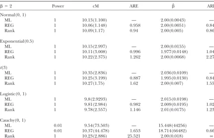
TABLE 1
Comparison of parametric and nonparametric methods (20 cM)
 ⫽2 Power cM ARE ˆ ARE
Normal(0, 1)
ML 1 10.13(1.100) — 2.00(0.0043) —
REG 1 10.06(1.148) 0.958 2.00(0.0051) 0.843
Rank 1 10.09(1.17) 0.94 2.00(0.005) 0.86
Exponential(0.5)
ML 1 10.15(2.997) — 2.00(0.0155) —
REG 1 10.11(3.008) 0.996 1.977(0.0148) 1.047
Rank 1 10.22(2.375) 1.262 2.00(0.0068) 2.279
t(3)
ML 1 10.35(2.836) — 2.036(0.0109) —
REG 1 10.25(3.199) 0.887 1.995(0.0130) 0.840
Rank 1 10.27(1.75) 1.62 2.00(0.007) 1.557
Logistic(0, 1)
ML 1 9.8(2.9293) — 2.015(0.0198) —
REG 1 9.81(2.984) 0.982 2.009(0.0195) 1.020
Rank 1 9.78(2.557) 1.146 2.01(0.0175) 1.236
Cauchy(0, 1)
ML 0.01 9.54(73.503) — 15.448(44256) —
REG 0.01 10.37(44.478) 1.653 18.714(66482) 0.666
Rank 1 10.23(2.886) 25.521 2.00(0.018) ∞
Tables 1–4 show the mean estimate of the QTL location (cM) and its gene effect (), with the empirical variances of the estimates over replicates in parentheses. ARE is the estimated asymptotic relative efficiency of regression analysis or rank-based methodvs. the ML method and is defined as var(ML)/var(REG)or var(ML)/ var(Rank).
with E(Xi|flanking markers), we obtain the rank test of. It can be shown that, for a given distribution, the
deviation goes to 0 as  goes to 0 or as the flanking statistic equivalent to the one inKruglyakandLander
(1995). Note that instead of testing H0directly, here we marker distance goes to 0. Thus we expect the estimator ˆ to work well in QTL analysis if either there is a rela-instead testM1 ⫽ M2 ⫽. . . ⫽ MK. Usually,K is much
greater than the number of underlying distributions. tively dense map (e.g.,⬍20 cM, a common scenario of current genetic studies) or the QTL effect is relatively For example, in the backcross population, we are
inter-ested in testing the difference between the two compo- small. Efficiency is of less concern when the QTL effect is nent distributions in the mixture model. In essence, we large than when it is small. In QTL mapping of complex test for differences among the four mixtures,Mk,k⫽ traits, an individual QTL usually has small effect. For
1, . . . , 4. Theoretically, it is unclear whether the relative these reasons, we believe and our simulations as well efficiency of the rank sum testvs. thet-test [or, equiva- show that the rank sum-based estimators are practically lently the likelihood-ratio test (LRT)] in linear regres- useful alternatives to the least-squares estimators from sion still holds in this setting. However, we expect that Haley and Knott’s regression interval mapping. the rank sum test performs better under most circum- The following are some properties ofˆ. To emphasize stances when data are nonnormal, which we investigate thatˆ depends onY⫽{Yi}, we rewriteˆ asˆ(Y). From
by simulations. the definition ofˆ, it is not difficult to show that, for The estimation ofis more problematic than that for anyb僆R,
simple linear regression. In traditional linear regression,
E{L()}⫽0. Thus the estimatorˆ is consistent. How- i. ˆ(Y)⫽ ˆ(Y⫹b)⫽defˆ(Y1⫹b, . . . ,Yn⫹b), and ever, due to the mixture structure of QTL data, we can ii. ˆ(Y)⫽ ⫺ˆ(⫺Y).
show thatE{L()} does not generally equal 0 whenXiis
substituted by its conditional expectation. A theoretical In words, i indicates that adding a constant to the data has no effect on the estimator of QTL effect. Property ii formula ofE{L()} indicates that the magnitude of the
deviation from 0 depends on the underlying distribu- says that if the data are multiplied by⫺1, the estimator has an opposite sign.
Normal(0, 1)
ML 1 10.18(2.412) — 1.00(0.0046) —
REG 1 10.24(2.689) 0.897 0.999(0.0051) 0.902
Rank 1 10.20(2.444) 0.987 1.00(0.0054) 0.852
Exponential(0.5)
ML 1 10.06(12.036) — 1.00(0.0172) —
REG 1 9.94(12.622) 0.954 0.999(0.018) 0.956
Rank 1 9.96(6.60) 1.824 1.00(0.0072) 2.389
t(3)
ML 1 10.43(8.51) — 1.00(0.0115) —
REG 1 10.530(6.817) 1.248 1.00(0.014) 0.821
Rank 1 10.32(4.038) 2.107 1.00(0.0075) 1.533
Logistic(0, 1)
ML 1 9.99(8.172) — 0.997(0.0167) —
REG 1 10.03(7.848) 1.041 0.999(0.0163) 1.020
Rank 1 9.86(7.031) 1.162 0.999(0.0153) 1.091
Cauchy(0, 1)
ML 0 9.66(78.53) — 5.011(1187) —
REG 0 9.09(46.265) 1.697 5.842(1698) 0.699
Rank 1 10.89(8.766) 8.958 1.00(0.017) ∞
Extensions:Next we extend the methods to any other 10 cM with simulated QTL at 5 cM or located at 0 and 20 cM with simulated QTL at 10 cM, respectively. The cross derived from two inbred lines, such as F2. In
gen-eral, the model can be expressed as P(Yi ⬍ y|Xi) ⫽ setups are similar to those inXu(1995). The QTL effect
is either 1 or 2. Standard normal, exponential(0.5),
F(y⫺Xi⬘), where ⫽(a,d)⬘andXi⫽(X1,i,X2,i)⬘. The
covariates t(3), standard logistic, and standard Cauchy are used as error distributions. One hundred simulations were
X1,i ⫽ ⫺1, 0, or 1 if individuali has QTL genotypeqq,
conducted for each combination with sample sizen⫽ qQ, orQQ, and
1000. The average values and corresponding standard
X2,i⫽1 (or 0) if individualihas QTL genotype qQ(or
errors of estimated QTL position, QTL effect from para-else)
metric interval mapping (ML), and nonparametric Wil-coxon rank sum interval mapping (Rank) are given in correspond to the additive and dominance genetic
ef-fects, a and d, respectively. In regression mapping, if Tables 1–4. As a comparison, we also run the regression analysis (REG) of Haley and Knott (1992) and the the unknown Xj,i’s are replaced by their conditional
expectationsE(Xj,i|flanking markers), then the estima- results are given in Table 1.
The estimates of QTL position and effect from the torˆ can be derived as described inrank-based
meth-odsfor multiple regression without any modifications. REG and the ML methods are very similar not only for normal data, which is consistent withHaleyandKnott
The methods may also be adapted to map multiple
QTL (Kaoet al. 1999) or to more complicated designs (1992) and with Xu (1995), but also for nonnormal data. Note that the nonparametric test and estimate involving more than two inbred lines (Liu and Zeng
2000) by changing the dimension of. Of course, the generally are much more efficient than the parametric versions when data are not normally distributed. There efficiency may be low if the dimension of  is large.
This requires further investigation. is a modest loss of efficiency with normal data, which agrees with theory for simple linear regression. The marker distances and the magnitude of the QTL effect
NUMERICAL STUDIES
do not seem to have a large impact on the relative efficiencies of the estimators.
Simulations were conducted to study the behavior of
Zandˆ in a backcross population. For simplicity, only To estimate the power, the rank test statisticZis first transformed to LODR ⫽ {2 log(10)}⫺1Z2 and the test
one chromosomal segment flanked by two markers is
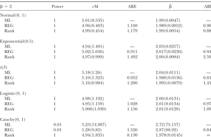
TABLE 3
Comparison of parametric and nonparametric methods (10 cM)
 ⫽2 Power cM ARE ˆ ARE
Normal(0, 1)
ML 1 5.01(0.535) — 1.99(0.0047) —
REG 1 4.96(0.483) 1.108 1.989(0.0052) 0.905
Rank 1 4.99(0.454) 1.179 1.99(0.0054) 0.884
Exponential(0.5)
ML 1 4.94(1.491) — 2.03(0.0217) —
REG 1 5.02(1.636) 0.911 2.017(0.0230) 0.945
Rank 1 4.97(0.999) 1.492 2.00(0.0084) 2.592
t(3)
ML 1 5.18(1.26) — 2.04(0.0111) —
REG 1 5.10(1.323) 0.952 1.988(0.0136) 0.818
Rank 1 5.16(0.984) 1.280 1.995(0.0079) 1.414
Logistic(0, 1)
ML 1 4.98(1.192) — 2.00(0.0131) —
REG 1 4.95(1.159) 1.028 2.01(0.0134) 0.973
Rank 1 5.000(1.030) 1.156 2.01(0.0120) 1.090
Cauchy(0, 1)
ML 0.01 5.23(14.987) — 2.72(75.157) —
REG 0.01 5.28(9.82) 1.526 2.87(88.92) 0.845
Rank 1 4.94(1.835) 8.130 1.978(0.0145) ∞
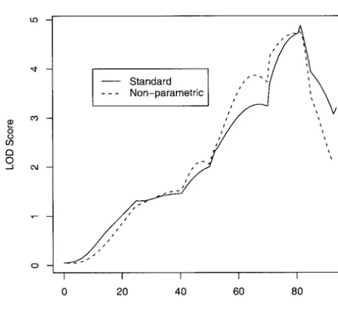
LOD score. We then take threshold 3 for the LOD position although the LOD curves are slightly different, which will result in some slightly different confidence scores, which is recommended in practical genome-wide
QTL analysis (see also Kruglyak and Lander 1995 intervals of the putative QTL locus by the conventional 1-LOD drop method. The additive and dominance esti-for analytic genome-wide threshold calculations). The
power is calculated as the proportion of significant tests mators are 0.262 and 0.059, respectively, from standard interval mapping and are 0.257 and 0.038, respectively, from 100 simulated data sets. For the extreme case
where data are Cauchy distributed, there is no power based on our method. To assess whether the differences between the two methods are significant or not, 1000 to detect the QTL by ML or REG interval mapping while
Rank interval mapping does have power. bootstraps are performed. We restrict our analysis within chromosome 1. From our method, the 95% confidence To further demonstrate the method, we consider the
data on the time to death following infection withListeria interval (CI) of the QTL locus is (50 cM, 84 cM). The mean of the additive effect is 0.247 with standard error
monocytogenesof 116 F2mice from an intercross between
the BALB/cByJ and C57BL/6ByJ strains (Boyartchuket 0.077 and the mean of the dominant effect is 0.055 with standard error 0.122. Similarly, from standard interval
al.2001). The histograms of the log time to death of
the nonsurvivors are given in Figure 1. Roughly 30% of mapping, we get the 95% CI of the QTL locus as (51 cM, 92 cM). The mean of the additive effect is 0.268 mice survive beyond 264 days. From the histogram it is
hard to justify that the log time to death of the nonsurvi- with standard error 0.071 and the mean of the dominant effect is 0.0284 with standard error 0.122. In all, the vors is normally distributed. Broman (2003) applied
four different methods, including both the standard nonparametric QTL locus estimator is relatively more efficient than the parametric estimator and our nonpar-interval mapping and nonparametric nonpar-interval mapping,
to this data set and showed that the locus on chromo- ametric analysis confirms the results ofBroman(2003). some 1 appears to have effect only on the average time
to death among the nonsurvivors. For this reason, our
CONCLUSION AND REMARKS
analysis is restricted on chromosome 1 for those
nonsur-vivors. In this article, traditional rank-based estimators for linear regression have been adapted to analyze quantita-The LOD scores obtained by standard interval
map-ping and the nonparametric interval mapmap-ping with the tive traits. The new method has been shown to be very similar to Haley and Knott’s regression interval mapping log time to death are plotted in Figure 2. It is clear that
Normal(0, 1)
ML 1 4.98(1.252) — 0.996(0.0039) —
REG 1 4.96(1.17) 0.986 0.996(0.0044) 0.885
Rank 1 4.96(1.19) 1.052 0.997(0.0046) 0.837
Exponential(0.5)
ML 1 5.03(4.252) — 1.00(0.018) —
REG 1 5.09(3.962) 1.073 1.00(0.0184) 0.980
Rank 1 5.09(2.26) 1.881 1.00(0.0064) 2.830
t(3)
ML 1 4.97(2.999) — 1.00(0.016) —
REG 1 4.92(2.80) 1.071 1.00(0.0161) 0.996
Rank 1 4.96(1.594) 1.881 0.993(0.0096) 1.667
Logistic(0, 1)
ML 1 5.12(3.581) — 0.993(0.0114) —
REG 1 5.07(3.157) 1.135 0.998(0.0116) 0.979
Rank 1 5.14(2.889) 1.239 0.996(0.0104) 1.096
Cauchy(0, 1)
ML 0 5.49(15.543) — 0.442(61.51) —
REG 0 5.34(10.69) 1.454 0.396(68.26) 0.901
Rank 1 4.88(3.238) 4.800 0.991(0.0146) ∞
for nonnormal data. Our simulations indicate that the based on one QTL model. We believe the nonparamet-ric model is very likely to produce ghost QTL as the normal likelihood-ratio-based interval mapping is
usu-ally unbiased, even when the data are nonnormal, but parametric method does when two QTL are close to each other and multiple nonparametric QTL mapping may have very low efficiency. All our simulations are
is needed.
In genetic studies of quantitative traits, adapting
rank-Figure1.—Histogram of log 2(survival time), following in-fection withListeria monocytogenesof 85 nonsurvival mice out
of a total of 116 mice. The remaining 31 mice recovered from Figure2.—LOD score curves from standard interval map-ping (solid line) and nonparametric interval mapmap-ping (dashed the infection and survived to the end of experiment, 264 hr
Boyartchuk, V. L., K. W. Broman, R. E. Mosher, S. E. F. Dorazio,
based methodologies is complicated because genetic
M. N. Starnbach et al., 2001 Multigenic control of Listeria
markers are observed only at known loci and the QTL monocytogenes susceptibility in mice. Nat. Genet.27:259–260.
Broman, K. W., 2003 Mapping quantitative trait loci in the case of
genotypes are usually unknown. Thus, the trait data
a spike in the phenotype distribution. Genetics163:1169–1175.
arise from discrete mixtures of unknown distributions.
Draper, N. R., and H.Smith, 1998 Applied Regression Analysis, Ed.
The mixture structure of the data may distort certain 3. John Wiley & Sons, New York.
Drinkwater, N. R., 1997 Qlink Documentation.McArdle Laboratory
properties of the underlying error distributions. For
for Cancer Research, University of Wisconsin, Madison, WI.
example, F may be unimodal even though the QTL
Drinkwater, N. R., andJ. H. Klotz, 1981 Statistical methods for
data may not be. This means that the rank test in QTL the analysis of tumor multiplicity data. Cancer Res.41:113–119.
Hajek, J., 1968 Asymptotic normality of simple linear rank statistics
mapping may have properties that differ from those for
under alternatives. Ann. Math. Stat.39:325–346.
the rank test in linear regression.
Hajek, J., andZ. Sidak, 1967 Theory of Rank Tests. Academic Press,
As explained innonparametric interval mapping, New York/London.
Haley, C. S., andS. A. Knott, 1992 A simple regression method for
the rank-based parameter estimate ˆ is not generally
mapping quantitative traits in line crosses using flanking markers.
unbiased with QTL data because the unknown
regres-Heredity69:315–324.
sorsXiare replaced by their expectations. On the basis Jansen, R. C., andP. Stam, 1994 High resolution of quantitative
traits into multiple loci via interval mapping. Genetics136:1447–
of the theory of general estimating equations (Liang
1455.
andZeger1986), one may show that the estimators of
Kao, C. H., Z-B. ZengandR. D. Teasdale, 1999 Multiple interval
genetic effects fromHaleyandKnott’s (1992) regres- mapping for quantitative trait loci. Genetics152:1203–1216.
Kraft, C. H., andC. van Eeden, 1972 Linearized rank estimates
sion method are unbiased, although the variances of the
and signed rank estimates for the general linear hypothesis. Ann.
estimators may be larger than those from the
Hodges-Math. Stat.43:42–57.
Lehmann estimators. While the rank-based estimators Kruglyak, L., andE. S. Lander, 1995 A nonparametric approach
for mapping quantitative trait loci. Genetics139:1421–1428.
are theoretically biased, in simulations, the bias is
negli-Lander, E. S., andD. Botstein, 1989 Mapping Mendelian factors
gible when compared with the regression and
maxi-underlying quantitative traits using RFLP linkage maps. Genetics
mum-likelihood methods. 121:185–199.
Liang, K. Y., andS. L. Zeger, 1986 Longitudinal data analysis using
The computation of ˆ usually is complicated if the
generalized linear models. Biometrika73:13–22.
dimension ofis⬎1 and requires some iterative
proce-Lincoln, S. E., M. J. DalyandE. S. Lander, 1993 A Tutorial and
dures.Kraftandvan Eeden(1972) proposed an easy Reference Manual for MAPMAKER/QTL. Whitehead Institute for
Biometrical Research.
one-step modification of the least-squares estimator of
Liu, Y., andZ-B. Zeng, 2000 A general mixture model approach
to approximateˆ. We may use this one-step
modifica-for mapping quantitative trait loci from diverse cross designs
tion if the calculation ofˆ is too complicated, involving multiple inbred lines. Genet. Res.75:345–355.
Morton, N. E., 1984 Trials of segregation analysis by deterministic
ˆ ⬇˜ ⫹A⫺1
n [C⫺1n Ln(˜)], (3) and macro simulation, pp. 83–107 inHuman Population Genetics: The Pittsburgh Symposium, edited by A.Chakravarti. Van
Nos-where˜ is the least-squares estimator of, and for any trand Reinhold, New York.
Puri, M. L., andP. K. Sen, 1985 Nonparametric Methods in General d僆p,
Linear Models. John Wiley & Sons, New York.
Sax, K., 1923 The association of size differences with seed-coat
pat-An⫽
冢
[Ln(˜)⫺Ln(˜⫺n⫺1/2d)]⬘[Ln(˜)⫺Ln(˜⫺n⫺1/2d)]
(d⬘C2
nd)/n2
冣
1/2
. tern and pigmentation inPhaseolus vulgaris.Genetics8:552–560. Xu, S., 1995 A comment on the simple regression method for
inter-val mapping. Genetics141:1657–1659.
Zeng, Z-B., 1993 Theoretical basis of separation of multiple linked gene effects on mapping quantitative trait loci. Proc. Natl. Acad. Sci. USA90:10972–10976.
LITERATURE CITED
Zeng, Z-B., 1994 Precision mapping of quantitative traits loci. Genet-Basten, C. J., B. S. WeirandZ-B. Zeng, 1997 QTL Cartographer: A ics136:1457–1468.
Reference Manual and Tutorial for QTL Mapping.Department of