Performance of error control coding techniques for wireless ATM

(1)

Performance

of

Error Control Coding

Techniques

for

Wireless ATM

Peter R. Denz

Arne A. Nilsson

Center for Advanced Computing and Communication

Department of Electrical and Computer Engineering

North Carolina State University

(2)

Abstract

With recent advances in the area of wireless communications, mobile communications are becoming more and more prevalent. At the same time, wired networks are evolving toward the use of ATM as a transport mechanism because of its support of bandwidth-intensive applications, its ability to carry varying media types, and its ability to provide the application with a guaranteed quality of service. In the future, we would like to provide a ubiquitous telecommunications network which merges these concepts. This new wireless ATM concept brings with it many new challenges that must be overcome for the network to be a success. ATM was designed with the assumption that the network medium has a very low bit error rate, the users do not move, and the physical medium has a very high bandwidth. Wireless communications, on the other hand, suffers from a very high bit error rate, the users are mobile, and the bandwidth available is relatively low. In this paper, we focus on the problem of reducing the effects of the high bit error rate on the data transmission. We present a simulator which can be used to study the effects of various coding techniques on the overall system bit error rate. Among these coding techniques are convolutional coding, interleaving, fragmentation, and puncturing. We show that convolutional coding, along with interleaving or fragmentation, improves transmission reliability over the bursty error channel.

I. Introduction

In the future, ATM has the potential of becoming ubiquitous on all computer platforms. Thus, to avoid the problem of protocol conversion, it is important for it to be provided on wireless systems. The wireless ATM should be designed in such a way that seamless integration can be made with wired ATM systems. [5]

The combining of broadband networks and wireless networks introduces a set of challenges due to the two fundamental differences between the networks (i.e., link characteristics and mobility).

Broadband networks have a very high transmission rate and very low bit error rate. Wireless networks, on the other hand, are characterized by a relatively low transmission rate and relatively high bit error rate. Wireless links suffer from multipath fading resulting in a varying bit error rate. In broadband networks, the user-network interface (UNI) is fixed; whereas it is variable in a wireless setting due to user mobility. The mobility has brought about the need to redesign things such as virtual path routing, call admission control, resource allocation, and so forth while the noisy wireless channel has brought about the need for increased error control. [10]

Wireless communications must deal with more interferences from the surrounding environment in the form of line noise and echoes. The field strength is highly dependent on the physical environment: geographical surroundings, distance from the base station, building structure materials, etc. Interferences typically cause bursts of transmission errors or even disconnection in the worst case. Errors are often increased if the mobile station is actually moving (e.g., in a car) which may lead to changes in coverage area causing at least a temporary disconnection. [2] Wireless channels suffer from long-term fading and short-term fading. Long-term fading refers to conditions when the average signal changes slowly over time whereas short-term fading refers to quick fluctuations of the signal due to reflection, scattering, and diffraction. Both of these types of fading have an impact on the bit error rate of the wireless link. [10] Thus, wireless communication suffers from low bandwidth, high error rate, and frequent disconnections. These, in turn, increase the network latency due to retransmissions, time outs, and error processing. [6] Power requirements in the handset have a significant effect on the achievable bit-rate. For example, in a small cell, 1.5 to 2 Mbps may be possible, whereas in a large cell only a few hundred Kbps may be possible. [3] To boost the reliability of the actual wireless link, antenna diversity techniques should be used to protect against multipath fading and interference. [1]

(3)

Network call processing functions must be involved to set up a new route using the new access point and to ensure that the QoS is at an acceptable level for the current mobile and all mobiles that share the new access point. [10] During the period of the handoff the user may see a degradation of channel quality. It may be beneficial to implement a stronger error control protocol to reduce the channel noise incurred by handoffs.

Some research has already been done to attempt to find viable solutions to some of the problems hindering wireless ATM. Karol, et al. presents a scheme to handle the mobility aspect of the wireless end station. This scheme, called a connection tree, exploits statistical multiplexing to prevent the overload of a base station. [9] Eng, et al. proposes the BAHAMA (A Broadband Ad-hoc wireless ATM LAN) scheme which solves the mobility problem by associating each mobile with a “home” base station and a series of forwarding pointers until the current mobile location is reached. [5] Several wireless-ATM channel access protocols have been proposed, including the DQRUMA protocol in [9]. Work still needs to be done to reduce the high bit error rate of the wireless channel. In this paper, we will present results of a

simulator in which error control coding was added to a wireless ATM network scenario.

In order to avoid having to provide protocol conversion required if this error correction coding were placed at the ATM layer, we placed the coding in the AAL on the end stations. Forward error correction (FEC) implementation at the SAR layer lends itself to the use of block coding due to the fixed size of ATM cells (the cell size specifies the block length). On the other hand, FEC implementation at the convergence sublayer lends itself to the use of convolutional coding due to the long streams of data. [4] We chose to implement convolutional coding at the CS sublayer.

After the data is run through the convolutional encoder, the encoded message gets split up and placed into ATM cells. In order for a series of damaged bits or a lost cell to be properly reconstructed at the receiver, sufficiently long streams of correctly received cells must be received before and after the damaged bits or lost cell. These streams are known as the guard space and contain the redundancy needed to reconstruct the missing cell. [4]

The problem with this scheme is that errors in wireless networks typically occur in bursts, thus requiring an ever-increasing guard space to properly recover from the loss. The number of consecutive packets lost can be significantly reduced by interleaving the packet streams as they leave the sender. This will result in a smaller guard space being required and, in turn, an increase in the error correction abilities of the scheme. [4]

II. Simulator Description

The Wireless ATM Handoff Simulator is a simulation engine that can be used to study the effects of various coding techniques on a bursty error channel. Among the user-modifiable parameters are: channel model parameters, convolutional code, puncturing matrix, data interleaver, and various time and frame size distributions (packet arrival, handoff time, inter-handoff time, frame length, etc.).

(4)

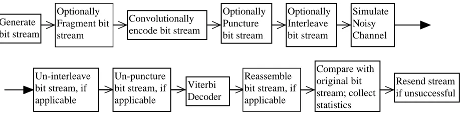
retransmitted packets, the frame length for successful packets, and the number of retransmissions required by each frame. The block diagram in figure 1 is a graphical representation of the tasks modeled by the simulator.

Figure 1: Simulator Block Diagram

The simulator continuously oscillates between two modes of operation—normal (non-handoff) mode and handoff mode. Each of these modes of operation has different channel characteristics which are modeled in the simulator (i.e., during handoff mode, error bursts tend to occur more frequently and may persist for a longer duration). The simulator allows different levels of puncturing to be applied for each of these modes of operation. During the transmission of one long packet, the simulator may transition back and forth between handoff and non-handoff modes of operation. In this case, the channel parameters will change with each transition, but the puncturing level used will remain as the one used during the mode in which packet transmission had begun.

Interleaving

The interleaver successively places the input bit stream into a (n x n) matrix row-wise and puts these bits out onto the channel in a column-wise fashion. The following example shows the results of the first interleaving matrix on a bit stream of length n using a square interleaving matrix of size 3. Here the bit stream (b1, b2, b3, …, bn) is fed to the interleaver and leaves the interleaver as the sequence (b1, b4, b7, b2, b5, b8, b3, b6, b9, …).

(b1, b2, b3, …, bn) à

b

1 2 3

4 5 6

7 8 9













à (b1, b4, b7, b2, b5, b8, b3, b6, b9, …)

Within a single interleaving matrix, (bi, bi+1) of the input stream are separated by n in the output stream when bi does not appear in the rightmost matrix column (i.e., when i is not a multiple of n). When bi does fall in the rightmost matrix column, (bi, bi+1) are separated by (2n - 1). However, the last bit of one interleaving matrix and the first bit of the next interleaving matrix remain adjacent before and after interleaving using this scheme. A more powerful interleaving scheme may be used to eliminate this.

In the case of a square interleaving matrix, un-interleaving is merely done by invoking the interleaver a second time. Continuing with the previous example,

Generate bit stream

Convolutionally encode bit stream

Optionally Interleave bit stream Optionally Puncture bit stream Simulate Noisy Channel Un-interleave bit stream, if applicable

(5)

(b1, b4, b7, b2, b5, b8, b3, b6, b9, …) à

b

1 4 7

2 5 8

3 6 9













à (b1, b2, b3, b4, b5, b6, b7, b8, b9, …).

So, our original bit stream is successfully regenerated.

In the case where the total interleaver matrix capacity is greater than the remaining bit stream size, the bit stream is padded to fill out the interleaver and simplify processing at the destination.

The block diagram of figure 1 illustrates the placement of the interleaver/un-interleaver function into the simulator. The convolutionally encoded bits are fed into the interleaver and spread apart prior to entering the channel. On the channel, the bit stream suffers the effects of a bursty error channel. At the destination, the bits are properly reordered, effectively spreading out the error bursts. Since a

convolutional code requires a number of correctly transmitted “guard” bits around each erroneous bit, the spreading should aid in the correction of the burst errors. Finally, the bit stream enters the decoder which attempts to correct errors in the stream.

Fragmentation

The simulator assumes that packets are variable length from the CS sublayer of the AAL (prior to segmentation). Since long packets tend to suffer more errors than short packets on the channel,

fragmentation may be used. By fragmenting the large packet into fixed size small blocks, we effectively have convolutional encoding on fixed blocks. By convolutionally encoding small fixed blocks, we will ideally be able to have a lower probability of a retransmission. This comes at a cost, though, as there is a certain amount of overhead that is attached to each encoded block (the bits to flush the buffer). In the original long packet, this overhead appears only once, but for the encoded fragments, it appears once for each fragment. The following figure illustrates both a long encoded packet with a small amount of overhead and fragmented packet with convolutionally encoded blocks.

Long Encoded Packet (no fragmentation)

Encoded Packet Fragments Showing increased overhead

Figure 2: Fragmentation Example

Each convolutionally encoded segment requires the addition of M trailing bits to flush the encoder memory (where M is the memory order of the encoder). If the original long frame is of length A and the fragments are of length N, then the resulting frame with memory flush bits (overhead) is of length

A

N

M

A









+

. An interesting problem is to find the optimal value of N such that the increased coding

efficiency nicely balances the increased overhead of this scheme. Long Packet

(6)

Puncturing

Puncturing is the process of systematically deleting bits from the output stream of a low-rate encoder in order to reduce the amount of data to be transmitted, thus forming a high-rate code. The bits are deleted according to a perforation matrix. The new high-rate code is dependent on the low-rate original code in addition to the perforation matrix. For instance, if the output of the encoder is

represented by “1234567890”, and the puncturing matrix

1 1

1 0









_



were used, then the resulting

“punctured” stream would be “12356790” since the matrix specifies that each fourth bit is to be deleted. Puncturing may be employed to dynamically change the coding rate during transitions between handoff and non-handoff modes of operation, to account for the differing channel characteristics. Rate-compatible punctured convolution codes (RCPC) allow the error correction capability to adapt to the channel quality while using the same encoder/decoder pair at all times. [8] Puncturing in the simulator can be specified independently for both the handoff and non-handoff modes.

Bursty Channel Model

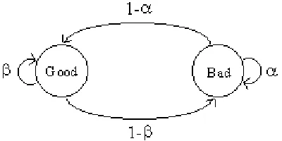
The Gilbert Channel Model is a channel in which bit errors occur in distinct bursts. The model consists of two states—a good and a bad state (refer to the Gilbert Model state diagram shown in figure 3). No errors occur during a good state, but errors can occur in the bad state. The probability of transitions from state to state is shown on the diagram. In this simulator, an error occurs during the bad state with probability ½. [7]

Figure 3: Gilbert Channel Model

We can now calculate the overall probability of being in a good or bad state which will in turn give us an idea of the expected error burst length and the expected good bit stream length.

P Good

[

]

=

−

+

−

1

1 β

α

β

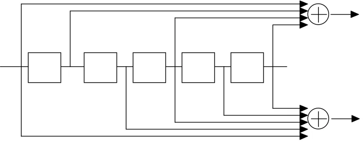
Convolutional Encoder/Viterbi Decoder

(7)

Figure 4: (2, 1, 5) Convolutional Encoder

III. Simulation Results

General Comments

We ran many simulations varying one input parameter for each series. This way, the effects of this particular input parameter can be seen on all of the various output statistics. The graphs with multiple lines and no legend have the 95% confidence interval shown. The simulations seem to reach steady state since the confidence interval follows the mean very closely.

In general, it does not make sense to view the frame length for successful packets and frame length for unsuccessful packets parameters across many simulations. In the simulations I have run, the frame length corresponded closely to the expected packet length, as it should since we keep retransmitting failed packets until they finally succeed. In any particular simulation run, the average frame length for unsuccessful packets is always larger than the average frame length for successful packets. This is intuitive as longer frames have a greater probability of not being properly corrected by the Viterbi decoder.

Since packet sizes follow a truncated exponential distribution, and since error coding is most effective on smaller packet lengths, we will see packets less than a certain threshold in length get transmitted successfully; whereas packets larger than this threshold require retransmission.

Simulation Run Series

Among the parameters that were varied in the simulation runs include the probability to start a burst and the probability to remain in a burst for both the handoff and the non-handoff (regular) modes of operation, the puncturing mask used in either mode of operation, the interleaver size, and the

fragmentation size. The following is a list of the various simulation run series that were analyzed:

dn Series Vary the probability of starting an error burst in non-handoff mode

dns Series Vary the probability of staying in an error burst during non-handoff mode

dh Series Vary the probability of starting an error burst in handoff mode

dhs Series Vary the probability of remaining in an error burst during handoff mode

dcin Series Same as dn series, but with an interleaver of size 10 used

di Series Vary interleaver size

dcfn Series Vary the probability of starting an error burst in non-handoff mode with fragmentation

size equal to 50.

(8)

dph Series Vary puncturing matrix in handoff mode

ddht Series Modify the handoff time distribution

Channel Parameters

In each of these series, the effects of the Gilbert Model state transition variables are studied for both the handoff and non-handoff modes of operation. For these simulation series, the simulator mode transitions follow a uniform distribution with variables having the following values:

MIN_INTER_HANDOFF_TIME = 30 MAX_INTER_HANDOFF_TIME = 40 MIN_HANDOFF_TIME = 1

MAX_HANDOFF_TIME = 10

Thus, the expected handoff time is 5.5 and the expected inter-handoff time (i.e., time spent in non-handoff mode) is 35. Therefore because so much more time is expected to be spent in non-handoff mode than in handoff mode, changes to parameters that occur only in non-handoff mode are expected to have a much stronger influence on the simulation results compared to changes to parameters in handoff mode. The simulation results indeed support this expected behavior.

Vary the Probability of Starting an Error Burst

In the dn and dh series, we vary the probability of entering a bad state in the Gilbert model while in non-handoff mode and handoff mode, respectively. Since the non-handoff mode is long compared to the handoff mode, the affect of the modification of this variable has a much stronger influence on the overall performance than the modification of the variable in the handoff mode. Intuitively, as the probability of starting a burst increases, so does the time until successful transmission, the number of retransmissions per frame, and the probability of frame retransmission.

P[Start Burst] vs Mean Time until Successful Transmission in Handoff and Non-Handoff Modes

0 50 100 150 200 250 300 350 400

0 0.01 0.02 0.03 0.04 0.05 0.06 0.07

P[Start Burst]

M

ean Time until Successfu

l

Transmission

Non-Handoff Mode Handoff Mode

(9)

P[Start Burst] vs Mean Number of Retransmissions for Handoff and Non-Handoff Modes

0 1 2 3 4 5 6 7

0 0.01 0.02 0.03 0.04 0.05 0.06 0.07

P[Start Burst]

Mean Number o

f

R

etransmission

s

Figure 6: DN and DH Series, Mean Number of Retransmissions Per Frame

P[Start Burst] vs Probability of Frame Retransmission for Handoff and Non-Handoff Modes

0 0.1 0.2 0.3 0.4 0.5 0.6 0.7 0.8 0.9 1

0 0.01 0.02 0.03 0.04 0.05 0.06 0.07

P[Start Burst]

P

robability of Fram

e

Retransmission

Figure 7: DN and DH Series, Probability of Frame Retransmission

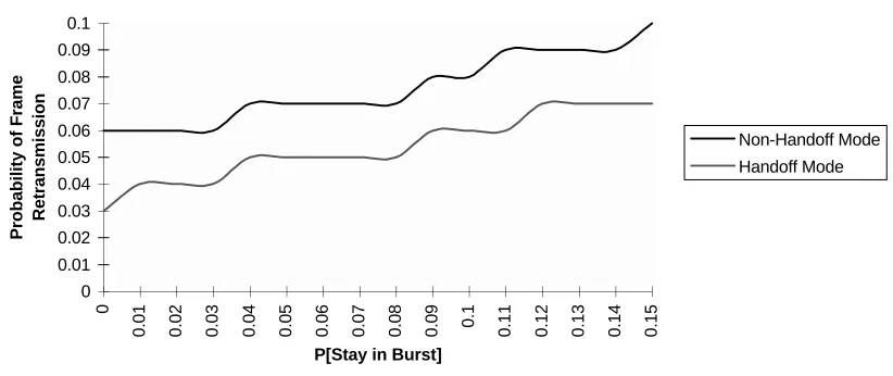
Vary the Probability of Remaining in an Error Burst

As we vary the probability of remaining in an error burst during the non-handoff and handoff modes of operation, in the dns and dhs series, respectively, all of the statistics (the time for successful transmission, the number of retransmissions required per frame, and the probability of frame

(10)

P[Stay in Burst] vs Mean Time Until Successful Transmission, Handoff and Non-Handoff Modes

22 23 24 25 26 27 28

0

0.01 0.02 0.03 0.04 0.05 0.06 0.07 0.08 0.09 0.1 0.11 0.12 0.13 0.14 0.15

P[Stay in Burst]

M

l

Transmission

Figure 8: DNS and DHS Series, Mean Time Until Successful Transmission

P[Stay in Burst] vs Mean Number of Retransmissions, Handoff and Non-Handoff Mode

0 0.02 0.04 0.06 0.08 0.1 0.12

0

0.01 0.02 0.03 0.04 0.05 0.06 0.07 0.08 0.09 0.1 0.11 0.12 0.13 0.14 0.15

Mean Number o

f

R

etransmission

s

(11)

P[Stay in Burst] vs Probability of Frame Retransmission

0 0.01 0.02 0.03 0.04 0.05 0.06 0.07 0.08 0.09 0.1

0

0.01 0.02 0.03 0.04 0.05 0.06 0.07 0.08 0.09 0.1 0.11 0.12 0.13 0.14 0.15

P

e

Retransmission

Figure 10: DNS and DHS Series, Probability of Frame Retransmission

Interleaving

(12)

P[Start Burst] vs Mean Time Until Successful Tranmission, Interleaving and No Interleaving

0 20 40 60 80 100 120 140 160 180

0 0.01 0.02 0.03 0.04 0.05 0.06

P[Start Burst]

M

ean Time Until Successfu

l

Transmission

No Interleaving Interleaving

Figure 11: DCIN Series, Mean Time Until Successful Transmission

P[Start Burst] vs Mean Number of Retransmissions, Interleaving and No Interleaving

0 0.5 1 1.5 2 2.5 3

0 0.01 0.02 0.03 0.04 0.05 0.06

P[Start Burst]

Mean Number o

f

R

etransmission

s

(13)

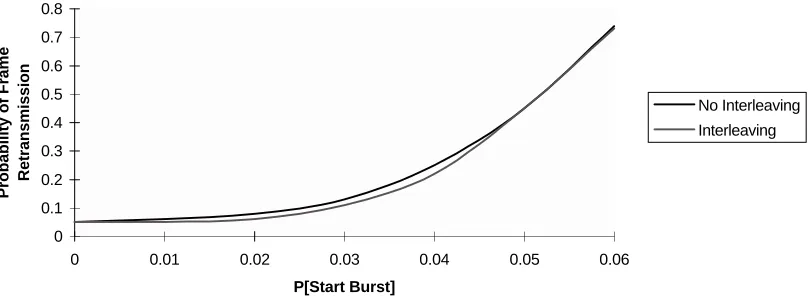
P[Start Burst] vs Probability of Frame Retransmission, Interleaving and No Interleaving

0 0.1 0.2 0.3 0.4 0.5 0.6 0.7 0.8

0 0.01 0.02 0.03 0.04 0.05 0.06

P[Start Burst]

P

e

Retransmission

Figure 13: DCIN Series, Probability of Frame Retransmission

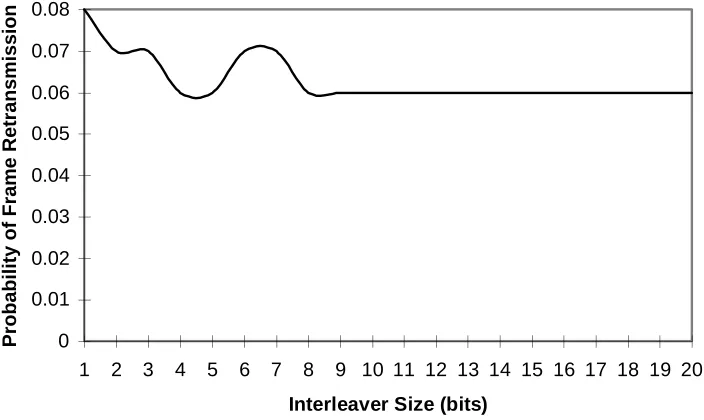
Varying Interleaver Size

In this series, the x-axis represents the size of the interleaver matrix (NOTE: x =1 is equivalent to no interleaving). We expect that as the interleaver gets larger, the error correction strength improves because adjacent bit positions of a burst are spread farther and farther apart.

(14)

Interleaver Size vs Mean Time Until Successful Transmission

24 24.5 25 25.5 26 26.5 27 27.5

1 2 3 4 5 6 7 8 9 10 11 12 13 14 15 16 17 18 19 20

Interleaver Size (bits)

M

ean Time until Successf

ul

Transmission

Figure 14: DI Series, Mean Time Until Successful Transmission

Interleaver Size vs Mean Number of Retransmissions Per

Frame

0 0.01 0.02 0.03 0.04 0.05 0.06 0.07 0.08 0.09 0.1

1 2 3 4 5 6 7 8 9 10 11 12 13 14 15 16 17 18 19 20

M

ean Number of Retransmission

s

Per Frame

(15)

Interleaver Size vs Probability of Frame Retransmission

0 0.01 0.02 0.03 0.04 0.05 0.06 0.07 0.08

1 2 3 4 5 6 7 8 9 10 11 12 13 14 15 16 17 18 19 20

P

robability of Frame Retransmissio

n

Figure 16: DI Series, Probability of Frame Retransmission

Fragmentation

The following graph compares the case of fragmentation (dcfn series) versus no fragmentation (dn series) when varying the probability of starting a burst during non-handoff mode. A fixed

(16)

P[Start Burst] vs Time Until Successful Transmission, Fragmentation and No Fragmentation

0 20 40 60 80 100 120 140 160 180

0 0.01 0.02 0.03 0.04 0.05 0.06

P[Start Burst]

M

l

Transmission

No Fragmentation Fragmentation

Figure 17: Comparison of DCFN and DN Series, Mean Time Until Successful Transmission

The following graph is a “zoom in” version of the previous graph showing that the lines actually cross because the fragmentation overhead requires more transmission time for very low probabilities of error.

Zoom in of P[Start Burst] vs Mean Time Until Successful Tranmission, Fragmentation and No Fragmentation

20 25 30 35 40 45

0 0.01 0.02 0.03 0.04

P[Start Burst]

M

l

Transmission

Figure 18: Closer Inspection of DCFN and DN Series, Mean Time Until Successful Transmission

(17)

P[Start Burst] vs Mean Number of Retransmissions, Fragmentation and No Fragmentation

0 0.5 1 1.5 2 2.5 3

0 0.01 0.02 0.03 0.04 0.05 0.06

P[Start Burst]

Mean Number o

f

R

etransmission

s

Figure 19: DCFN Series, Mean Number of Retransmissions Per Frame

P[Start Burst] vs Probability of Frame Retransmission, Fragmentation and No Fragmentation

0 0.1 0.2 0.3 0.4 0.5 0.6 0.7 0.8

0 0.01 0.02 0.03 0.04 0.05 0.06

P[Start Burst]

P

e

Retransmission

No Fragmenation Fragmentation

Figure 20: DCFN Series, Probability of Frame Retransmission

Punctured Convolutional Coding

Vary Puncturing Matrix used during non-handoff mode

(18)

time units handoff time), according to the input parameters, the overall effect of the non-handoff mode coding dwarfs the effect of the handoff mode coding. The data in all three graphs (mean time until successful transmission, probability of retransmission, and mean number of retransmissions per frame) is as we expect. A very “strong” puncturing matrix introduces many errors into the bit stream, reducing the effectiveness of the error correction coding. As the puncturing matrix “strength” is reduced (as the distance between punctured bits increases), the code tends to approach the performance of the use of no puncturing matrix.

1 = Rate 2/3 Puncturing Mask : 1 1 1 0 2 = Rate 3/5 Puncturing Mask : 1 1 1 1 1 0 3 = Rate 4/7 Puncturing Mask : 1 1 1 1 1 1 1 0 4 = Rate 5/9 Puncturing Mask : 1 1 1 1 1 1 1 1 1 0 5 = Rate 6/11 Puncturing Mask : 1 1 1 1 1 1 1 1 1 1 1 0 6 = Rate 7/13 Puncturing Mask : 1 1 1 1 1 1 1 1 1 1 1 1 1 0 7 = Rate 8/15 Puncturing Mask : 1 1 1 1 1 1 1 1 1 1 1 1 1 1 1 0 8 = Rate 9/17 Puncturing Mask : 1 1 1 1 1 1 1 1 1 1 1 1 1 1 1 1 1 0 9 = Rate 10/19 Puncturing Mask : 1 1 1 1 1 1 1 1 1 1 1 1 1 1 1 1 1 1 1 0 10 = Rate 11/21 Puncturing Mask : 1 1 1 1 1 1 1 1 1 1 1 1 1 1 1 1 1 1 1 1 1 0 11 = Rate 12/23 Puncturing Mask : 1 1 1 1 1 1 1 1 1 1 1 1 1 1 1 1 1 1 1 1 1 1 1 0 12 = No Puncturing Mask : 1

(19)

Puncturing Matrix vs Mean Time Until Successful

Transmission

0 100 200 300 400 500 600 700

1 2 3 4 5 6 7 8 9 10 11 12

Puncturing Matrix

M

ul

Transmission

Figure 22: DP Series, Mean Time Until Successful Transmission

Puncturing Matrix vs Mean Number of Retransmissions Per

Frame

0 2 4 6 8 10 12

1 2 3 4 5 6 7 8 9 10 11 12

Mean Number of

R

etransmissions Per Fram

e

(20)

Puncturing Matrix vs Probability of Frame Retransmission

0 0.1 0.2 0.3 0.4 0.5 0.6 0.7 0.8 0.9 1

1 2 3 4 5 6 7 8 9 10 11

Puncturing Matrix, Handoff mode

P

robability of Frame Retransmissio

n

Figure 24: DP Series, Probability of Frame Retransmission

Vary puncturing matrix in handoff mode.

Like the non-handoff mode puncturing series, the puncturing matrix is modified at each simulation run, but this time during the handoff mode. The leftmost point on the x-axis represents the strongest puncturing matrix. As we move to the right on the x-axis, the distance between punctured bits increases. Since the handoff mode occurs so much more infrequently than the handoff mode, the effect of the puncturing matrix on the overall simulation statistics is not as pronounced as the non-handoff case. The general trend, as expected, is for the time until successful transmission, the number of

(21)

Handoff Mode Puncturing Matrix vs Mean Time Until

Successful Transmission

0 5 10 15 20 25 30 35

1 2 3 4 5 6 7 8 9 10 11 12

M

l

Transmission

Figure 25: DPH Series, Mean Time Until Successful Transmission

Handoff Mode Puncturing Matrix vs Mean Number of

Retransmissions Required Per Frame

0 0.02 0.04 0.06 0.08 0.1 0.12 0.14 0.16 0.18

1 2 3 4 5 6 7 8 9 10 11 12

Mean Number of

R

etransmissions Required Pe

r

Frame

(22)

Handoff Mode Puncturing Matrix vs Probability of Frame

Retransmission

0 0.02 0.04 0.06 0.08 0.1 0.12 0.14 0.16

1 2 3 4 5 6 7 8 9 10 11 12

P

e

Retransmission

Figure 27: DPH Series, Probability of Frame Retransmission

Hand-off time distribution

In this series, labeled the ddht series, the handoff time, which follows a uniform distribution, is varied with the following (MIN_HANDOFF_TIME, MAX_HANDOFF_TIME) pairs:

X-axis (Min, Max)

0 (0, 0)

1 (0, 100)

2 (100, 200)

3 (200, 300)

...

i (100(i-1), 100i)

...

10 (900, 1000)

Since during the handoff mode, the channel is much more noisy than the non-handoff case, as we increase the time in the handoff, the time until successful transmission, the number of retransmissions per frame, and the probability of frame retransmission all increase. In this simulation series, the Gilbert channel characteristics are as follows:

NORMAL_PROB_START_BURST = 0.02 NORMAL_PROB_STAY_IN_BURST = 0.10 HANDOFF_PROB_START_BURST = 0.05 HANDOFF_PROB_STAY_IN_BURST = 0.18

(23)

Handoff Time Distribution vs Mean Time Until Successful

Tranmission

0 20 40 60 80 100 120 140 160 180 200

1 2 3 4 5 6 7 8 9 10 11

Hand-Off Time Distribution

M

ul

Transmission

Figure 28: DDHT Series, Mean Time Until Successful Transmission

Handoff Time Distribution vs Mean Number of

Retranmissions

0 0.2 0.4 0.6 0.8 1 1.2 1.4 1.6 1.8

1 2 3 4 5 6 7 8 9 10 11

M

ean Number of Retransmissio

ns

(24)

Handoff Time Distribution vs Probability of Frame

Retransmission

0 0.1 0.2 0.3 0.4 0.5 0.6 0.7

1 2 3 4 5 6 7 8 9 10 11

P

e

Retransmission

Figure 30: DDHT Series, Probability of Frame Retransmission

IV. Conclusion

In this paper, we have presented some of the results of the wireless-ATM error control simulator. A strong error correction code scheme will be essential to the functioning of a wireless-ATM protocol due to the high bit error rate of the underlying wireless channel. Convolutional coding is an ideal choice for the variable packet size of the CS-PDUs. As can be seen from the results of this simulator, some type of interleaving of the bit stream will be beneficial to increasing the error-correcting power of the

convolutional code. Fragmentation of the packets also results in much better error correction properties. Punctured convolutional coding is an attractive idea since it could dynamically vary the coding rate, adapting to changing channel characteristics; however, it is probably not appropriate in this scenario since it basically adds more errors to an already high error rate channel. Coding techniques used during the non-handoff mode of operation have a much stronger effect on overall system performance due to the relative time spent in the non-handoff and handoff mode states.

(25)

IV. References

[1] A.S. Acampora and M. Naghshineh. Control and Quality-of-Service Provisioning in High-Speed Microcellular Networks. IEEE Personal Communications, Second Quarter 1994, pp. 36-42. [2] T. Alanko, M. Kojo, H. Laamanen, M Liljeberg, M. Moilanen, and K. Raatikainen. Measured

Performance of Data Transmission Over Cellular Telephone Networks. Computer Communication Review, 24(4) pp. 24-44, October 1994.

[3] H. Armbruester. The Flexibility of ATM: Supporting Future Multimedia and Mobile Communications. IEEE Communications Magazine, February 1995, pp. 76-84.

[4] A. Dholakia, M.A. Vouk, and D.L. Bitzer. A Lost Cell Recovery Technique Using Convolutional Coding at the ATM Adaptation Layer in B-ISDN/ATM. In Proc. Fifth Intl. Conf. Data Comm. Sys. and Their Perf., Raleigh, NC, October 1993.

[5] K.Y. Eng, et al. BAHAMA: A Broadband Ad-Hoc Wireless ATM Local-Area Network. Proc. ICC’95 (1995) pp. 1216-1223.

[6] G.H. Forman, and J. Zahorjan. The Challenges of Mobile Computing. IEEE Computer. pp. 38-47. April 1994.

[7] E. N. Gilbert. Capacity of a Noise-Burst Channel. The Bell System Technical Journal. Pp. 1253-1265. September 1960.

[8] J. Hagenauer, N. Seshadri, and C.W. Sundberg. "The performance of rate- compatible punctured convolutional codes for digital mobile radio." IEEE Transactions on Communications, COM-38(7): 966-980, 1990.

[9] M.J. Karol, Z. Liu, and K.Y. Eng. An Efficient Demand-Assignment Multiple Access Protocol for Wireless Packet (ATM) Networks. Wireless Networks 1 (1995) pp. 267-279.