Computer-Aided Thermal Design Optimisation
Mohamed M. El-Awad
Associate Professor, Department of Engineering, Sohar College of Applied Sciences, Sohar, Oman
ABSTRACT: The aim of this paper is to demonstrate by means of relevant examples the usefulness of Excel as a tool for introducing computer-aided design optimisation to engineering students.The performance of thermal systems is strongly influenced by the cost of energy which constitutes a major part of their running cost.Thermal design, which must take into consideration operating costs as well as initial costs, offers good examples of design optimisation. Moreover, design optimisation of thermal systems can easilybe performed by using Excel. The examples considered in the paper deal with insulated conduits carrying hot or cold air with respect to initial and energy costs. Unlike analytical optimisation that can only be used for simple situations with a single design parameter, Excel can deal with thermal designs that involve multiple design factors and elaborate analytical models.
KEYWORDS: Thermal-fluid systems, design optimisation; Excel, Solver.
I. INTRODUCTION
Thermal-fluid systems,or simply thermal systems,are mechanical-engineering systems that are used for the transfer and utilisation of thermal energy in industrial, residential, and many other applications. Thermal design refers to the design of these systems that is based on the principles of thermal sciences (thermodynamics, fluid mechanics, and heat transfer). The design of thermal system is strongly influenced by the cost of energy as well as environmental regulations that vary with location and time. Therefore, the acceptability of a thermal system does not depend only on its initial cost, but also on its running cost. Thermal design can be used to illustrate the concept of design optimisation more effectively than conventional types of mechanical-engineering design [1]. Like conventional design, thermal design is an iterative process that requires the use of computers and computer software. In order to deal with design assignments, standard textbooks in the field of thermal engineering now use relevant computer software[2,3]. By eliminating the tedium of property tables and charts, computer software helps the students to improve their designs by performing sensitivity and optimisation analyses that lead to more efficient systems with less energy consumption and lower impact on the environment. Unfortunately, such applications are usually protected by proprietary rights and, therefore, they are inaccessible for many engineering students particularly in developing countries.
Microsoft Excel,which comes as part of the widely-distrbuted Microsoft Office software, is is a general-purpose spreadsheet application that is usually taught to junior engineering students within an introductory course in computer application. Although Excel is an extremely versatile application,itismostly used only for data analysis and presentation. However, Excelis equipped it with the necessary tools that allow students to perform design optimisation analyses. Moreover, the computational capabilities of Excel as a modelling platform for engineering analyses can be extended significantly by taking advantage of Visual Basic for Applications (VBA), which is a well-equipped programming language that also comes as part of Microsoft Office. VBA can be used for developing additional user-defined functions as required by thermal analyses [4]. With the wide availability of personal computers nowadays, Excel can be a useful modelling platform for mechanical engineering students and practicing engineers alike. Ithas already been used as an effective educational tool for introducing the basic concepts of thermal sciences[5-8]. The present paper focuses on using Excel for design optimisation of thermal systems. By means of relevant examples, the paper demonstrates the adequacy of Excel, together with its Solver add-in,as a modelling platform for thermal design optimisation. The paper also highlights the advantages of computer-aided optimisation compared to analytical optimisation of thermal systems design.
II. ANALYTICAL VERSUS COMPUTER-AIDED OPTIMISATION
Vol. 5, Issue 1, January 2016
On the one hand, we would like to install as large a pipe as possible so that the cost of pumping is not excessive. On the other hand we would like to use an insulation that is as thick as possible in order to reduce the heat loss.
Fig. 1. Dimensions of the insulated pipe to be optimised
The cost of pumping the fluid through the pipe (Cp) is given by:
5 1
6 10 3
D Cp
(1)
Where D1 is in m, and the cost is in $/year. The cost of heating the fluid (Ch) is given by:
s h
t
C 9 (2)
In which ts is the insulation thickness (ts= D2 – D1), in meters, and the cost is again in $/year.
The total cost (CT) is given by the summation of the pumping and heating costs:
s T
t D
C 3 10 9
5 1
6
=
1 2 5
1
6 9
10 3
D D
D
(3)
By imposing the requirement that the maximum diameter D2 should not exceed 0.12 m, the total cost becomes;
1
5 1
6
12 . 0
9 10
3
D D
CT
(4)
Differentiating Eq. (4) with respect to D1and equating the result to zero, Janna [1] obtained the following equation:
2
1/61 6
1 1.67 10 0.12 D
D (5)
Eq. (5) requires an iterative solutionand the answer obtained by Janna [1] wasD1 = 0.045 m or 4.5 cm. The example will now be solved by using Excel. Fig. 2 shows the Excel sheet developed for this example. Note that the sheet shows the formulae used in the calculations in which cell labelling has been used. The sheet gives the total cost for a guessed inner diameter D1 of 0.1 m. At this guessed diameter, the insulation thickness is 2 cm and the total cost is 450.3$.
D1 D
Fig. 2. Excel sheet forthe optimisation of insulated pipe
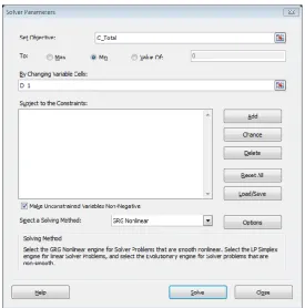
The diameter that minimises the total cost can be found by using the Solver add-in, which is an iterative “What-if analysis” tool developed by Frontline Systems [9]. Found in the “Data” tab, Solver can be used to find the maximum or minimum value of the function in a “target cell”. Solver can adjust the values of a group of cells - called the “adjustable cells” - that are related either directly or indirectly to the formula in the target cell- to produce a specified value for the formula in the target cell. Fig. 3 shows the dialog box for Solver set-up for finding the value of D1 (in the adjustable cell) that minimises the total cost (in the target cell).Fig. 4 shows the sheet with the solution found by Solver. Excel’s solution, which is 0.045763 m, agrees well with the value given by Janna [1].
Vol. 5, Issue 1, January 2016
Fig. 4. Optimised solution for insulated pipe
One of the advantages of computer-aided optimisation compared to analytical optimisation,which is illustrated by this example, is that itinvolves the basic equations without differentiation. However, the really significant advantage of the computer-aided procedure is realised when the optimisation process involves multiple parameters and not just a single parameter likeD1 in this example.We can also apply constraints on the solution which refer to other cells that affect the formula in the target cell directly or indirectly. As the following example demonstrates, thecomputer-aided method can also be applied even whenthe mathematical model is more elaborate and involves lengthy calculationsthat make the optimisation problems impossible to solve analytically.
III.OPTIMISATION OF AN INSULATED AIR-CONDITIONING DUCT
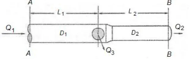
Heated air enters the 30-m air-handling duct shown in Fig.5 at P1 = 100 kPa and T1 =80oC. The flow rate at the entrance is Q1 = 0.7 m3/s, part of whichis discharged at a point 16 m downstream of the duct entrance(Q3=0.3 m3/s). The remaining part is discharged at the end (Q2 = 0.4 m3/s). The air duct is to be assembled from 1-m-long prefabricated units made of galvanized sheet metal and, in order to minimise heat losses to the surroundings, it is desired to insulate the duct. Determine the diameters of the two duct sections (D1 and D2) and the thickness of insulation on both sections (ts,1 and ts,2) that minimise the total owning cost based on the data provided below.
Fig. 5. The uninsulated air-conditioning duct
Air data:
Ambient temperature (T∞2) = 15oC
Outside heat-transfer coefficient h2 = 30 W/m2. oC
Duct data:
Length of first section(L1) = 14 m
Thermal conductivity (kd) = 18 W/m.oC Roughness height (ε) = 0.045mm
Cost of 1-m unit (cd) is as shown in Table 1
Insulation data: Type: fiberglass
Thermal conductivity (ks) = 0.04 W/m.oC Insulation cost (cs1): 30 $/m2 per cm of insulation Labour cost (cs2): 10 $/m2 (irrespective of thickness)
Table 1. Unit cost of the duct body [10] Diameter Cost per 1 m
(Di) in m length ($)
0.1 9
0.15 11.5 0.2 14.5 0.25 17 0.3 22.5 0.35 29
0.4 34
0.45 40
0.5 50
Operation data:
365 days per year 24 hours per day
Energy costs:
Cost of electricity (cE): 0.12 $/kWh
Cost of fuel (cF): 0.5 $/therm (1 therm = 105500 kJ)
Capital recovery factor (i) = 0.15
IV.THE ANALYTICAL MODEL
The total annual costof the insulated air-duct (CTotal) consists of three components asexpressed by:
F E I
Total C i C C
C ($) (6)
Where:
CI = initial cost which consists of the cost of the duct itself plus the cost of insulation
i
= capital recovery factorCE = cost of electricity consumed by the fan in order to overcome friction in the duct CF = cost of fuel needed to make-up for the heat loss to the surrounding air
The analytical model describes how the three components of the total cost are evaluated.
a) Initial cost
The initial cost (CI) has two parts: (1) the cost of the duct itself (Cduct) and (2) the cost of insulation (Cins). The two parts are given by:
Cduct =
D1cd,1
L1
D2cd,2
L2 (7) Cins =
D1L1
ts,1
D2L2
ts,2
cs1
D1L1
D2L2
cs2 (8)Where:
d
c = cost of 1-m duct unitwhich depends on the diameter ($/m)
1 , s
c
= cost of insulation per m2 that varies with insulation thickness ($/m2.cm)2 , s
c
= cost of labour per m2 that depends on insulated surface area only ($/m2)Vol. 5, Issue 1, January 2016 ) . / ($ ) ( )
(kW timehr c kWhr W
CE fan E ($) (9)
Where, Wfanis the power consumed by the air-circulation fan and cE is the electricity tariff in $/kW.hr. The power of the circulation fan depends on the friction head losses (hL)in both sections of the duct which are given by the Darcy-Weisbach equation [11]:
g V D L f hL 2 2
(m) (10)
Where fis the friction factor in each section of the duct which depends on the Reynolds number in the section and can be obtained from the following equation [11].
2 9 . 0 10 Re 74 . 5 7 . 3 log / 25 . 0 D
f (11)
Where the roughness height (ε) is in m. The total power consumed by the air-circulation fan (Wfan) is then
determined from:
1000 2 2 , 1 1,Q h Q
h g
Wfan
air L L (kW) (12)c) Annual cost of fuel:
F Total F c hr time W Q C 105500 1000 ] [ ] [
($) (13)
Where, cF is the cost of fuel in $/therm. The total heat loss (QTotal) is the sum of the heat loss in both sections, i.e.
Total
Q = Q1+Q2, where the heat loss (Q) in each section is calculated according to the formula:
Total R
T T
Q 1 2 (W) (14)
Where T∞1 and T∞2 are the inside and outside air temperatures and RTotal is the total thermal resistance given by:
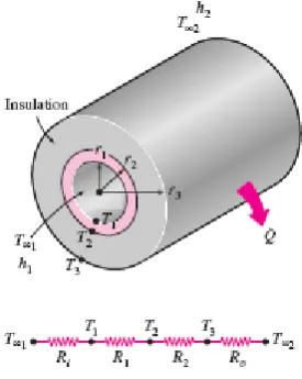
L h r L k r r L k r r L h r R s d Total 2 3 2 3 1 2 1 1 2 1 2 / ln 2 / ln 2 1 (15)The radii r1, r2 and r3 used in Eq. (15) are as shown in Fig. 6. Note that the value of the outside heat-transfer coefficient (h2) is constant, but the inside heat-transfer coefficient (h1),which depends on the air velocity, changes with the
inside diameter of the duct and therefore,has to be determined from the Nusselt number (Nu):
Nu D k
h air
1
For fully developed turbulent flow in smooth tubes, the Nusselt number is calculated from the Dittus– Boelterequation [12]:
3 . 0 8 . 0
Pr Re 023 .
0 i
Nu (17)
Where Re and Pr are the Reynolds and Prandtl numbers, respectively.
Fig. 6. Total thermal resistance of the insulated duct
V. EXCEL MODELAND SOLUTION
The Excel sheet developed for this example uses the relationships described in the previous section to determine the total annual cost for guessed values of the diameters (D1and D2) and insulation thicknesses (ts,1andts,2) in the two sections of the dutc. Solver is then used to find the optimum values of D1, D2, ts,1andts,2. The set-up box for Solver requires it to minimise the total cost (C_total),which is the target cell, by changing the values of the two diameters (D1, D2) and the two insulation thicknesses (ts,1, and ts,2), which are the adjustable cells. To allow Excel to automatically calculate the cost of duct unit (cd) when the two duct diametersare changed, the following equation for cd was obtained from the data shown in Table 1 by using Excel’s trendline:
2 91 . 169 7814 . 1 6881 .
7 D D
cd (18)
Properties of air at 80oC were obtained from Cengel and Ghajar [12]. The optimised dimensions found by Solver are shown in Table 2 which also shows the different cost involved. The nearest dimeters are D1=0.4m and D2=0.3 m. Both insualtion thicknesses are ≈ 0.3 m. The total annual cost sums up to 479.7 $.
Table 2. Solver solution for the insulated duct Values found
without Eq. (19) (m)
Values found with Eq. (19) (m) D1(m) 0.4142 0.4525 D2(m) 0.2951 0.2586
1 , s
t (m) 0.2970 0.2953
2 , s
t (m) 0.3023 0.3056
Cduct($) 128.5113 132.1191 Cins($) 95.7092 95.2828 CE ($) 182.7827 186.4329 CF ($) 72.6776 72.3330 CTotal($) 479.6808 486.1678
Vol. 5, Issue 1, January 2016
1 1 3
2 Q /Q D
D (19)
Let us now determine the optimum diameters and insulation thicknesses by applying Eq. (19). SinceD2 is related to D1 by Eq. (19), it cannot be used as an adjustable cell. The solution determined by Solver with D1, ts1 and ts2 as adjustable cellsis also shown in Table 2.Compared to the solution obtained without Eq. (19),the rule-of-thump leads to a larger D1and a smaller D2. Although the insulation thicknesses on the two section are only marginaly affected, the figures in the table show that the total cost (486.2$) has increased due to increases in the initial cost of the duct (132.1$) as well as the annual cost of electricity (186.4$).
By suitably adjusting the given data, the Excel sheet can be used to study the effects of electricity cost, fuel cost, or capital recovery factor on the opimised solution.With minor modifications the sheet can also be used to optimise a duct carrying cooled air instead of heated air. In this case, the fuel cost (CF) in Eq. (6) should be replaced by the cost of electricity consumed by the refrigeration system (CE2) which can be calculated from:
E Total
E c
COP hr time W Q
C
1000
] [ ] [ 2
(20)
Where COP is the coefficient of performance of the refrigeration system. Eq. (17) also has to be modified as follows:
4 . 0 8 . 0 Pr Re 023 .
0 i
i
Nu (21)
VI. CONCLUSIONS
This paper demonstratesthe advantages ofcomputer-aided optimisation compared to analytical optimisation by presenting two examples of thermal systemsthat use Microsoft Excel and its Solver add-in in the optimisation process. The first exampleshows thatcomputer-aided optimisation,which doesn’t require differentiation, is simpler to apply than analytical optimisation. Optimisation of the insulated duct considered in the second example can only be done with computer-aided optimisationsince the analytical modelinvolves multiple parameters. Analyticaloptimisationcannot be used in this example also becauseof the lengthy calculations and empirical equations involved.Moreover, once developed the Excel sheet can be used to study the effect of various design parameters and operating conditions on the design of thermal systems.
REFERENCES
[1] Janna, W.S., Design of Fluid Thermal Systems, 3rd Edition, CENGAGE Learning, 2011.
[2] Cengel, Y.A. and Boles, M.A.,Thermodynamics an Engineering Approach, McGraw-Hill, 7th Edition, 2007
[3] Moran,M.J. and Shapiro,H.N.. Fundamentals of Engineering Thermodynamics, 5th edition, John Wiley & Sons Inc. 2006.
[4] El-Awad, M.M., Thermax: A Multi-Subject Excel Add-in for Thermal-Fluid Analyses. DOI: 10.13140/RG.2.1.5178.2482 Available online at ResearchGate: https://www.researchgate.net/profile/Mohamed_El-Awad,2015.
[5] Holman,J.P. , Heat Transfer, 10th edition, McGraw Hill, 2010.
[6] Schumack,M., “Use of a Spreadsheet Package to Demonstrate Fundamentals of Computational Fluid Dynamics and Heat Transfer”, Int. J. Engng Ed. Vol. 20, No. 6, pp. 974-983, 2004.
[7] Karimi,A., “A compilation of Examples for using Excel in Solving heat transfer problems”, presented at 2009 Annual Conference & Exposition of the American Society for Engineering Education (ASE), 2009, Austin Texas.
[8] Karimi,A., “Using Excel for the thermodynamic analyses of air-standard cycles and combustion processes”, ASME 2009 Lake Buena Vista, Florida, USA.
[9] Frontline Systems, internet: http://www.Solver.com/(Last accessed November 23, 2015).
[10] The duct shop, https://www.theductshop.com/shop/catalog-galvanized-sheet-metal-duct-c-1_3.html, last accessed 24/12/2015. [11] Crowe,C. T., Elger,D. F., Wiliams , B. C., and Roberson,J. A., Engineering Fluid Mechanics, 9th edition, 2009.
![Table 1. Unit cost of the duct body [10] Diameter](https://thumb-us.123doks.com/thumbv2/123dok_us/1654912.1207441/5.595.355.489.189.318/table-unit-cost-duct-body-diameter.webp)